The Coverage of Elliptical Orbits Using Ergodic Theory Martin W. Lo Jet Propulsion Laboratory California Institute of Technology 4800 Oak Grove Dr., MS 301/140L Pasadena, CA 9 1 109 8 18-354-7169
[email protected]
Abstract-One of the key performance metrics for satellite constellations is the statistics of the visibility periods between the satellites and points on the ground. Associated with this are other desirable communications statistics such as data through-put, link qualities, etc. Typically, the computation of coverage statistics requires the propagation of the trajectories. For orbits with non-repeating ground tracks, this may require orbit propagation for tens of years per spacecraft. Lo [ 11 proposed an approach using ergodic theory which replaced the need to compute the statistics from integrated trajectories by a definite integral over the circular region of the elevation mask of a point on the ground. The effects of J2 due to the non-spherical shape of the Earth are included in the definite integral. The definite integral can be implemented in Excel for quick trade studies. But the simple geometric methods used to derive the integral for circular orbits cannot be readily extended to elliptical orbits. In this paper a new algorithm using differential geometry enables us to extend this theory to elliptical orbits.
Network on Earth through a telecommunications spacecraft orbiting Mars, such as the Mars Telecommunications Orbiter. Lo [ 11 and [2] proposed the use of ergodic theory to compute satellite coverage performance. This simplified the computation of quantities such as the total time for which a ground station can see a satellite without integrating the trajectory. More over, for any quantity which is an integrable function of the satellite position or ground track, its average may be computed similarly without the integration of the trajectory. For example, the data rate for a simple telecom system is a function of the distance between the satellite and the ground station (see Lo [3]). However, these results required that the satellite orbits be circular. In this paper, we extend these results, theoretically, to elliptical orbits using a new approach with differential geometry. The numerical implementation of this approach will be treated in subsequent papers. The Coverage Analysis Problem, at its simplest, is the study of the visibility properties of a satellite in orbit around the Earth from a point on Earth. In Figure 1, we depict the satellite ground track of a circular inclined orbit and the circular region of visibility from a point P (at the center of the circle) on the Equator in the Pacific Ocean. Geometrically, whenever the satellite ground track enters this circle, it is in view from the station on the Equator. We define the following variables for this discussion. Let D be the circular region of visibility of a spacecraft from a ground station centered on the Equator in the Pacific Ocean. Let A be the annulus region defined by the ground tracks of the spacecraft. Let x(D) denote the area function, in this example, the area of the region D on the sphere (the Earth). See Figure 1.
TABLE OF CONTENTS
.....................................................................
1. INTRODUCTION.............................^ 2. ERGODIC THEORY..................... 2 3. CIRCULAR ORBIT CASE... 3 4. ELLIPTICAL ORBIT CASE. .4
..... ................ ............... 5. CONCLUSIONS AND FUTURE WORK.... 4 REFERENCES....... ........................... 5 APPENDIX.. ..................................... 6 1. INTRODUCTION
The Satellite Coverage Analysis Problem is the study of the statistics of interactions between a satellite and other objects in space. The most common example of this problem is the analysis of the visibility of satellites to ground stations on Earth. A more complex problem is the analysis of the coverage between a rover on Mars and the Deep Space
Simplistically, one may think that the percentage of time T spent by the satellite in the circle D would be well approximated by the area of the intersection between the circle and the annulus defined by the ground track, divided by the area of the annulus defined by the ground track, Le., T would be equal to the expression: N ( A n D ) 1 x ( A ) .
' 0-7803-8155-6/04/$17.0082004 IEEE
'IEEEAC paper #l466, Version 3, UpdatedDecember 10,2003 1
In fact, this is a very bad approximation. A clue as to why this is a bad approximation is given by the density of the ground tracks which depends on the latitude and is quite uneven. Moreover, the speed of the nadir of the satellite along the ground track is not constant because the Earth is rotating. Also, the orbital plane is precessing due to the J2 gravity harmonic. But all is not lost.
equations, whereas space average is much easier to compute as it requires only a single area integral. Note, for the space average, J2 is only used for the verification that the orbit ground track is not periodic, it never enters into the area integral. We should note here that we are assuming that the satellite orbit is being maintained so that effects of the Earth gravity’s higher harmonics, the luni-solar perturbation, solar radiation pressure, and drag are being compensated. The maneuvers will perturb the orbit node, but the orbital elements such as semimajor axis and eccentricity are essentially preserved. Assuming the maneuvers are sufficiently random without a bias that would cause the ground tracks to become periodic in some fashion, then this theory applies to the coverage problem.
The heuristics of this reasoning is intuitively correct. But, instead of the ratio of the geometric areas of the two regions mentioned earlier, we need to weigh the area depending on the ground velocity and some how account for the expansion and contraction of the ground tracks. This new weighted area function is technically called an “invariant measure” usually denoted by “p.” Measure is a generalization of the concept of area and volume for sets of arbitrary dimensions. As a weighted area element (an infinitesimal piece of the sphere) following the satellite nadir along the ground track, the area of the element is preserved. Hence the weighted area element is invariant under the motion of the satellite ground track. When such a measure of the area is available, then indeed the percentage of time spent by the satellite in the circular region is given by the measure of the intersection of the circular region with the annulus, divided by the measure of the annulus, i.e., T is equal to the expression: p ( A nD ) / p ( A ).
2. ERGODIC THEORY Ergodic theory has its origins in the study of statistical mechanics in the 19” century. Maxwell, Boltzmann, Gibbs, and PoincarC were the first to propose a statistical approach to study differential equations. A classical problem is the following: Given a particle moving randomly within a closed and bounded box B; at time 0 the particle is known to be in the subset C of our box B; how frequently will this particle visit the subset C within our box as the time goes to infinity? PoicarC’s Recurrence Theorem tells us that the particle will repeatedly visit the set C infinitely often (see Sinai [4] and [5].In fact, the probability that the particle can be found in C is given by the volume of the set C divided by the volume of the box B. This is geometrically intuitive.
Such a measure was constructed in Lo [ 11 and [2]. However, for this to work, it is necessary that the ground tracks not be periodic. But it is shown that even when the ground track is periodic, provided the repeat cycle is not too small, this approximation is fairly good. This methodology means that instead of finding the view periods from a propagated trajectory to compute the amount of time a satellite is in view of a ground station, also called the “time average”, we can replace this by a simple area integral with a weighted area. This weighted average is called the “space average.” This method in essence is an application of the Ergodic Theorem that we can replace time averages by space average. Typically, time average is more difficult to compute since it requires the solution of differential
/
An‘\
& -
’
\
The fact that the probability the particle can be found in the set C is given by the quantity Volume( C ) / Volume ( B ) is a profound result. Our original question is about the time average of the particle visiting the set C; our answer is that it is given by the space average of the set C, Le., its volume normalized by the total volume of the box B. This equivalence of “time average” with “space average” is at the heart of ergodic theory. The reason this is so powerful is because we can replace knowledge of the time history of a particle (its trajectory) in a dynamical system (a set of differential equations) by a definite integral over subsets within the phase space (such as the 6-dimensional state space of position and velocity for a satellite). In other words, without integrating the differential equations, we can obtain valuable statistical information about the dynamical systems by computing definite integrals which are often much easier to do.
\
In order to apply ergodic theory to a dynamical system described by a set of differential equations, one must first obtain a volume function on the phase space which is invariant under the trajectory flow cp,(x) prescribed by the differential equations. The flow cp t(x) is the solution to the differential equation at time “t” with initial condition “x” in
:/ \ -
Figure 1. The ground tracks of a satellite in circular orbit forming the annulus A and the circular coverage region D of a fictitious station P in the Pacific on the Equator. 2
the phase space. It describes the complete set of solutions to the differential equation. The analogy is to streamlines in a fluid flow. This is known as an “invariant measure”; it is just a volume element weighted by a h c t i o n to compensate for the contractions and expansions of the trajectories in the phase space. In our case, the trajectory flow is the ground tracks of the satellite and the phase space is replaced by the spherical surface of the planet. The measure is ordinary spherical area multiplied by a weighting function. The construction of the invariant measure is the hard part of the problem. For our problem, this has been done in Lo [l]. We denote this measure, or the volume function by p, which is normalized to give a total volume equal to 1. We indicate the differential volume element by dp. We now define more precisely what we mean by time and space averages.
The expression for the invariant measure itself, dp, does not include the Jz coefficient. The long-term station view period ratio p is defined by Lo [ 11 as p
M , t e R.
lim -p,m
T+-
T
(3)
where P(T) is the total time the satellite is in view of the ground station from time 0 to time T. In other words, p is the fraction of time the satellite can see the ground station; and pT gives a good approximation for value of P(T) for sufficiently large T. In this case, the function f (x) is the characteristic function of the station mask, D (e.g. see Figures 1 and 2). In other words, f (x) is 1 when x is in D and 0 otherwise. The set D is the circular region on the planet centered around the ground station defined by the minimum elevation angle E of the ground station. For details see Lo [ 11.
The time average < f > of a function f is defined by:
XE
=
Figure 3 shows the power of this approach. We are able to provide the global coverage properties of all circular orbits at 3900 km altitude to every point on the Earth using the visibility ratio, p. computed from the space average integral. This required a few seconds to compute. Whereas if we were to compute this using the integration of trajectories, it would require many hours, perhaps even days of computation to provide such a result. The simplicity of the equations allows analysts to use them in tools such as Excel or Mathematica for quick studies of coverage analysis. At 90” and critical inclinations, the result still holds even though the nodal regression due to J2 is absent, the rotation of the planet continues to spread the satellite ground track around the planet where ergodicity of the ground tracks is possible. However, the condition for the commensurability of the orbital period with the rotation of the ground tracks will no longer include the J2 term which is 0 for these cases.
-
The space average of a function f is defined by:
Here x is a point in the phase space M, and R is the set of real numbers. The fundamental theorem of ergodic theory is the Birkhoff-Khinchin theorem (Theorem 6.4 in Amold [ 6 ] ) which simply states that the time mean (1) is equal to the space mean (2) for ergodic dynamical systems. In other
-
words, that < f > is equal to f . We will not get into the details of the necessary conditions for this theorem to hold; suffice it to say that for satellite motion under the gravitation of an oblate planet, these conditions are satisfied.
3. CIRCULAR ORBIT CASE We first review the results from Lo [l] for the view period problem. Given a ground station located at “x” on Earth, we want the amount of time the ground station is in view of the satellite. We assume the satellite is moving in a circular orbit about an oblate planet with Jz perturbation resulting in the drifting of the ascending node of the orbit. However, to compute the station visibility, we treat the planet as a sphere. In order for the Birkhoff-Khinchin Theorem to apply, we must further assume that the orbital ground track is not repeating. Although this excludes some of the most important satellite orbits, all is not lost. For those orbits with short ground track repeat cycles, the statistics may be quickly computed using the standard trajectory integration approach. For those orbits with long repeat cycles, the ergodic theory provides a reasonable approximation for quick analyses as noted in Lo [l]. The interesting thing is that the only place where the value of 52 is needed is in the verification that the satellite ground track is non-repeating.
Figure 2. Definition and geometry of the visibility mask and angles for a station at the top of the Earth to a spacecraft (SIC). 3
trajectories generated by E as a fluid flow, the fluid is incompressible. So the problem is reduced to finding a new volume, s, in which div(z) is 0, where Z is the vector field associated with our flow or the sky-track, d t ) . This approach allowed us to find a partial differential equation which fortunately reduces to an ordinary differential equation for the volume, s. The derivation and the equations are shown in the Appendix. To obtain the invariant measure, we need the equations for the flow d t ) . For this we can use the linear approximation for the regression of the node and the argument of periapsis caused by J2. We then transform it into the Earth-fixed coordinate system to produce d x ) . One other technical point is that we need to treat the ascending and descending trajectories separately in order for the trajectories in the flow not to intersect one another. This issue is discussed for the circular orbit case in Lo [ 11.
Figure 3. The total visibility for any satellite at 3900 km altitude to every point on the Earth. The X-axis is orbital inclination, the Y-axis is station latitude, and the Z-axis is the total visibility period in minutes per day.
5. CONCLUSIONS AND FUTURE WORK These results, such as in Figure 3, have been compared with conventional view period computations using propagated satellite trajectories. The difference between the view period predicted by the ergodic theory and by the conventional method is less than 1%. For orbits with repeat ground tracks of larger periods (around 10 days), the accuracy is less than 2%. But, for elliptical orbits even with e=0.05, the errors can be more than 16%, see Lo [ 11. A new formulation is needed for elliptical orbits.
In this paper we extended the theory for computing the longterm station view period ratio, p, of circular orbits to ellipcital orbits without integrating the trajectory. The fundamental idea is to change the volume where the trajectory moves to provide a new volume which is invariant under the flow the trajectories. This then allows one to apply the Ergodic Theorem. In the case of circular orbits, elementary geometric methods enabled one to solve this problem. For elliptical orbits, this is much more difficult. By implementing the idea using differential geometry we were able to construct a new volume function as detailed in the Appendix.
4. ELLIPTICAL ORBIT CASE For the circular orbit case, it is convenient to work with the ground tracks of the spacecraft. However, for elliptical orbits, this becomes a problem because of the extra dimension introduced by the variation in the altitude and the motion of the periapsis. Hence, we no longer look at the ground track. Instead we look at the orbital tracks in 3space as viewed from the earth. In other words, we go into the earth-fured rotating frame and consider the orbit from that perspective. We call this the sky-tracks. For circular orbits, this will reduce to ground tracks. Given a ground station, G, we can draw the cone of visibility over G, call it C(G). Let d t ) denote the sky tracks of the satellite. What we want to know is how often is p(t) in the region C(G). If the tracks d t ) were evenly distributed over C(G), ergodic theory can be applied immediately. But, just like the circular case, the tracks are not evenly distributed. Thus the solution is that we must distort the volume to compensate for the unevenness so that the tracks become evenly distributed. In other words, we need to find a measure or volume which is invariant under the flow of dt). See the Appendix for a more geometric explanation of this concept.
Numerical implementation of the algorithm remains to be completed. Another exercise would be to use this new formulation to derive again the ergodic coverage integral for the circular orbit case. By general ergodic theory, this new integral for elliptical orbital periods can be used to compute the average of many other functions which depend on the orbit. An example is the data throughput of telecommunications systems on the satellite which depends on the orbital parameters.
ACKNOWLEDGEMENTS This work was carried out at the Jet Propulsion Laboratory of the California Institute of Technology under a contract with the National Aeronautics and Space Administration.
REFERENCES
[l] Lo, M.W., “The Long-Term F o y a r 6 6 S t a t i o n View Period”, JPL TDA Progress R e y t . 4 2 - 1 1 8 , pp. 1-14, AprilJune, 1994.
Going back to vector calculus, recall that if the divergence of a vector field, Z, is 0, then volume is conserved by the flow of the vector field. In other words, if we think of the
[2] Lo, M.W., “The Invariant Measure for the Satellite 4
REFERENCES [l] Lo, M.W., “The Long-Term Forecase of Station View Period”, JPL TDA Progress Report 42-118, pp. 1-14, AprilJune, 1994. [2] Lo, M.W.,“The Invariant Measure for the Satellite Ground Station View Period Problem,” C. Simo (ed.),
Hamiltonian Systems with Three or More Degrees of Freedom, NATO AS1 Series, Kluwer Academic Publishers, 1999. [3] Lo, M.W., “Application of Ergodic Theory to Coverage Analysis”, AAS/AIAA Astrodynamics Specialist Conference, AAS03-638, August 3-7,2003,. [4] Sinai, Ya.G., Introduction to Ergodic Theory, Princeton University Press, Princeton, N.J., 1976. [ 5 ] Sinai, Ya.G., Topics in Ergodic Theory, Princeton University Press, Princeton, N.J., 1994. I I
i
[6] Arnold, V.I., A. Avez, Ergodic Problems of Classical Mechanics, Addison Wesley, 1989, New York. [7] Hicks, N., Notes on Differential Geometry, Van Nostrand, New York, 1965.
I I
BIOGRAPHY Martin W. Lo is a mission designer at JPL in the -
Navigation and Mission Design Section and a visiting faculty in the Caltech Computer Science Department. He is Mars currently supporting the Telecommunications Orbiter mission, analyzing the coverage of various orbital options. Lo is a graduate of Caltech with a PhD from Cornell. His profession interests are on mission design and the development of new approaches based on mathematical methods to extend this technology.
5
volume form s. Thus, the problem becomes finding a volume form s under which the divergence of E is 0. The volume form s will be specified by some positive function f:
APPENDIX In this section, using differential geometry, we show that given a vector field E on {R", u}, there exists a volume function, s, on R" which is invariant under the action of E. In other words, the new volume, s, is conserved under the flow of Z. The volume function is frequently referred to as the volume form, since the volume differential, dx dy dz, is a differential form. For references on differential geometry, see Hicks [7]. For our problem, the vector field E is the orbital tracks of the spacecraft in 3-dimensional space, i.e., R3, and "u" is the standard volume on 3-space. The orbital tracks create a flow in R3; in other words they provide the paths for imaginary particles moving in space as if for a fluid. Using the standard volume function denoted by 't", a volume element containing a small group of these particles will expand and contract as they move along the satellite tracks in 3-space. The new volume function "s" will average these expansions and contractions to provide a constant volume for any group of particles flowing along the satellite tracks in 3-space. This is the geometric meaning that the volume function, s, is "conserved under the flow".
s(x) = f(x) u(x)
This reduces the problem to finding the function Qx) which is specified by the following first order PDE: div( f u, E) = div(u, E)+ LE (f)/f = 0
(6)
Let g = In(f), well defined since f > 0, we have Lz(f)/f equal to LE(g), thus (6) becomes: LE (g) = - div(u, E)
(7)
In coordinate form: Ei aig = - div(u, E)
(8)
where Zi is the i" component of E, dig is the partial of of with the ithcoordinate xi. As this is a first order PDE, from the theory of characteristics, it is solved by the following ODE: dddt = - div(u, E( cp(t))) (9)
Assumptions and Notation:
1. All objects are smooth. 2. Let {R", u} be our manifold of dimension n with volume form u. In our case, n = 3 and u = dx dy dz (i.e., dx A dy A dz, in differential form notation). 3. Let Z be our vector field with flow cp(x,t) or At). The flow is the trajectory starting at x at time 0 which has tagent vectors given by Z, i.e. cp'(x, t) = E( q(x, t) ) whee the derivative is with respect to "t" only. 4. LE (f u): Lie derivative of fcu in the direction of E, this is the directional derivative of fcu along the flow of Z. 5. div(u, Z) : divergence of the vector E under the volume form, u. Divergence is a real valued function defined with respect to a metric which in this case is given by the volume form, u. 6. dig : partial derivative of g with i* coordinate, xi. 7. R": Real vector space of dimension n which is 3 here.
which is readily integrated numerically, thereby yielding g: g( cp(t)) = z(t)
(10)
and Qx) is just exp(g(x)). This gives the desired volume form.
Given a vector field E on {W",u}, there exists a volume form, s, on M which is invariant under the action of Z. In other words, volume is conserved under the flow of 2. Using basic differential geometry, we can show this to be true. For references on differential geometric identifies and notations, see Hicks [71. The action of Z on a volume form, s, is completely specified by the Lie derivative of s. For s to be invariant under E is the same as: LE (s) = div(s, E) s = 0 .
(5)
(4)
(4) is just the definition of divergence for a manifold with
6