The Data Compression Book. By Mark Nelson and Jean-loup Gailly. Chapter 1.
Introduction to Data Compression. The primary purpose of this book is to explain
...
CSA215: Data Compression Techniques Course Coordinator: Mr. Basel Bani-Ismail
University of Bahrain College of Applied Studies
The Data Compression Book By Mark Nelson and Jean-loup Gailly
Chapter 1 Introduction to Data Compression The primary purpose of this book is to explain various data-compression techniques. Data compression seeks to reduce the number of bits used to store or transmit information. It encompasses a wide variety of software and hardware compression techniques which can be so unlike one another that they have little in common except that they compress data. The LZW algorithm used in the Compuserve GIF specification, for example, has virtually nothing in common with the CCITT G.721 specification used to compress digitized voice over phone lines. This book will not take a comprehensive look at every variety of data compression. The field has grown in the last 25 years to a point where this is simply not possible. What this book will cover are the various types of data compression commonly used on personal and midsized computers, including compression of binary programs, data, sound, and graphics. Furthermore, this book will either ignore or only lightly cover data-compression techniques that rely on hardware for practical use or that require hardware applications. Many of today’s voice-compression schemes were designed for the worldwide fixed bandwidth digital telecommunications networks. These compression schemes are intellectually interesting, but they require a specific type of hardware tuned to the fixed bandwidth of the communications channel. Different algorithms that don’t have to meet this requirement are used to compress digitized voice on a PC, and these algorithms generally offer better performance. Some of the most interesting areas in data compression today, however, do concern compression techniques just becoming possible with new and more powerful hardware. Lossy image compression, like that used in multimedia systems, for example, can now be implemented on standard desktop platforms. This book will cover practical ways to both experiment with and implement some of the algorithms used in these techniques.
1
CSA215: Data Compression Techniques Course Coordinator: Mr. Basel Bani-Ismail
University of Bahrain College of Applied Studies
Chapter 2 The Data-Compression Lexicon, with a History Like any other scientific or engineering discipline, data compression has a vocabulary that at first seem overwhelmingly strange to an outsider. Terms like Lempel-Ziv compression, arithmetic coding, and statistical modeling get tossed around with reckless abandon. While the list of buzzwords is long enough to merit a glossary, mastering them is not as daunting a project as it may first seem. With a bit of study and a few notes, any programmer should hold his or her own at a cocktail-party argument over data compression techniques.
The Two Kingdoms Data-compression techniques can be divided into two major families; lossy and lossless. Lossy data compression concedes a certain loss of accuracy in exchange for greatly increased compression. Lossy compression proves effective when applied to graphics images and digitized voice. By their very nature, these digitized representations of analog phenomena are not perfect to begin with, so the idea of output and input not matching exactly is a little more acceptable. Most lossy compression techniques can be adjusted to different quality levels, gaining higher accuracy in exchange for less effective compression. Until recently, lossy compression has been primarily implemented using dedicated hardware. In the past few years, powerful lossy-compression programs have been moved to desktop CPUs, but even so the field is still dominated by hardware implementations. Lossless compression consists of those techniques guaranteed to generate an exact duplicate of the input data stream after a compress/expand cycle. This is the type of compression used when storing database records, spreadsheets, or word processing files. In these applications, the loss of even a single bit could be catastrophic. Most techniques discussed in this book will be lossless.
Data Compression = Modeling + Coding In general, data compression consists of taking a stream of symbols and transforming them into codes. If the compression is effective, the resulting stream of codes will be smaller than the original symbols. The decision to output a certain code for a certain symbol or set of symbols is based on a model. The model is simply a collection of data and rules used to process input symbols and determine which code(s) to output. A program uses the model to accurately define the probabilities for each symbol and the coder to produce an appropriate code based on those probabilities.
2
CSA215: Data Compression Techniques Course Coordinator: Mr. Basel Bani-Ismail
University of Bahrain College of Applied Studies
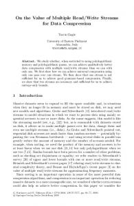
Modeling and coding are two distinctly different things. People frequently use the term coding to refer to the entire data-compression process instead of just a single component of that process. You will hear the phrases “Huffman coding” or “Run-Length Encoding,” for example, to describe a data-compression technique, when in fact they are just coding methods used in conjunction with a model to compress data. Using the example of Huffman coding, a breakdown of the compression process looks something like this:
Figure 2.1 A Statistical Model with a Huffman Encoder. In the case of Huffman coding, the actual output of the encoder is determined by a set of probabilities. When using this type of coding, a symbol that has a very high probability of occurrence generates a code with very few bits. A symbol with a low probability generates a code with a larger number of bits. We think of the model and the program’s coding process as different because of the countless ways to model data, all of which can use the same coding process to produce their output. A simple program using Huffman coding, for example, would use a model that gave the raw probability of each symbol occurring anywhere in the input stream. A more sophisticated program might calculate the probability based on the last 10 symbols in the input stream. Even though both programs use Huffman coding to produce their output, their compression ratios would probably be radically different. So when the topic of coding methods comes up at your next cocktail party, be alert for statements like “Huffman coding in general doesn’t produce very good compression ratios.” This would be your perfect opportunity to respond with “That’s like saying Converse sneakers don’t go very fast. I always thought the leg power of the runner had a lot to do with it.” If the conversation has already dropped to the point where you are discussing data compression, this might even go over as a real demonstration of wit.
The Dawn Age Data compression is perhaps the fundamental expression of Information Theory. Information Theory is a branch of mathematics that had its genesis in the late 1940s with the work of Claude Shannon at Bell Labs. It concerns itself with various questions about information, including different ways of storing and communicating messages.
3
CSA215: Data Compression Techniques Course Coordinator: Mr. Basel Bani-Ismail
University of Bahrain College of Applied Studies
Data compression enters into the field of Information Theory because of its concern with redundancy. Redundant information in a message takes extra bit to encode, and if we can get rid of that extra information, we will have reduced the size of the message. Information Theory uses the term entropy as a measure of how much information is encoded in a message. The word entropy was borrowed from thermodynamics, and it has a similar meaning. The higher the entropy of a message, the more information it contains. The entropy of a symbol is defined as the negative logarithm of its probability. To determine the information content of a message in bits, we express the entropy using the base 2 logarithm: Number of bits = - Log base 2 (probability) The entropy of an entire message is simply the sum of the entropy of all individual symbols. Entropy fits with data compression in its determination of how many bits of information are actually present in a message. If the probability of the character ‘e’ appearing in this manuscript is 1/16, for example, the information content of the character is 4 bits. So the character string “eeeee” has a total content of 20 bits. If we are using standard 8-bit ASCII characters to encode this message, we are actually using 40 bits. The difference between the 20 bits of entropy and the 40 bits used to encode the message is where the potential for data compression arises. One important fact to note about entropy is that, unlike the thermodynamic measure of entropy, we can use no absolute number for the information content of a given message. The problem is that when we calculate entropy, we use a number that gives us the probability of a given symbol. The probability figure we use is actually the probability for a given model, not an absolute number. If we change the model, the probability will change with it. How probabilities change can be seen clearly when using different orders with a statistical model. A statistical model tracks the probability of a symbol based on what symbols appeared previously in the input stream. The order of the model determines how many previous symbols are taken into account. An order-0 model, for example, won’t look at previous characters. An order-1 model looks at the one previous character, and so on. The different order models can yield drastically different probabilities for a character. The letter ‘u’ under an order-0 model, for example, may have only a 1 percent probability of occurrence. But under an order-1 model, if the previous character was ‘q,’ the ‘u’ may have a 95 percent probability. This seemingly unstable notion of a character’s probability proves troublesome for many people. They prefer that a character have a fixed “true” probability that told what the chances of its “really” occurring are. Claude Shannon attempted to determine the true information content of the English language with a “party game” experiment. He would 4
CSA215: Data Compression Techniques Course Coordinator: Mr. Basel Bani-Ismail
University of Bahrain College of Applied Studies
uncover a message concealed from his audience a single character at a time. The audience guessed what the next character would be, one guess at a time, until they got it right. Shannon could then determine the entropy of the message as a whole by taking the logarithm of the guess count. Other researchers have done more experiments using similar techniques. While these experiments are useful, they don’t circumvent the notion that a symbol’s probability depends on the model. The difference with these experiments is that the model is the one kept inside the human brain. This may be one of the best models available, but it is still a model, not an absolute truth. In order to compress data well, we need to select models that predict symbols with high probabilities. A symbol that has a high probability has a low information content and will need fewer bits to encode. Once the model is producing high probabilities, the next step is to encode the symbols using an appropriate number of bits.
Coding Once Information Theory had advanced to where the number of bits of information in a symbol could be determined, the next step was to develop new methods for encoding information. To compress data, we need to encode symbols with exactly the number of bits of information the symbol contains. If the character ‘e’ only gives us four bits of information, then it should be coded with exactly four bits. If ‘x’ contains twelve bits, it should be coded with twelve bits. By encoding characters using EBCDIC or ASCII, we clearly aren’t going to be very close to an optimum method. Since every character is encoded using the same number of bits, we introduce lots of error in both directions, with most of the codes in a message being too long and some being too short. Solving this coding problem in a reasonable manner was one of the first problems tackled by practitioners of Information Theory. Two approaches that worked well were Shannon- Fano coding and Huffman coding—two different ways of generating variable-length codes when given a probability table for a given set of symbols. Huffman coding, named for its inventor D.A. Huffman, achieves the minimum amount of redundancy possible in a fixed set of variable-length codes. This doesn’t mean that Huffman coding is an optimal coding method. It means that it provides the best approximation for coding symbols when using fixed-width codes. The problem with Huffman or Shannon-Fano coding is that they use an integral number of bits in each code. If the entropy of a given character is 2.5 bits, the Huffman code for that character must be either 2 or 3 bits, not 2.5. Because of this, Huffman coding can’t be considered an optimal coding method, but it is the best approximation that uses fixed codes with an integral number of bits. Here is a sample of Huffman codes:
5
CSA215: Data Compression Techniques Course Coordinator: Mr. Basel Bani-Ismail
University of Bahrain College of Applied Studies
An Improvement Though Huffman coding is inefficient due to using an integral number of bits per code, it is relatively easy to implement and very economical for both coding and decoding. Huffman first published his paper on coding in 1952, and it instantly became the most cited paper in Information Theory. It probably still is. Huffman’s original work spawned numerous minor variations, and it dominated the coding world till the early 1980s. As the cost of CPU cycles went down, new possibilities for more efficient coding techniques emerged. One in particular, arithmetic coding, is a viable successor to Huffman coding. Arithmetic coding is somewhat more complicated in both concept and implementation than standard variable-width codes. It does not produce a single code for each symbol. Instead, it produces a code for an entire message. Each symbol added to the message incrementally modifies the output code. This is an improvement because the net effect of each input symbol on the output code can be a fractional number of bits instead of an integral number. So if the entropy for character ‘e’ is 2.5 bits, it is possible to add exactly 2.5 bits to the output code. An example of why this can be more effective is shown in the following table, the analysis of an imaginary message. In it, Huffman coding would yield a total message length of 89 bits, but arithmetic coding would approach the true information content of the message, or 83.56 bits. The difference in the two messages works out to approximately 6 percent. Here are some sample message probabilities:
6
CSA215: Data Compression Techniques Course Coordinator: Mr. Basel Bani-Ismail
University of Bahrain College of Applied Studies
The problem with Huffman coding in the above message is that it can’t create codes with the exact information content required. In most cases it is a little above or a little below, leading to deviations from the optimum. But arithmetic coding gets to within a fraction of a percent of the actual information content, resulting in more accurate coding. Arithmetic coding requires more CPU power than was available until recently. Even now it will generally suffer from a significant speed disadvantage when compared to older coding methods. But the gains from switching to this method are significant enough to ensure that arithmetic coding will be the coding method of choice when the cost of storing or sending information is high enough.
Modeling If we use an automotive metaphor for data compression, coding would be the wheels, but modeling would be the engine. Regardless of the efficiency of the coder, if it doesn’t have a model feeding it good probabilities, it won’t compress data. Lossless data compression is generally implemented using one of two different types of modeling: statistical or dictionary-based. Statistical modeling reads in and encodes a single symbol at a time using the probability of that character’s appearance. Dictionary based modeling uses a single code to replace strings of symbols. In dictionary-based modeling, the coding problem is reduced in significance, leaving the model supremely important.
Statistical Modeling The simplest forms of statistical modeling use a static table of probabilities. In the earliest days of information theory, the CPU cost of analyzing data and building a Huffman tree was considered significant, so it wasn’t frequently performed. Instead, representative blocks of data were analyzed once, giving a table of character-frequency counts. Huffman encoding/decoding trees were then built and stored. Compression programs had access to this static model and would compress data using it. 7
CSA215: Data Compression Techniques Course Coordinator: Mr. Basel Bani-Ismail
University of Bahrain College of Applied Studies
But using a universal static model has limitations. If an input stream doesn’t match well with the previously accumulated statistics, the compression ratio will be degraded— possibly to the point where the output stream becomes larger than the input stream. The next obvious enhancement is to build a statistics table for every unique input stream. Building a static Huffman table for each file to be compressed has its advantages. The table is uniquely adapted to that particular file, so it should give better compression than a universal table. But there is additional overhead since the table (or the statistics used to build the table) has to be passed to the decoder ahead of the compressed code stream. For an order-0 compression table, the actual statistics used to create the table may take up as little as 256 bytes—not a very large amount of overhead. But trying to achieve better compression through use of a higher order table will make the statistics that need to be passed to the decoder grow at an alarming rate. Just moving to an order 1 model can boost the statistics table from 256 to 65,536 bytes. Though compression ratios will undoubtedly improve when moving to order-1, the overhead of passing the statistics table will probably wipe out any gains. For this reason, compression research in the last 10 years has concentrated on adaptive models. When using an adaptive model, data does not have to be scanned once before coding in order to generate statistics. Instead, the statistics are continually modified as new characters are read in and coded. The general flow of a program using an adaptive model looks something like that shown in Figures 2.2 and 2.3.
Figure 2.2 General Adaptive Compression.
8
CSA215: Data Compression Techniques Course Coordinator: Mr. Basel Bani-Ismail
University of Bahrain College of Applied Studies
Figure 2.3 General Adaptive Decompression. The important point in making this system work is that the box labeled “Update Model” has to work exactly the same way for both the compression and decompression programs. After each character (or group of characters) is read in, it is encoded or decoded. Only after the encoding or decoding is complete can the model be updated to take into account the most recent symbol or group of symbols. One problem with adaptive models is that they start knowing essentially nothing about the data. So when the program first starts, it doesn’t do a very good job of compression. Most adaptive algorithms tend to adjust quickly to the data stream and will begin turning in respectable compression ratios after only a few thousand bytes. Likewise, it doesn’t take long for the compression-ratio curve to flatten out so that reading in more data doesn’t improve the compression ratio. One advantage that adaptive models have over static models is the ability to adapt to local conditions. When compressing executable files, for example, the character of the input data may change drastically as the program file changes from binary program code to binary data. A well-written adaptive program will weight the most recent data higher than old data, so it will modify its statistics to better suit changed data.
Dictionary Schemes Statistical models generally encode a single symbol at a time— reading it in, calculating a probability, then outputting a single code. A dictionary-based compression scheme uses a different concept. It reads in input data and looks for groups of symbols that appear in a dictionary. If a string match is found, a pointer or index into the dictionary can be output instead of the code for the symbol. The longer the match, the better the compression ratio. This method of encoding changes the focus of dictionary compression. Simple coding methods are generally used, and the focus of the program is on the modeling. In LZW compression, for example, simple codes of uniform width are used for all substitutions.
9
CSA215: Data Compression Techniques Course Coordinator: Mr. Basel Bani-Ismail
University of Bahrain College of Applied Studies
A static dictionary is used like the list of references in an academic paper. Through the text of a paper, the author may simply substitute a number that points to a list of references instead of writing out the full title of a referenced work. The dictionary is static because it is built up and transmitted with the text of work—the reader does not have to build it on the fly. The first time I see a number in the text like this—[2]—I know it points to the static dictionary. The problem with a static dictionary is identical to the problem the user of a statistical model faces: The dictionary needs to be transmitted along with the text, resulting in a certain amount of overhead added to the compressed text. An adaptive dictionary scheme helps avoid this problem. Mentally, we are used to a type of adaptive dictionary when performing acronym replacements in technical literature. The standard way to use this adaptive dictionary is to spell out the acronym, then put its abbreviated substitution in parentheses. So the first time I mention the Massachusetts Institute of Technology (MIT), I define both the dictionary string and its substitution. From then on, referring to MIT in the text should automatically invoke a mental substitution.
Ziv and Lempel Until 1980, most general-compression schemes used statistical modeling. But in 1977 and 1978, Jacob Ziv and Abraham Lempel described a pair of compression methods using an adaptive dictionary. These two algorithms sparked a flood of new techniques that used dictionary-based methods to achieve impressive new compression ratios.
LZ77 The first compression algorithm described by Ziv and Lempel is commonly referred to as LZ77. It is relatively simple. The dictionary consists of all the strings in a window into the previously read input stream. A file-compression program, for example, could use a 4K-byte window as a dictionary. While new groups of symbols are being read in, the algorithm looks for matches with strings found in the previous 4K bytes of data already read in. Any matches are encoded as pointers sent to the output stream. LZ77 and its variants make attractive compression algorithms. Maintaining the model is simple; encoding the output is simple; and programs that work very quickly can be written using LZ77. Popular programs such as PKZIP and LHarc use variants of the LZ77 algorithm, and they have proven very popular.
10
CSA215: Data Compression Techniques Course Coordinator: Mr. Basel Bani-Ismail
University of Bahrain College of Applied Studies
LZ78 The LZ78 program takes a different approach to building and maintaining the dictionary. Instead of having a limited-size window into the preceding text, LZ78 builds its dictionary out of all of the previously seen symbols in the input text. But instead of having carte blanche access to all the symbol strings in the preceding text, a dictionary of strings is built a single character at a time. The first time the string “Mark” is seen, for example, the string “Ma” is added to the dictionary. The next time, “Mar” is added. If “Mark” is seen again, it is added to the dictionary. This incremental procedure works very well at isolating frequently used strings and adding them to the table. Unlike LZ77 methods, strings in LZ78 can be extremely long, which allows for high-compression ratios. LZ78 was the first of the two Ziv-Lempel algorithms to achieve popular success, due to the LZW adaptation by Terry Welch, which forms the core of the UNIX compress program.
Lossy Compression Until recently, lossy compression has been primarily performed on special-purpose hardware. The advent of inexpensive Digital Signal Processor (DSP) chips began lossy compression’s move off the circuit board and onto the desktop. CPU prices have now dropped to where it is becoming practical to perform lossy compression on general purpose desktop PCs. Lossy compression is fundamentally different from lossless compression in one respect: it accepts a slight loss of data to facilitate compression. Lossy compression is generally done on analog data stored digitally, with the primary applications being graphics and sound files. This type of compression frequently makes two passes. A first pass over the data performs a high-level, signal-processing function. This frequently consists of transforming the data into the frequency domain, using algorithms similar to the wellknown Fast Fourier Transform (FFT). Once the data has been transformed, it is “smoothed,” rounding off high and low points. Loss of signal occurs here. Finally, the frequency points are compressed using conventional lossless techniques. The smoothing function that operates on the frequency-domain data generally has a “quality factor” built into it that determines just how much smoothing occurs. The more the data is massaged, the greater the signal loss—and more compression will occur. In the small systems world, a tremendous amount of work is being done on graphical image compression, both for still and moving pictures. The International Standards Organization (ISO) and the Consultive Committee for International Telegraph and Telephone (CCITT) have banded together to form two committees: The JointPhotographic Experts Group (JPEG) and the Moving Pictures Expert Group
11
CSA215: Data Compression Techniques Course Coordinator: Mr. Basel Bani-Ismail
University of Bahrain College of Applied Studies
(MPEG). The JPEG committee has published its compression standard, and many vendors are now shipping hardware and software that are JPEG compliant. The MPEG committee completed an intial moving picture compression standard, and is finalizing a second, MPEG-II. The JPEG standard uses the Discrete Cosine Transform (DCT) algorithm to convert a graphics image to the frequency domain. The DCT algorithm has been used for graphics transforms for many years, so efficient implementations are readily available. JPEG specifies a quality factor of 0 to 100, and it lets the compressor determine what factor to select. Using the JPEG algorithm on images can result in dramatic compression ratios. With little or no degradation, compression ratios of 90–95 percent are routine. Accepting minor degradation achieves ratios as high as 98–99 percent. Software implementations of the JPEG and MPEG algorithms are still struggling to achieve real-time performance. Most multimedia development software that uses this type of compression still depends on the use of a coprocessor board to make the compression take place in a reasonable amount of time. We are probably only a few years away from software-only real-time compression capabilities.
12