over the first method whenever one is interested in piecing together several polynomial curves. More detail can be found in Crouch, Silva Leite, and. Run [13].
JOURNAL OF DYNAMICAL AND CONTROL SYSTEMS, Vol. 5, No. 3, 1999, 397-429
THE DE CASTELJAU ALGORITHM ON LIE GROUPS AND SPHERES P. CROUCH, G. KUN, F. SILVA LEITE
ABSTRACT. We examine the De Casteljau algorithm in the context of Riemannian symmetric spaces. This algorithm, whose classical form is used to generate interpolating polynomials in Rn, was also generalized to arbitrary Riemannian manifolds by others. However, the implementation of the generalized algorithm is difficult since detailed structure, such as boundary value expressions, has not been available. Lie groups are the most simple symmetric spaces, and for these spaces we develop expressions for the first and second order derivatives of curves of arbitrary order obtained from the algorithm. As an application of this theory we consider the problem of implementing the generalized De Casteljau algorithm on an m-dimensional sphere. We are able to fully develop the algorithm for cubic splines with Hermite boundary conditions and more general boundary conditions for arbitrary m.
1. INTRODUCTION The problem of synthesizing a smooth motion of a rigid body or groups of rigid bodies, such as robots, that interpolates a set of configurations in space has considerable importance in many engineering applications. Other direct applications include path planning for aerospace vehicles. In this context, Crouch and Jackson [14], [15], and [16], and Jackson [17] developed a concept of dynamic interpolation, in which the usual interpolation concept is generalized to include the case where the interpolating curves are generated by dynamical systems. Such problems turn out to be very much more 1991 Mathematics Subject Classification. 22E15, 53E35. Key words and phrases. De Casteljau algorithm, symmetric spaces, Lie groups, spheres, polynomial curves, cubic splines, covariant derivatives. The first author was supported in part by NATO, Grant 4/C/94/PO. The second author was supported by Acgao Integrada Luso-Alema, No. 314-AI-p-dr. The third author was supported in part by ISR, research network contract ERB FMRXCT-970137 and Gulbenkian Foundation grant while the author was visiting the Systems Science and Engineering Research Center at the Arizona State University.
397 1079-2724/99/0700-0397$16.00/0 © 1999 Plenum Publishing Corporation
398
P. CROUCH, G. RUN, F. SILVA LEITE
computationally complex than the same problem in Euclidean polynomial interpolation, where computationally efficient algorithms are available to compute the interpolating polynomials. One of these algorithms is the De Casteljau algorithm. In essence this algorithm is a geometric construction, whereby two points in Rm are joined by a polynomial via an iterative linear interpolation process. It is indeed remarkable that this successive linear interpolation does indeed yield a polynomial. The power of this algorithm lies in the fact that, since it is geometrically based, it can be easily generalized from Rm to other spaces, as long as the linear interpolation process is suitably redefined. The goal of this paper is to develop details of the De Casteljau algorithm in the special cases of connected and compact Lie groups and spheres. That one could generalize the concept of the De Casteljau algorithm to arbitrary Riemannian manifolds was first pointed out by Park and Ravani [31], where usual straight line segments are replaced by geodesic segments. However, the algorithm is useful as a computational device only when explicit implementation details of the algorithm are worked out. This is our overall objective in the paper, for some specific cases where we are able to calculate the geodesic flows, and derive expressions for the derivatives of the generalized polynomial curves obtained from the algorithm. This does not seem to be done elsewhere in the literature. While we would like to be able to work out explicit details for general Riemannian manifolds, the problem is already hard for general compact Lie groups and spheres Sm, m > 2 The class of spaces known as the Riemannian symmetric spaces includes these examples and seems to be the right class of spaces for a general theory pertaining to the curves produced by the De Casteljau algorithm, although we do not pursue this degree of generality here. The first objective of our paper is to work out a general expression for the first two derivatives of generalized polynomial curves defined by the generalized De Casteljau algorithm, for the special case of compact Lie groups. Thus, this result holds specifically for all of the orthogonal groups SO(m), m > 3, and, in particular, the rotation group SO(3) in R3. While most of our analysis holds for more general Lie groups where the logarithm is defined, such as SE(3), the group of rigid motions in R3, there is no natural invariant means of differentiating, and, therefore, any construction will be dependent upon specific choices such as the metric. The second objective of our paper is to work out the details of the generalized De Casteljau algorithm on m-dimensional spheres Sm ,m > 2. The Lie group SO(m + 1) acts transitively on Sm, and geodesies on Sm correspond to certain geodesies on S0(m + 1), which are one-parameter subgroups in SO(m + 1). Thus the algorithm for Sm can be based upon the somewhat simpler algorithm for SO(m + 1). Computing the geodesies, or
THE DE CASTELJAU ALGORITHM ON LIE GROUPS AND SPHERES 399
one-parameter subgroups, on SO(m + 1) for the algorithm in general requires the computation of matrix exponentials and logarithms, which for m > 2 is computationally intensive. However for SO(3) both computations reduce to evaluating analytic expressions. For Sm, m > 2, it turns out that only matrix exponentials and logarithms in S0(3) need to be computed, and hence the computation of geodesies is again tractable. The more interesting feature of computing generalized polynomials on Sm, is in dealing with the boundary conditions. One must carefully adjust the boundary conditions of the corresponding generalized polynomials on S0(m+1) so that the projected curves on Sm meet the required boundary constraints. For Hermite boundary values, where initial and final velocities are prescribed in addition to initial and final positions, we are able to completely solve the problem of generating third order generalized polynomial curves on Sm, m > 2, which meet the desired boundary conditions. In particular, this is accomplished for S2 and SO (3), recovering the algorithm outlined in Chen [8] for S2. However, for general interpolation problems, where one is required to piece together many segments of third order generalized polynomials, the Hermite boundary value problem does not have a recursive solution. Thus boundary value problems where one specifies initial position, velocity, and acceleration, together with final position are more convenient. In [13] we were able to solve for third order generalized polynomials, with these boundary values on S2 and S0(3). In the present article we generalize the results of [13] for general Sm, m > 3. The principal practical interest in such algorithms is to develop interpolation techniques for SO(3),S2, and SE(3) although much interest has been demonstrated in developing the technique for S3 viewed as the space of unit quarternions and a convenient parameterization of SO (3). Indeed, dual quarternions have been employed by Jiittler [24] to accommodate SE(3). However, it is clear that the current literature fails to develop a satisfactory means of dealing with Ck smoothness, k > 1, because of the difficulty in dealing with closed form solutions for the derivatives. This has been achieved in a limited sense in Ge and Ravini [22], but not in a general framework applicable in a wide variety of problems. There are a number of references on works dealing with Bezier/De Casteljau algorithms on manifolds, but usually for the spaces SO(3),S 2 ,S 3 , and SE(3). In addition to the work by Park and Ravani [31] and others cited above, we also mention Shoemake [33], Ge and Ravani [20], Nielson [27] and [28], Kim, Kim, and Shin [25], Barr, Currin, Gabriel, and Hughes [1], and Chen [8]. The objective in most of these papers is to do interpolation on SO(3) using the fact that rotations in R3 can be represented by unit quaternions. However, the De Casteljau algorithm in S3 is developed in a way that cannot be generalized to higher order dimensional spheres. The work of Shoemake [33] is however an exception. He uses an alternative formula for the geodesic arc
400
P. CROUCH, G. KUN, F. SILVA LEITE
on S3 which can be generalized to higher-dimensional spheres. In this paper we develop a general method for m-dimensional spheres which also includes the particular case of unit quaternions. These references also fail to tackle the smoothness of the interpolants in a completely satisfactory manner. Clearly the smoothness of a curve in general depends upon its parameterization. For curves on general Riemannian manifolds, one can develop the notion of arc length, induced by the Riemannian structure. By also developing a means to differentiate which is compatible with this metric structure, the so-called Riemannian covariant derivative, one can consider the Ck, k > 1, smoothness of curves relative to the arc length parameterization. This can be considered as a measure of the intrinsic smoothness of the curve, as measured by the Riemannian structure. Generalizing the De Casteljau algorithm using geodesies parameterized by arc length, one can develop, in theory, generalized splines of arbitrary intrinsic smoothness. Other authors, such as Kim, Kim, and Shin [25], simply avoid these issues by reparametrizing "simple" interpolating curves, so that the required degree of smoothness be obtained, without affecting the intrinsic smoothness. While the detail of the analysis presented here may seem overly complicated, it is generally applicable and may find use outside of the spaces S2, S3, SO(3), and SE(3). In particular, it provides a framework in which derivatives of arbitrary order can be derived if necessary. Interpolating curves on Riemannian manifolds can be achieved in more ways than as prescribed by the De Casteljau algorithm described here. For example, C2 cubic splines in Rn obey a variational principle, see Farin [19]. In Crouch and Silva Leite [9] and Camarinha, Crouch, and Silva Leite [5] and [6] this idea is generalized to Riemannian manifolds to define another potential class of generalized C2 cubic splines. We show here that in the case of compact abelian groups, this class of curves coincides with the class of curves produced by the generalized De Casteljau algorithm. However, this is certainly not the case for Lie groups such as S0(3). Moreover, the class of curves defined by the variational problem does not seem so computationally tractable as those developed by the De Casteljau algorithm. The solution curves to the variational problems have their own intrinsic quality. Indeed, in application areas such as robotics and path planning, such curves describe natural motions of the mechanical system, as derived from Newton's laws. While we do not discuss our work on these interpolating curves in this paper, we do compare the curves derived from the De Casteljau algorithm with those obtained via the variational principle and make some interesting observations.
THE DE CASTELJAU ALGORITHM ON LIE GROUPS AND SPHERES 401
2. DE CASTELJAU ALGORITHM AND POLYNOMIAL INTERPOLATION In this section we review the classical De Casteljau algorithm introduced by De Casteljau [18] and Bezier [2] for the generalization of polynomial curves in Euclidean space and recall the reader a generalization to Riemannian manifolds as proposed by Park and Ravani [31]. We start with the general construction on a Riemannian manifold M, from which the classical case is obtained by making M = Rn, and then on a Lie group G. We use the standard text of Farin [19] to serve as a background in the case of splines on Rn. Following the classical case, and the work of Park and Ravani [31], the basic definition of the De Casteljau algorithm is as follows. If we are given a set { X 0 , • • • , xn} of distinct points in a Riemannian manifold M, a smooth curve t —> 0n(t, X0, • • • , xn) := /3n(t) and M, joining x0 (at t = 0) and xn (at t = 1), can be constructed by successive geodesic interpolation as follows. We assume that M is geodesically comlete. If /? 1 (t,x i ,,x i+1 ) is the geodesic arc joining axi (at t = 0) and xi+1 (at t = 1), then we set
We refer to /?n as a generalized polynomial of degree n in M. If M = Rm, then
This curve satisfies the following boundary conditions:
where Arxi = 51 ( • (-1) r - j x i + j . However, it does not pass through j=o\3 ) the other points xi, • • •xn-1 . These points will be called hereafter control points. Cubic polynomials, in particular, can be defined through the De Casteljau algorithm, by setting n = 3. In this case, from the last formulas one obtains
402
P. CROUCH, G. KUN, F. SILVA LEITB
These two identities give a relation between the first and second derivatives at t = 0 and the points X0, x1, x2, and x3 in the following way. Given points X0, x3 and vectors v, w in Rm, if one wants to construct a cubic polynomial t —»p(t) satisfying
simply choose the control points needed to apply the De Casteljau algorithm 1 1 2 as x1 = -v + x0 and x2 = -w + -v + X0. Then 0 3 ( t , x 0 , x 1 , X 2 , x 3 ) is the 0 6 3 required p(t). This analysis also works for higher degree polynomials (of odd degree 2k — 1), as long as the initial and final positions and the first k derivatives of p(t) at t = 0 are prescribed. For polynomials of even degree 2k the same procedure applies, except that in this case, to guarantee existence, the first k derivatives at t = 0 are no longer independent. For instance, for k = 1, a quadratic polynomial satisfying (3) only exists if v = —2w. We refer to Farin [19] for more detail concerning the theory of Bezier curves. The interval [0,1] can be replaced by any other interval [T1,T2], T1 s) defined by t = ( s — T 1 ) / ( T 2 — T1). Also, if instead of prescribing X0, x3 and the first and second derivatives at t = 0, we prescribe the initial and final points and the first derivatives at t = 0 and t = 1, then the control points which produce the unique spline satisfying p(0) = x0, p(l) = z3, p(0) = v, and p(l) = w, are given by x1 = -v + X0 and x2 = --w + x3. This analysis was considered in our previous paper [12]. However, the previous viewpoint considered above has computational advantages whenever instead of polynomial curves one is interested in spline curves in which the boundary data is not symmetrically specified, as we now explain. The C2 cubic spline curve p on [0,T], in Rn, is usually defined as the curve satisfying the following interpolation problem. Given a partition, 0 = T0 < T1 < • • • < Tk = T, distinct points S0 , s 1 , . . . , sk and vectors V0 and v1,
Conditions (a), (b), and (c) supply respectively 2kn, 2n and 2(k-1)n boundary values to the n-cubic polynomials specified in (d), which is the total of 4kn boundary conditions required to completely specify the problem. Note that the symmetrically specified data (b) implies that the polynomial curves P,- cannot be generated recursively in the order P1, P 2 ,... ,Pk. The problem is truly a two-point boundary value problem. In the Euclidean
THE DE CASTELJAU ALGORITHM ON LIE GROUPS AND SPHERES
403
case this is not an immediate computational problem, see Farin [19]. However, in the non-Euclidean case this issue becomes much more involved. By replacing the boundary data (b) by conditions similar to (3),
the polynomial curves P1, P2, • • -Pk, can indeed be calculated recursively using the formulas above. One can use a "shooting" method to solve the problem specified by the boundary data (b') and varying the value of the vector wo. Blindly using the schemes above does however lead to interpolating curves which sometimes display wild departures from the set of interpolating data, as explained in Farin [19]. There are many techniques one can employ to compensate for this problem. These techniques are equally applicable to the algorithms generated for Riemannian manifolds. A few remarks should be made concerning the general applicability of the De Casteljau construction. Although the geometry of a Riemannian manifold possesses enough structure to formulate the construction, the basic ingredients used, the geodesic arcs, are implicitly defined by a set of nonlinear differential equations. Thus the basic algorithm can be only practically implemented when we can reduce the calculation of these geodesies to a manageable form. In the case of compact Lie groups, the geodesies are just one-parameter subgroups and hence for matrix compact Lie groups the computation of a geodesic is just exponentiation of a matrix. We now restrict ourselves in this section to the Lie group case and compute the first two derivatives at the boundary values, to generalize the expressions (2) in the case M = Rm. Given X0, x1, • • • , xn, distinct points in G, let V1, k = 0, • • • , n — 1 be the infinitesimal generators of the geodesic curves on G joining the points Xk at time t = 0 and xk+1 at t = 1, that is,
and for every t 6 [0,1] and k — 0 , • • • ,n— 1, define Lie algebra elements K/(0,by:
Now, for every t G [0,1], define a sequence of points in G recursively by:
In particular, for k = n, one obtains
404
P. CROUCH, G. KUN, F. SILVA LEITE
Indeed, pn(t) = 0n(t, x0, • • • xn). We now begin our analysis of these curves. The following two results are essentially contained in Park, and Ravani [31]. Lemma 2.1. The Lie algebra elements defined in (4) and (5) satisfy the following boundary conditions
and the following symmetry
Theorem 2.2. The polynomial curve t —> p n (t) in G defined in (6) by
satisfies the following boundary conditions:
However, the following result is not 'quite so obvious and is essential in calculating the derivatives of the generalized polynomial curves at the endpoint t = 1. Theorem 2.3. For the polynomial curve t —> pn(t) in G defined in (6) we can write
Proof. We use induction on n. First of all, using (6) with n = 1, and also Eq. (4), we can write
which shows that the result is true for n = 1. Now assume that it is true for p n _ 1 (t). Thus, since pn(t) = exp(tV 0 n )p n _ 1 (t), one obtains
THE DE CASTELJAU ALGORITHM ON LIE GROUPS AND SPHERES 405
Applying repeatedly,the previous lemma we can write
which completes the proof of the theorem. Now, for each t £ [0,1], we define another sequence of points t —> q k (t)> k — 0, • • • , n, in G recursively by
In particular, for k = n, one obtains
which, according to Theorem 2.3, is exactly equal to pn(t). The following figure illustrates the situation for the 4th order case. It is clear that the whole figure is symmetric with respect to t and 1 - t in the following sense. The same point pn(t) can be reached in two different ways: either traveling forwards from X0, along geodesic arcs passing through P 1 (t)> P 2 (t)< • • • ,Pn(t) at the instants of time t,2t, • • • ,nt respectively, or traveling backwards from xn, along geodesic arcs passing through q 1 (t), q 2 (t), • • •,q n (t) = Pn(t) at the instants of time (1-t), 2 ( 1 - t ) , - - - , n ( l - t ) respectively. The next task is to compute the derivatives of the polynomial curves at t = 0 and t = 1. For this one needs formulas for the derivatives with respect to t of exp(A(t)), where A(t) 6 C W, C is a matrix Lie algebra, which are presented in the next lemma. The proof follows Sattinger and Weaver [32], and indicates the complexity of the arguments and proofs.
406
P. CROUCH, G. KUN, P. SILVA LEITE
Fig. 1
Lemma 2.4. If A(t) £ £, is of class C1, then the following identities hold:
Theorem 2.5. The derivatives of the polynomial curve t —» pn(t) in G defined in (6) satisfy the following boundary conditions:
Proof. According to (6), pn(t) can be written as
THE DE CASTELJAU ALGORITHM ON LIE GROUPS AND SPHERES 407
Thus, applying Lemma 2.4(1), it follows that -Pn(t) = f l ( t ) p n ( t ) , with ell
But it also follows from (9) that
and, consequently, fl(0) = nVg1 and —p n (0) = Q(0)pn(0) = n V 1 x 0 . dt
To prove the second identity we use the other expression for p n (t) given by Theorem 2.3 which, after taking « = < — 1, becomes
and Vk = Vk(s + 1) Vj, k. Now we take into consideration that, according to (9) and Lemma 2.1, ^fv k (s+1) = Vj k (1) = V k + j - 1 and also note that, for all terms of the form V^*(s + 1) in the expression of 0(s) above, we always have j + k = n. Therefore, 0(0) = nV1-1, and, consequently, —p n (t) dt
=nK n 1 _1x n) which completes the proof.
t=1 Lemma 2.6.If//fl t v k is obtained from (9) replacing A(t) by tVo(t), then
408
P. CROUCH, G. KUN, F. SILVA LEITE
Proof.
Lemma 2.7.
Proof. It is an immediate consequence of Lemma 2.4 that
with
thus, evaluating at t = 0, the result follows. Lemma 2.8.
THE DE CASTELJAU ALGORITHM ON LIE GROUPS AND SPHERES 409
Proof (By induction on k). Identity (1) is clearly true for k — 1, since V0 is constant. Now suppose that the identity holds for k. According to (5),
Differentiating both sides of this equality, using Lemma 2.4(1), and then evaluating at t = 0 we obtain
But, according to Lemma 2.1, V0k+1(0) = V0k(0) = V01 which implies
Now the result follows by using the definition of fiL and the induction assumption. The proof of the second identity can be done similarly, just using Lemma 2.4 (2) instead of Lemma 2.4 (1). Theorem 2.9. If t -> p n (t) is the polynomial curve in G defined in (6), then:
where TO and T1 are respectively the inverses of the operators
Before proving the theorem we show that the inverses of the operators just mentioned exist, at least when K01 and Vn-1 are small. Indeed, if +00 Wm 1 W = adV0 and ||exp(W) - I|| < 1 the power series £ — and m=o (m+ 1)! £ (-l) m ( e X P - - I ) m converge to f(W) = m=0 (m+ 1) l g
eXPw-I
w
and 0(exp W) =
° (W)-I resPectively. But f(W)g(expW) = I and since f(-W) = 1 f exp(-u adV 0 1 )dw, it follows that the first operator above is invertible for 0 1 V0 small. If ad V01 is replaced by ad V1_ 1, the same conclusion can be reached for the second operator above.
410
P. CROUCH, G. KUN, F. SILVA LEITE
Proof, Since -pn(t) = J M ( t ) with at
it follows easily from Lemmas 2.6 and 2.7 and also the identity V o ( 0 ) = V0 Vk, that
But, it follows from Lemma 2.8(1) that
Therefore, replacing this in the previous expression, one obtains the first formula in the theorem. The formula for the second covariant deivative at t = 1 can be proved D2 D2 d similarly. Indeed, since -dt2pn(t) = -ds2Pn(s + 1) and — p n (s+1) at as as s=0 t=1 Q(s)pn(s + 1), with 6(s) given by (12), it follows by applying Lemmas 2.6 and 2.7 that
But fi^ syn _ k (l) = Vjn-k =
V1
_1 Vk, implies that all the terms in the last
expression are zero, except the first one which is equal to 2 53 V n - k + 1 ( l ) = k=1 n 2 £3 V n-k (l), since V^_1 is constant. Now from Lemma 2.8(2) we have *=2
THE DE CASTELJAU ALGORITHM ON LIE GROUPS AND SPHERES 411
Remark 2.10. Comparing these formulas for the second covariant derivatives with the classical formulas given in (2) for r — 2, the only difference is that the present case also involves the operators T0 and T1. 3. DE CASTELJAU ALGORITHM FOR SO(m + 1) In the last section we addressed the problem of finding a polynomial curve for Lie groups G, given a sequence of points in G, However, in most cases we are given some boundary data but not the points X 0 , x 1 , . . . x n . Depending on the given boundary data, there are two interesting methods to consider the problem. Now we consider the implementation of the De Casteljau algorithm for the Lie groups SO(m+l), m > 2. For the generalized cubic splines, we show how the control points can be obtained from the boundary data. Case 1 is conceptually the simplest, corresponding to Hermite boundary conditions. In Case 2 the data is not symmetrically specified. This case is particularly important in practical applications due to computational advantages over the first method whenever one is interested in piecing together several polynomial curves. More detail can be found in Crouch, Silva Leite, and Run [13]. Case 1 (SO(m + l)). The boundary data are x0, x3, dp3(0),dp3 (1). dt dt Here x0 and £3 belong to SO(m + 1) and
where Q0 and fi1 belong to so(m+ 1). It follows from Theorem 2.5 that the two control points x1 and 0:3 are given by (4) as
where V1 = l/3fl0 and V^1 = l/3£21.
412
P. CROUCH, G. KUN, F. SILVA LEITE
Case 2 (SO(m + 1)). The boundary data are x0, x3, ^p(0), D2p3(0). In dt dt this case X0 and £3 also belong to S0(m + 1) and
where fi0 and £^2 belong to so(m+ 1). It follows from Theorems 2.5 and 2.9 that the two control points x1 and x2 are given by (4) as
where 1 and T^-1 = f exp(u adVo1) du is a linear operator on the linear space so(m + 0 1). Thus, apart from the evaluation of Tj - 1 , we have reduced the evaluation of the generalized cubic polynomials to matrix algebra. Theoretically the implementation of the algorithm can proceed but, as already mentioned above it depends heavily on the ability to compute matrix exponentials and matrix logarithms. For SO(3), the polynomial curves derived from the De Casteljau algorithm of degree n are given in (6). Thus, the computation of pn(t) given distinct points X0, ... xn in SO(3) depends upon being able to calculate matrix exponentials in so(3) and logarithms in S0(3). In this case, the matrix exponentials and logarithms are given by simple expressions. If v, w G R3 then the cross product in R3 can be expressed in the form v x w = Svw, where Sv is a 3 x 3 skew symmetric matrix. The Lie algebra of SO (3) is so(3), the vector space of skew symmetric 3x3 matrices. For Sv G so(3) and R £ S0(3) we have the following expressions:
where cos a = (trace(R) — l)/2. (When trace(R) = —1, log is not uniquely defined.) We refer to Crouch, Kun, and Silva Leite [12] for detail concerning the implementation of the De Casteljau algorithm on SO(3) The following example illustrates the use of this algorithm in S0(3) with boundary data as in Case 2, but applied to a slightly more complicated problem of interpolating 3 points, S 0 , S 1 , and s2 in SO(3) with the data as shown below. The
THE DE CASTELJAU ALGORITHM ON LIE GROUPS AND SPHERES 413
result is illustrated by Fig. 2. Relative size delineates distance from the viewer.
Finally, for the general case S0(m + 1), m > 3, the polynomial curves pn(t) derived from the De Casteljau algorithm of degree n are again given in (6). However, for large m, there are no analytic formulas as in (15) and (16). Although theoretically one could treat the boundary value problems as we did for S0(3), the algorithm soon becomes computationally intensive-. At this point we would like to mention recent developments of explicit formulas for the exponential, and of stable numerical methods for computing logarithms on matrix Lie groups, that can be used successfuly in the implementation of the De Casteljau algorithm on Lie groups. (See Crouch and Silva Leite [11] and Cardoso and Silva Leite [7]). 4. DE CASTELJAU ALGORITHM FOR Sm In this section we consider the implementation of the De Casteljau algorithm for the spheres Sm, m > 2.
414
P. CROUCH, G. KUN, F. SILVA LEITB
Fig. 2. The rotation along a cubic spline on S0(3)
In Crouch, Silva Leite, and Kun [13] we presented Case 1 and Case 2 for the 2-dimensional sphere, based on the observation that SO(3) acts transitively on S2. Here we will show how to implement the generalized De Casteljau algorithm for spheres of any dimension and address the most interesting feature of dealing with boundary conditions. There are two methods of considering. In the first we simply treat Sm as a Riemannian manifold equipped with the metric induced by the Euclidean metric in R m+1 , compute the geodesies directly, and then employ the De Casteljau algorithm as given in Sec. 2. This is essentially a generalization of the approach taken by Nielson [27] and Chen [8] for the 2-dimensional case. This method serves to illustrate some interesting features of non-Euclidean splines, that will be discussed later, in Sec. 5. The main problem with this approach is in dealing with non-symmetrical boundary conditions, due to difficulties of computing the second derivatives of the formulas derived below. To overcome this problem one can use the fact that S0(m + 1) acts transitively on the sphere Sm, so that a polynomial curve on the sphere is the projection of a particular polynomial curve on the rotation group. We will see how the boundary conditions on both the Lie group and the sphere are related so that we can use the somewhat simpler formulas for second derivatives on SO(m+1) to deal with the non-symmetrical boundary conditions on Sm. The De Casteljau algorithm relies on the ability to compute geodesies on the sphere that join two points, say Xi (at t = 0) and xi+1 (at t — 1). As
THE DE CASTELJAU ALGORITHM ON LIE GROUPS AND SPHERES 415
for the 2-dimensional sphere, such curve is given by the following formula
where 01 = cos -1 (x t x i + 1 ) is the angle between the vectors Xi and xi+1. This formula can be written in the following equivalent form
where A12 is the elementary skew-symmetric matrix E12 — E21 and
denotes any orthogonal matrix satisfying x1 = xi and x2 € span{x i ,x i+1 }. Although the matrix P X i , X i + 1 , which can be constructed applying the GramSchmidt algorithm, is not unique, the geodesic curve in (18) is unique, as long as Xi and Xi+1 are not antipodal points. Now it is clear that the following theorem holds. Theorem 4.1. Suppose we are given a set of points { X 0 , X 1 , . . . ,xn} in Sm, and the resulting nth order generalized polynomial pn(t) € Sm, obtained from the points X 0 , X 1 , . .. ,xn by the De Casteljau algorithm of Sec. 3. Then, there exists a set of points { g 1 , . . . ,gn} in SO(m + 1), such that the generalized polynomial gn(t) £ S0(m + 1) obtained by the De Casteljau algorithm from the set of points { g 0 , g 1 , . . . ,gn}, where g0 = e = identity, satisfies
and
Now we can proceed with the De Casteljau algorithm on Sm. Using (17) or (18) for the geodesic arc joining two points, the generalized cubic polynomials on the sphere can be defined as follows. Set
416
P. CROUCH, G. KUN, F. SILVA LEITE
Then,
The functions f and g defined in (20), together with their derivatives, satisfy:
We can directly compute the following result. Theorem 4.2. The cubic polynomial, t —> p(t), on Sm defined by (21) satisfies the following boundary value conditions.
Using this result, we can treat the Hermite boundary data (Case 1) by directly computing the generalized cubic polynomials that satisfy the boundary conditions
where V0 is tangent to Sm at X0, so that xtV0 = 0, and V1 is tangent to Sm at x3, so that x 3 V 1 =0. Deriving the analogue of Case 2 is more complicated, since we need to generalize Theorem 4.2 to second derivatives. An alternative way is to
THE DE CASTELJAU ALGORITHM ON LIE GROUPS AND SPHERES 417
combine the results in Theorems 4.1 and 4.2 for producing cubic polynomials on the sphere Sm, as projections of cubic polynomials on SO(m + 1). The problem encountered with this method now involves the situation where, as usual, we are not given the points in Sm, but only initial and final points, together with derivatives. As in SO(m+ 1) we consider two cases, and only cubic polynomials, n = 3. Case 1 (Sm). The boundary data are x0, x3, dp3(0), dp3(l). Here x0 and x3 are unit vectors in Rm+1 and
are vectors in M m+1 , with V0 tangent to Sm at X0 and V1 tangent to Sm at x3, so that V0TX0 = 0 and V1Tx3 = 0. To make use of Theorem 4.1, we must identify the points g1, g2, and g3 in SO(m + 1) and points x1 and x2 in Sm C Rm+1 such that
From Theorem 2.5, applied to our generalized polynomial g 3 ( t ) in SO(m+l), we have Thus,
Hence, we need to determine solutions V01 , V21 of the system of equations
We note here that V01 and V21 are elements in the Lie algebra of SO(m+ 1), and are therefore skew-symmetric matrices of order (m + 1). Since V0TX0 = V1Tx3 = 0, we note also that Eqs. (24) are consistent, i.e.,
418
P. CROUCH, G. RUN, F. SILVA LEITE
However, Eqs. (24) do not determine V1 and V1 uniquely. But, by Theorem 4.2, X0 is joined to x1 by a geodesic in Sm, with tangent vector l/3V 0 (at X 0 ). Thus we know that V1 must be an infinitesimal rotation acting on the plane H1 = span{x 0 > V0} and keeping invariant the hyperplane H]1. Similarly, V2 must be an infinitesimal rotation acting on the plane 112 = span{x3, V1} and keeping invariant the hyperplane H1. Thus,
where Sx0,v0 = -P T o v o A 1 2 P X o v 0 and Sx3,V1 = - P T A 1 2 P x 3 , v 1 . (Note that when m = 2, Sa,b = Sa x b.) Finally, Eqs. (24) become
These equations define 00, 01, 0 < 00, 01 < V, uniquely and hence V1 and v2 Having obtained V1 and V1, we can now compute x1 and x2 from
Note that, according to (25), the computation of exp(V01) and exp(-V21) only requires the trivial computation of exp(A 12 ) and matrix multiplications. Thus, the control points g1, g2, and g3 can be obtained, as before, by gigi-1 = exp (01 S x i _ 1 , x i ) , 01 = cos~ l (x T _ 1 X i ), 1 < i < 3. This completes the problem of generating generalized cubics in Sm, with the boundary data of Case 1 (S m ). We now introduce the boundary data of Case 2. Case 2 (Sm). The boundary data are are x3, x3, dp3(0), D 2 p3(0)dt
Here
dt
x0 and x3 are unit vectors in R m+1 , dp3(0) = V0 and D2p3(0) = W0 are vectors in Rm+1 tangent to Sm at X0, that is, VTx0 = W T x 0 = 0. To make use of Theorem 4.1, we must once again identify the points g1, g2, g3 in SO(m + 1), and the points x1 and x2 in Sm, such that
(Note that here we use the covariant derivative on Sm.)
THE DE CASTELJAU ALGORITHM ON LIE GROUPS AND SPHERES 419
From Theorems 2.5 and 2.9 applied to our generalized polynomial in SO(m+l),g 3 (t), we have
where JQ 1 = f0 exp(u adV 0 1 )du. (Note that now we use the covariant derivative on SO(m + 1).) We proceed to calculate V01 as before from (24) and (25), namely from the equations
V01x0 = 1/3V0, V01 = 00Sx0,V0. Now, having Vo1, we compute x1 = exp(F01)x0 and g1 = where 01 — COS~ I (X T X 1 ).
exp(01S X 0 , X 1 ),
Now we need to calculate Vj1. We know that r-g3(t) — £l(t)g 3 (t) where Oil
n(t) e so(m+l) and that
so
(m+1)g3 (t) = n(t)g3(t), where O(t) € so(m+
1). Thus,
or equivalently
However and, therefore,
Hence,
Now we show that fi2(0)x0 - x$&(0)x 0 x 0 = 0. First notice that p(t) — e tv1 x 0 is a geodesic arc on Sm, joining X0 (at t = 0) and x1 (at t = 1). Consequently,
420
In particular,
P. CROUCH, G. KUN, F. SILVA LEITE
D2 v f'^-(0) = p(0) - pT(0)p'(0)p(0) = 0 and the result above
follows by taking into consideration that V1 = l/3fl(0). Thus, we obtain from (28) that
Putting together Eqs. (27) and (29), it follows that
Although the right-hand side of this equation is already known, V11 cannot be determined uniquely from this. However, since exp(V11)g1 = g2 and gix0 = Xi, i = 0, • • • ,3, one has exp(V11)x1 = g2g11 = g 2 x 1 - x2. Thus, exp(V11) is a rotation on the plane spanned by X1 and x2, say,
Now, as before, we can solve uniquely for V 1 1 , from (30) and (31) as long as x0 and x1 are in general position on the sphere. In such cases we can solve for g2 and x2 as above. Finally g3 is calculated as before g 3 g 2 1 = exp(01Sx2,x3), 01 = cos-1(x2 x3). This completes the problem of generating generalized cubics in S m+1 , with the boundary data of Case 2.
4.1. Example. We have used the formula (18) recursively to implement the De Casteljau algorithm for a cubic polynomial on the sphere S3. In order to visualize the end effect, we use the well known fact that each unit quaternion q induces a rotation matrix Rq in R3 in the following way. If q = cos a + esina, e £ M3, \\e\\ = 1, is the trigonometric representation of the quaternion q, then Rq = exp(2aSs), where Si is the skew-symmetric matrix defined by Sey = e x y My £ R3. The two figures below show the position of a rigid body, where position is defined by cubic polynomials, one on S0(3) and the other on S3. The similarity indicates that there are no significant differences in the final effect, although one of the algorithms (on S3) is substantially faster, due to the fact that it avoids computing logarithms and exponentials of 3 x 3 matrices. Figure (a) was obtained using the algorithm for SO (3) described in detail in our paper [12], with
THE DE CASTELJAU ALGORITHM ON LIE GROUPS AND SPHERES 421
initial data
Figure (b) was obtained using the algorithm for S3 described above, having as initial data the unit quaternions q0, q1, q2, and q3, associated with go, g1, g2 and g3 respectively.
5. COMPARISON WITH THE VARIATIONAL APPROACH Interpolating curves satisfying arbitrary boundary conditions on a Riemannian manifold can also be obtained using a variational approach. While in the Euclidean case both methods produce exactly the same curves, for general Riemannian manifolds this situation is highly unlikely. The variational approach on a Riemannian manifold was first introduced in the work of Noakes et. al [29] and more recently has received considerable attention by Camarinha, Crouch, and Silva Leite in a series of papers ([5], [6], [10], and [9]). In this context, cubic polynomials, in particular, are the solutions of the Euler-Lagrange equations for the following functional:
We refer to the value of this integral for a particular curve as the avD2x(t) erage acceleration. At each point on the sphere Sm, — 2 is simply
422
P. CROUCH, G. KUN, F. SILVA LEITE
Fig. 3 (a). Using the algorithm for S0(3)
Fig. 3(b). Using the described algorithm on S3
THE DB CASTELJAU ALGORITHM ON LIE GROUPS AND SPHERES 423
the projection of x(t) onto the tangent space to Sm at that point. Thus, D2x m dt2 = x — (x, x)x on S , and the average acceleration reduces to
With this simplified formula one can easily compute the energy along any cubic polynomial produced by the De Casteljau algorithm on the spheres. This will be used in the examples below for the 2-dimensional sphere, as we further attempt to understand generalized polynomial curves. In Fig. 4. (a) and (b), we plot two cubic polynomials on S2, both satisfying the same boundary conditions
None of the four points employed in the implementation of the De Casteljau algorithm are antipodal. The two plots correspond to two different choices of the geodesic arc joining the intermediate points x1 and x2. In Plot (b) the geodesic is length minimizing while in Plot (a) is not. The average acceleration of the curves (a) and (b), calculated using the formula (32), is (« 250) and (= 1150) respectively. In Plot (a) the length of the curve is substantially larger than the length of the curve in Plot (b). The actual length of the curves is 5.2 in Plot (a) and 2.2 in Plot (b). This example demonstrates that choosing what might seem to be the natural choice of the length minimizing geodesic joining the control points in the De Casteljau algorithm (Plot (b)) results in a curve which is less aesthetic (as measured by the much greater average acceleration), while at the same time yields an interpolating curve of smaller length. Figure 5 illustrates the case when the prescribed data give rise to control points in the De Casteljau algorithm that are antipodal. As a consequence, the De Casteljau algorithm produces infinitely many cubic polynomials satisfying the same boundary conditions. Here we compare the energy along several cubic polynomials and the numerical calculation shows that, unlike the length of the curves, the average acceleration is more or less equal (= 340). These examples demonstrate that the issues of constructing aesthetic interpolating curves, described in detail by Farin [19] for the Euclidean case, can become even more complex in the non-Euclidean case. For general manifolds with Riemannian metric (•,•}, one way of defining polynomial curves of degree n = 2k — 1 is through the Euler-Lagrange
424
P. CROUCH, G. KUN, F. SILVA LBITE
Fig. 4. Two curves for the same boundary value problem
THE DE CASTELJAU ALGORITHM ON LIE GROUPS AND SPHERES 425
Fig. 5. The antipodal case equation associated with the functional
(see Camarinha, Silva Leite, and Crouch [4]). To compare our results here on the generalized De Casteljau algorithm with the variational approach, one needs to compute higher order derivatives. For compact Lie groups, in Crouch and Silva Leite [9], we have derived all the ingredients to compute higher order covariant derivatives along polynomial curves. However, the process of obtaining closed forms for these derivatives soon becomes extremely hard and involves many tedious calculations. In the case where G is an abelian Lie group, the results of Sec. 3 simplify substantially and it is possible to show that the polynomial curves obtained via the De Casteljau algorithm are exactly those produced via the variational approach. Theorem 5.1. If G is a compact, connected, and abelian Lie group, the polynomial curves of degree n = 2k — 1 generated by the De Casteljau algorithm are also solutions of the Euler-Lagrange equation associated with the functional
Proof. First of all we note that, according to Camarinha, Silva Leite, and Crouch [4], the Euler-Lagrange equation for this variational problem on a
426
P. CROUCH, G. KUN, F. SILVA LBITE
dnVt connected, compact, and abelian Lie group reduces to —— = 0, where at" 1
V t = x(t)x~ (t).
On the other hand, for the abelian case it follows from Lemma 2.4 that if A(t) is acurve of class C1 in £, then — exp(tA(t)) = (A(t)+tA(t))expA(t). at Using this after taking derivatives on both sides of the expression (6), for the polynomial curve of degree n obtained via the De Casteljau algorithm, we easily obtain
Therefore, setting V(t) = V n ( t ) + V?n~1(t) + • • • + V02(t) + V 0 1 , to complete the proof it is enough to show that
To prove this, first note that, in the present situation, formula (5) reduces to
and using this new formula it is easy to prove by induction that
This can be written in terms of the Bernstein polynomials defined by Bi (t) = fci\ ( . J ^(l-i)'-1'. (See Farin [19] for detail). These polynomials have degree rfj+i . j and , j+lB3i(t) = 0 Vi = 0, • • • , j. Therefore, according to (34), we can write
and, consequently, |^(