International Journal of Algorithms, Computing and Mathematics Volume 2, Number 3, August 2009 ©Eashwar Publications
The Degree of a Vertex in some Fuzzy Graphs A.Nagoor Gani P.G. & Research Department of Mathematics, Jamal Mohamed College, Tiruchirappalli – 620020, Tamil Nadu, India.
[email protected]
K. Radha, , P.G. Department of Mathematics, Periyar E.V.R. College, Tiruchirappalli – 620023, Tamil Nadu, India.
[email protected].
Abstract A fuzzy graph can be obtained from two given fuzzy graphs using union, join, cartesian product and composition. In this paper, we find the degree of a vertex in fuzzy graphs formed by these operations in terms of the degree of vertices in the given fuzzy graphs in some particular cases.
Key Words: Degree of a vertex, Regular fuzzy graph, cartesian product, composition, union and join. 2000 Mathematics Subject Classification: 03E72
1. Introduction Rosenfeld introduced fuzzy graphs[1] in 1975. The operations of union, join, cartesian product and composition on two fuzzy graphs were defined by Mordeson.J.N. and Peng.C.S[2]. In this paper, we study about the degree of a vertex in fuzzy graphs which are obtained from two given fuzzy graphs using these operations. In general, the degree of vertices in union, join, cartesian product and composition of two fuzzy graphs G1 and G2 can not be expressed in terms of those in G1 and G2. In this paper, we find the degree of vertices in union, join, cartesian product and composition of G1 and G2 in terms of the degree of vertices of G1 and G2 in some particular cases. First we go through some basic definitions which can be found in [1]-[4]. 2. Basic Definitions Throughout this paper, we shall denote the edge between two vertices u and v by uv. Fuzzy graph 2.1[3]:
107
International Journal of Algorithms, Computing and Mathematics
A fuzzy subset of a set V is a mapping σ from V to [0,1]. A fuzzy graph G is a pair of functions G:(σ, μ) where σ is a fuzzy subset of a non empty set V and μ is a symmetric fuzzy relation on σ, (i.e.) μ(uv) σ (u) σ (v). The underlying crisp graph of G : (σ, μ) is denoted by G*:(V, E) where E VV. Degree of a vertex 2.3[3]: Let G:(σ,μ) be a fuzzy graph. The degree of a vertex u in G is defined by dG(u)= μ(uv) = μ(uv) . u v
uvE
Note: Throughout this paper G1:(σ1,μ1) and G2:(σ2,μ2) denote two fuzzy graphs with underlying crisp graphs G1*:(V1, E1) and G2*:(V2,E2) with | Vi | =pi, i = 1,2. Also dGi*(ui) denotes the degree of ui in Gi* Union 2.4[3]: The union of two fuzzy graphs G1 and G2 is defined as a fuzzy graph G=G1G2 : ( σ1 σ2 , μ1 μ2 ) on G*:(V, E) where V= V1 V2 and E=E1 E2 with
and
if u V1 V 2 σ 1 (u ) (σ1 σ2 )(u) = σ 2 ( u ) , if u V 2 V1 σ ( u ) σ ( u ) , if u V V 2 1 2 1 if e E1 E 2 μ1 ( e ) (μ1 μ2 )(e) = μ 2 ( e ), if e E 2 E1 μ ( e ) μ ( e ), if e E E 2 1 2 1
Join 2.5[3]: Assume that V1 V2 =φ. The join (sum ) of G1 and G2 is defined as a fuzzy graph G = G1 + G2 :( σ1 + σ2 , μ1 + μ2 ) on G*:(V, E) where V= V1 V2 and E=E1E2E’ where E’ is the set of all edges joining vertices of V1 with vertices of V2, with (σ1 + σ2 )(u) = (σ1 σ2 )(u) for all u V1 V2 ( 2 )( uv ), if uv E1 E 2 and (μ1 + μ2 )(uv) = 1 if uv E 1 (u ) 2 ( v ), Cartesian product 2.6[3]: The cartesian product of two fuzzy graphs G1 and G2 is defined as a fuzzy graph G = G1 G2 : ( σ1 σ2 , μ1 μ2 ) on G*: (V, E) where V=V1 V2 and E={((u1,u2)(v1,v2)) / u1=v1 , u2v2E2 or u2=v2 ,u1v1E1} with for all (u1,u2) V1 V2 ( σ1 σ2 )(u1,u2) = σ1(u1) σ2(u2), ( (u ) 2 (u 2 v 2 ), if u1 v1 & u 2 v 2 E 2 and (μ1 μ2)((u1,u2)(v1,v2)) = 1 1 if u 2 v 2 & u1v1 E1 2 ( u 2 ) 1 ( u1v1 ), Composition 2.7[3]: The Composition of two fuzzy graphs G1 and G2 is defined as a fuzzy graph G= G1 [ G2 ] : ( σ1 σ2 , μ1 μ2 ) on G*:(V,E) where V= V1 V2 and E={((u1,u2)(v1,v2)) / u1=v1 , u2v2E2 or u2=v2 ,u1v1E1 or u2≠v2, u1v1E1} with (σ1 σ2 )(u1,u2) = σ1 (u1) σ2 (u2), for all (u1, u2)V1 V2
108
The Degree of a Vertex in some Fuzzy Graphs
1 (u1 ) 2 (u2 v2 ), and (μ1 μ2 )((u1,u2),(v1,v2) = 2 (u2 ) 1 (u1v1 ), (u ) (v ) (u v ), 2 2 1 1 1 2 2 Order of a Fuzzy graph 2.2[4]: The order of a fuzzy graph G is defined by O(G) =
if
u1 v1 & u2v2 E2
if u2 v2 & u1v1 E1 if u2 v2 & u1v1 E1
σ(u) .
uV
3. Degree of a Vertex in Union For any uV1 V2, we have three cases to consider. Case 1: Either u V1 or u V2 but not both. Then no edge incident at u lies in E1 E2. So (μ1 μ2 )(uv) = μ1(uv), if u V1 (i.e.) if uv E1 = μ2(uv), if u V2 (i.e.) if uvE2 Hence if u V1, then d G1 G 2 (u ) μ1 ( uv ) d G1 ( u ) , uv E1
if u V2, then d G1 G 2 (u )
μ 2 (uv ) d G
uv E 2
2
(u ) .
Case 2: u V1 V2 but no edge incident at u lies in E1 E2. Then any edge incident at u is either in E1 or in E2 but not both. Also all these edges will be included in G1G2. Hence d G1 G 2 ( u ) =
( μ1 μ 2 )( uv )
uv E
μ1 (uv ) + μ2 (uv) uvE2
uv E1
= d G1 (u ) d G2 (u ) Case 3: u V1 V2 and some edges incident at u are in E1 E2. Any edge uv which is in E1 E2 appear only once in G1G2 and for this uv, (μ1 μ2)(uv)=μ1(uv) μ2(uv). By definition, d G1 G2 (u ) ( μ1 μ2 )(uv) uvE
=
μ1 ( uv ) uv E1-E 2
=[
μ1 (uv ) uvE1-E 2
μ2 (uv ) + μ1 (uv ) μ 2 (uv )
+
uvE 2 -E1
uv E1 E 2
μ 2 (uv ) + μ1(uv) μ2 (uv)
+
uvE1 E2
uvE 2 -E1
+
μ1 (uv ) μ2 (uv ) ]
uvE1 E 2
=
μ1 (uv ) + μ 2 (uv )
uvE1
uv E 2
= dG1 (u) dG2 (u)
-
μ 1 ( uv uv E 1 E 2
μ1 (uv) uvE1 E2
μ2 (uv)
109
-
μ1 (uv ) uvE1 E 2
) μ 2 ( uv )
μ 2 (uv )
International Journal of Algorithms, Computing and Mathematics
Example 3.1: Consider the fuzzy graphs G1 : (1, 2) and G2 : (2, 2) in Fig.1. Consider x : Here x V1. So by case 1, d G1 G 2 ( x ) d G1 ( x ) = 0.5 + 0.6 = 1.1. Consider v: We have vV1V2 but no edge incident at v lies in E1E2. So by case 2, d G1 G2 ( v ) d G1 (v ) d G2 ( v ) = (0.4+0.6)+0.3 = 1 + 0.3 = 1.3 Consider u: We have uV1V2 and uw E1E2. So by case 3, d G1 G2 (u ) dG1 (u ) d G2 (u ) - 1(uw) 2 (uw) = (0.3+0.4) + 0.4 – (0.3 0.4) = 0.7 + 0.4 – 0.3 = 0.8 All these degrees can be verified in the figure of G1 G2 in Fig.1. G1
G1G2
G2 u(0.7)
u(0.5)
0.4
u(0.7)
v(1)
0.4
v(1)
0.4 0.3
w(0.9)
w (0.4)
0.6
0.5
x(0.6)
0.4
0.3
w(0.9)
0.3
0.5
0.6
x(0.6)
v(0.7)
Fig.1 4. Degree of a Vertex in Join Here V1 V2 =φ. Hence E1 E2 =φ. So (μ1 μ2 )(uv) = μ1(uv), if uv E1 = μ2(uv), if uv E2 By definition, d G1 G 2 ( u ) = ( μ1 μ2 )(uv) + σ 1 (u ) σ 2 ( v ) uvE1 E2
uv E
For any u V1, d G1 G 2 (u ) = =
μ1 (uv ) + σ 1 (u ) σ 2 ( v )
uvE1
d G1 ( u ) +
uv E
σ 1 (u ) σ 2 ( v )
vV 2
Similarly, for any u V2, d G1 G2 (u ) = dG2 (u ) +
--------------- (4.1)
σ1 (u ) σ 2 ( v ) --------
(4.2)
vV1
Definition 4.1: The relation σ 1≥ σ 2 means that σ 1(u) ≥ σ 2(v), for every uV1 and for every vV2, where σi is a fuzzy subset of Vi, i = 1, 2. Theorem 4.2: Let G1:(σ1,μ1) and G2:(σ2,μ2) be two fuzzy graphs. 1. If σ1 ≥ σ2, then dG1 G2 (u ) dG1 (u ) + O (G2), if u V1
110
The Degree of a Vertex in some Fuzzy Graphs
= d G 2 ( u ) + p1σ2(u),
if u V2
2. If σ2 ≥ σ1, then d G1 G2 (u ) d G1 (u ) + p2 σ1(u),
if u V1
= d G 2 ( u ) + O(G1),
if u V2
Proof: (1) We have σ1 ≥ σ2. From (4.1), for any u V1, d G1 G 2 (u ) d G1 (u ) + = d G1 (u ) +
σ 1 (u ) σ 2 ( v )
vV 2
σ 2 (v )
vV2
= d G1 ( u ) + O(G2) From (4.2), for any u V2,
d G1 G2 (u ) d G2 (u ) + = d G 2 (u ) +
σ 1 (u ) σ 2 ( v )
vV1
σ 2 (u )
vV1
= d G 2 (u ) + p1 σ2 (u) (2) Proof is similar to the proof of (1). Example 4.3: Consider G1 and G2 in Fig.2. G1
u1(0.2)
G2
G1+G2
u2(0.3)
u1(0.2) 0.2
0.2
v1(0.3)
0.1
0.3 0.1
0.2
v2(0.4)
u2(0.3)
0.2
v1(0.3)
0.3
v2(0.4)
Fig.2 We have 2 1. So by (2) of theorem 4.1, d G1 G2 (u1 ) d G1 (u1 ) + p2 1 (u1) = 0.2 + 2 0.2 = 0.2 + 0.4 = 0.6 d G1 G2 (u 2 ) d G 2 (u 2 ) + O(G1) = 0.1 + (0.2+0.3) = 0.1 + 0.5 = 0.6
These degrees can be verified in the figure of G1 + G2 given in Fig. 2. Theorem 4.4: Let G1:(σ1,μ1) and G2:(σ2,μ2) be two fuzzy graphs such that σ1σ2 is a constant function. Then d G1 G2 (u ) d G1 (u ) + cp2, if u V1
111
International Journal of Algorithms, Computing and Mathematics
= d G 2 ( u ) + cp1,
if u V2,
where σ1(u) σ2(v) = c is a constant, for all uV1 and vV2. Proof: Let σ1(u) σ2(v) = c, for all u V1 and vV2, where c is a constant. From (4.1), for any u V1, d G1 G2 (u ) = μ1 (uv ) + σ 1 (u ) σ 2 ( v ) uvE1
vV 2
= d G1 (u ) +
c
v V 2
= d G1 ( u ) + cp2 From (4.2), for any u V2,
d G1 G2 (u ) =
μ2 (uv)
uvE2
σ 1 (u ) σ 2 ( v )
+
vV1
c
= d G 2 (u ) +
vV1
= d G 2 ( u ) + cp1 5. Degree of a Vertex in Cartesian Product By definition, for any (u1,u2) V1 V2, d G1G 2 (u1 , u 2 ) = ( μ1 μ2 )((u1, u2 )(v1, v2 )) ( u1 ,u2 )(v1 ,v2 )E
=
1 (u1 ) u1 v1 ,u 2 v 2 E 2
2 (u 2 v 2 ) +
2 (u 2 ) u 2 v 2 ,u1v1 E1
1 (u1v1 ) ----(5.1)
In the following theorems, we find the degree of (u1,u2) in G1 G2 in terms of those in G1 and G2 in some particular cases. Theorem 5.1: Let G1: (σ1,μ1) and G2:(σ2,μ2) be two fuzzy graphs. If σ1 ≥ μ2 and σ2 ≥ μ1, then d G1G2 (u1 , u 2 ) d G1 (u1 ) d G2 (u 2 ) . Proof: From (5.1), dG1G2 (u1 , u2 ) = 1 (u1 ) 2 (u 2 v2 ) + 2 (u 2 ) 1 (u1v1 ) u1 v1 ,u 2 v 2 E 2
=
2 (u 2 v 2 )
u 2 v 2 E 2
u 2 v 2 ,u1v1 E1
+
1 (u1v1 )
, ( since σ1 ≥ μ2 and σ2 ≥ μ1)
u1v1 E1
= d G2 (u 2 ) d G1 (u1 ) . Example 5.2: Consider the fuzzy graphs G1:(1, 1) and G2:(2, 2) in Fig.3. Here 2 2 and 2 1. So by theorem 5.1, d G1G2 (u1 , u 2 ) d G1 (u1 ) d G2 (u 2 ) = 0.2 + 0.1 = 0.3 This can be verified in the figure of G1 G2 in Fig.3.
112
The Degree of a Vertex in some Fuzzy Graphs
G1
G1 G2
G2
u1(0.2)
u2(0.3)
0.2
(u1, u2) (0.2)
0.1
v1(0.5)
0.1
0.2
(v1, u2) (0.3)
v2(0.4)
(u1, v2) (0.2)
0.2
0.1
(v1, v2) (0.4)
Fig.3 Theorem 5.3: If G1:(σ1,μ1) and G2:(σ2,μ2) are two fuzzy graphs such that σ1 ≤ μ2, then σ2 ≥ μ1 and vice versa. Proof: By the definition of fuzzy graphs, μi(uv) ≤ σi(u) σi(v) for all uvEi, i=1,2. Therefore, μi ≤ max σi and min μi ≤ σi , i=1,2. Also since σ1 ≤ μ2, max σ1 ≤ min μ2. Hence μ1 ≤ max σ1 ≤ min μ2 ≤ σ2 which implies σ2 ≥ μ1. Theorem 5.4: Let G1:(σ1,μ1) and G2:(σ2,μ2) be two fuzzy graphs. 1. If σ1 ≤ μ2 and σ1 is a constant function with σ1(u)=c1 or all u V1, then dG1G2 (u1, u2 ) dG1 (u1 ) c1dG* (u2 ) . 2
2. If σ2 ≤ μ1 and σ2 is a constant function with σ2(u)=c2 for all u V2, then dG1G2 (u1, u2 ) dG2 (u2 ) c2dG* (u1 ) . 1
Proof: 1. We have σ1 ≤ μ2. Hence by Theorem 5.3, σ2 ≥ μ1. From (5.1),
dG1G2 (u1, u2 )
= =
1 (u1 ) u1 v1 ,u 2 v 2 E 2
2 (u 2 v 2 ) +
1 (u1 ) + 1 (u1v1 )
u 2 v 2 E 2
=
c1 u 2 v2 E 2
2 (u 2 ) u 2 v 2 ,u1v1 E1
1 (u1v1 )
(since σ1≤ μ2 and σ2 ≥ μ1)
u1v1 E1
+
1 (u1v1 )
u1v1 E1
= c1d G* (u 2 ) d G1 (u1 ) . 2
2. Proof is similar to the proof of (1). Example 5.5: Consider the fuzzy graphs G1:(1, 1) and G2:(2, 2) in Fig.4. Here 1 is a constant with 1 2. So by theorem 5.4,
113
International Journal of Algorithms, Computing and Mathematics
d G1G2 (u1 , u 2 ) d G1 (u1 ) c1d G* (u 2 ) = 0.2 + 0.3 2 = 0.2 +0.6 = 0.8 2
This can be verified in the figure of G1 G2 in Fig.4. G1
G1 G2
G2 (u1,v1)(0.3)
v2(0.5)
0.3
(u1,v2)(0.3) 0.2
u1(0.3) 0.4 0.2
0.2 (u2,v3)(0.3)
v1 (0.6)
0.3 (u1,v3)(0.3)
0.2 0.3
u2(0.3)
0.3
0.3
(u2,v2)(0.3)
v3(0.5)
(u2,v1)(0.3)
Fig.4 6. Degree of a Vertex in Composition By definition, for any (u1,u2) V1V2, d G1 [ G2 ] (u1 , u 2 ) = ( 1 2 )(( u1 , u 2 )( v1 , v 2 )) ( u1 ,u 2 )( v1 , v 2 )E
=
1 (u1 ) u1 v1 ,u 2 v 2 E 2
2 (u 2 v 2 )
+
2 (u 2 ) u 2 v 2 ,u1v1E1
2 (u 2 ) u 2 v 2 ,u1v1 E1
1 (u1v1 )
1 (u1v1 ) ------(6.1)
Theorem 6.1: Let G1: (σ1, μ1) and G2: (σ2, μ2) be two fuzzy graphs. If σ1 ≥ μ2 and σ2 ≥ μ1, then dG1[G2 ] (u1 , u2 ) p2 d G1 (u1 ) dG2 (u2 ) . Proof: From (6.1), d G1[G2 ] (u1 , u2 ) = 1 (u1 ) 2 (u 2 v 2 ) 2 (u 2 ) 1 (u1v1 ) u1 v1 ,u 2 v 2 E 2
u 2 v 2 ,u1v1E1
+ =
2 (u 2 v 2 )
u 2 v2 E 2
2 (u 2 ) u 2 v 2 ,u1v1 E1
1 (u1v1 ) +
u 2 v 2 ,u1v1 E1
= d G 2 ( u 2 ) + | V2 | = d G2 (u 2 ) p2 d G1 (u1 ) .
114
1 (u1v1 )
u 2 v 2 , u1v1E1
μ1 (u1v1 )
u1v1 E1
1 (u1v1 )
( since σ1 ≥ μ2 and σ2 ≥ μ1)
The Degree of a Vertex in some Fuzzy Graphs
Example 6.2: Consider the fuzzy graphs G1 and G2 in Fig.5. G1
G2
u1(0.2)
G1 [G2]
u2(0.3)
(u1, u2) (0.2)
(u1, v2) (0.2)
0.1 0.2
0.2
0.1
0.2
0.2 0.2
v1(0.3)
v2(0.4)
(v1, u2) (0.3)
(v1, v2) (0.3)
0.1
Fig.5 Here σ1 ≥ μ2 and σ2 ≥ μ1. So by theorem 6.1, dG1[G2 ] (u1, u2 ) p2dG1 (u1 ) dG2 (u2 ) = 2 0.2 + 0.1 = 0.4 + 0.1 = 0.5. This can be verified in the figure of G1[G2] given in Fig.5. Theorem 6.3: Let G1:(σ1,μ1) and G2:(σ2,μ2) be two fuzzy graphs. 1. If σ1 ≤ μ2 and σ1 is a constant function with σ1(u)=c1 for all u V1, then dG1[G2 ] (u1 , u2 ) p2 dG1 (u1 ) c1dG* (u2 ) . 2
2. If σ2 ≤ μ1 and σ2 is a constant function with σ2(u)=c2 for all u V2, d G1[ G2 ] (u1 , u 2 ) d G2 (u2 ) p2c2 d G* (u1 ) . 1
Proof: 1. We have σ1 ≤ μ2. So by Theorem 5.3, σ2 ≥ μ1. From 6.1, d G1 [ G 2 ] ( u1 , u 2 ) = 1 (u1 ) 1 (u1v1 ) + u 2 v2 E 2
=
u 2 v 2 ,u1v1 E1
+ | V2 |
c1 u 2 v 2 E 2
1 (u1v1 ) u 2 v 2 , u1v1E1
( since σ1≤ μ2 and σ2 ≥ μ1) μ1 ( u1v1 )
u1v1 E1
= c1d G* (u 2 ) p 2 d G1 (u1 ) . 2
2. We have σ2 ≤ μ1. Hence by Theorem 5.3, σ1 ≥ μ2. From 6.1, d G1[G2 ] (u1 , u2 ) = 2 (u 2 v 2 ) u1 v1 ,u 2 v 2 E 2
=
2 (u 2 ) u 2 v 2 ,u1v1E1
2 (u 2 ) u 2 v 2 ,u1v1E1
( since σ1≤ μ2 and σ2 ≥ μ1)
μ2 (u2v2 ) +
| V2 |
u2v2E2
2 (u 2 )
u1v1E1
c2
= d G2 (u 2 ) + | V2 |
u1v1E1
= d G2 (u 2 ) p 2 c 2 d G * (u1 ) . 1
115
+
then
International Journal of Algorithms, Computing and Mathematics
Example 6.4: Consider the fuzzy graphs G1 and G2 in Fig. 6. G1
G2
u1(0.3)
u2(0.5)
G1 [G2]
(u1, u2) (0.3)
(u1, v2) (0.3)
0.3 0.1
0.1
0.4
0.1
0.1 0.1
v1(0.3)
v2(0.6)
(v1, u2) (0.3)
0.3
(v1, v2) (0.3)
Fig.6 Here 1 is a constant function with 1 2. So by theorem 6.3, d G1[G2 ] (u1 , u 2 ) p2 d G1 (u1 ) c1d G* (u 2 ) = 2 0.1 + 0.3 1 = 0.2 + 0.3 = 0.5. 2
This can be verified in the figure of G1[G2]. Remark 6.5: When both = 1 and = 1, all the above formulae coincide with the corresponding formulae of crisp graphs. 7. Conclusion In this paper, we have found the degree of vertices in G1G2 in terms of those in G1 and G2 and the degree of vertices in G1+ G2, G1× G2 and G1[G2] in terms of the degree of vertices in G1 and G2 under some conditions and illustrated them through examples. They will be helpful especially when the graphs are very large. Also they will be useful in studying various properties of Cartesian product, composition, union and join of two fuzzy graphs. References [1] John N.Modeson and Premchand S.Nair, 2000, Fuzzy Graphs and Fuzzy Hypergraphs, Physica-verlag, Heidelberg [2] Mordeson, J.N. and Peng, C. S., 1994, “Operations on Fuzzy Graphs,” Inform. Sci., 79, pp.159-170. [3] Nagoor Gani. A. and M.Basheer Ahamed, 2003, “Order and Size in Fuzzy Graph,” Bulletin of Pure and applied sciences. 22E (1), pp. 145-148. [4] Nagoorgani. A and Radha. K, 2008, “Some Sequences in Fuzzy Graphs,” Far East Journal of Applied Mathematics, 31(3), 321-335. [5] Rosenfeld .A, 1975, “Fuzzy Graphs,”, In: L. A. Zadeh, K.S. Fu, M. Shimura, Eds., Fuzzy sets and Their Applications, Academic Press, pp. 77-95. [6] Nagoorgani. A and Radha. K, 2008, “Conjunction of Two Fuzzy Graphs”, International Review of Fuzzy Mathematics, 3(3), 95-105.
116