The design and implementation of a Focused Stochastic Diffusion ...

THE UNIVERSITY OF READING

The design and implementation of a Focused Stochastic Diffusion Network to solve the self-localisation problem on an autonomous wheelchair

Thesis submitted for the degree of Doctor of Philosophy Department of Cybernetics by

PAUL BEATTIE July 2000

For Françoise

ABSTRACT

ABSTRACT The self-localisation problem is to determine the position and orientation of a robot within its current environment without any a priori information. The aims of this thesis are to develop a robust, accurate and repeatable self-localisation method with no, or minimal, environment modifications, and to use this method on a wheelchair in the two non-simulated environments of the SENARIO project. The SENARIO project developed an autonomous navigation and user interface system, and integrated them onto a commercial wheelchair. Due to the size of the trial environments a model matching artificial neural network method was required to solve the self-localisation problem, using a laser range finder as the primary sensor. Three networks, a Radial Basis Function (a taught general problem solver), an N-tuple (a taught associative memory network) and a Stochastic Diffusion Network (a non-taught adaptive searching network) were constructed and tested using three simulated environments. These networks proved inaccurate in large environments, and therefore the Focused Stochastic Diffusion Network (FSDN) was developed and implemented as a novel artificial neural network method to solve the self-localisation of an autonomous wheelchair in an unmodified indoor environment. In the FSDN, developed from the Stochastic Diffusion Network, a collection of agents, using a multi-resolution pyramid explore the space of possible solutions in parallel, in a competitive co-operative manner to focus the network resources to obtain the most likely location of an AGV in its environment. The network was tested in the same three simulated environments as the other three networks, and also in two non-simulated environments, an industrial building and rehabilitation centre. FSDN was less accurate (57% within 25cm) than other methods, but was robust to environment noise, and testing was performed in environments 10 times larger than other environments in previous indoor autonomous self-localisation studies. i

ACKNOWLEDGEMENTS

ACKNOWLEDGEMENTS I would like to thank Dr Mark Bishop for supervising the work involved in this thesis and for his support, encouragement, and assistance throughout. Many thanks are due to the EU for supporting the SENARIO project and the partners involved in the project: Zenon SA, Microsonic GmbH, ICCS-NTUA, INSERM Unit 103. Particular thanks must go to Dr Nikos Katevas of Zenon, who was the coordinating partner for SENARIO; I very much appreciated his friendship and support during several otherwise lonely months in Athens. I would also like to give my thanks to Reiner Preuß for his interest in the self-localisation system and his considerable practical support. I would like to thank Margaret Beattie for her understanding and consideration when the pressure to finish started to build, and Andrew Beattie for his assistance with suitable computer power when all else had failed. I would like to thank David Tattersall for his valuable comments and his general wizardry with the English language. I would like to thank most of all Dr Françoise Tattersall for her extensive efforts in checking this thesis numerous times during its development, and for the constant motivation and encouragement; without her support this thesis would not have been completed.

ii

CONTENTS

CONTENTS 1.

Introduction ----------------------------------------------------------------------------------- 1 1.1. Localisation------------------------------------------------------------------------------- 2 1.1.1. Methods for localisation ----------------------------------------------------------- 3 1.1.1.1. Outdoor--------------------------------------------------------------------------- 3 1.1.1.2. Pre-processing ------------------------------------------------------------------- 3 1.1.1.3. Odometry------------------------------------------------------------------------- 4 1.1.1.4. Triangulation--------------------------------------------------------------------- 5 1.1.1.5. Model matching ----------------------------------------------------------------- 6 1.2. Self-localisation -------------------------------------------------------------------------- 8 1.2.1. Artificial neural networks used for self-localisation ---------------------------- 8 1.3. Wheelchair self-localisation------------------------------------------------------------ 10 1.3.1. Self-localisation of the SENARIO wheelchair --------------------------------- 12 1.4.

2.

Aims and thesis structure--------------------------------------------------------------- 12

Environment sensing ------------------------------------------------------------------------ 14 2.1.

Introduction------------------------------------------------------------------------------ 14

2.2. Sensors and the information they can provide---------------------------------------- 14 2.2.1. Beacons ---------------------------------------------------------------------------- 14 2.2.1.1. Sloping bar-code --------------------------------------------------------------- 16 2.2.2. Laser range finders ---------------------------------------------------------------- 17 2.2.3. Vision systems--------------------------------------------------------------------- 19 2.2.4. Ultrasonic sensors ----------------------------------------------------------------- 21 2.2.5. Other sensors ---------------------------------------------------------------------- 22 2.2.6. Feature extraction ----------------------------------------------------------------- 23 2.3. Sensor selection for self-localisation of a wheelchair in a hospital environment - 26 2.3.1. Sensors rejected ------------------------------------------------------------------- 26 2.3.1.1. Passive beacons----------------------------------------------------------------- 26 2.3.1.2. Active beacons------------------------------------------------------------------ 27 2.3.1.3. Vision systems------------------------------------------------------------------ 27 2.3.1.4. Ultrasonics ---------------------------------------------------------------------- 27 2.3.1.5. Others---------------------------------------------------------------------------- 27 2.3.1.6. Feature extraction -------------------------------------------------------------- 28 2.3.2. Sensors accepted ------------------------------------------------------------------ 28 2.3.2.1. Laser range finders ------------------------------------------------------------- 28 2.3.2.2. Passive beacons----------------------------------------------------------------- 30 2.3.2.3. Odometry------------------------------------------------------------------------ 31 2.4. 3.

Conclusions. ----------------------------------------------------------------------------- 33

The SENARIO project---------------------------------------------------------------------- 34 3.1. Introduction------------------------------------------------------------------------------ 34 3.1.1. The Wheelchair-------------------------------------------------------------------- 35 iii

CONTENTS 3.1.2.

Operation--------------------------------------------------------------------------- 36

3.2. Sub-systems ------------------------------------------------------------------------------ 36 3.2.1. Risk avoidance sub-system------------------------------------------------------- 37 3.2.2. Sensing sub-system --------------------------------------------------------------- 38 3.2.3. Control Panel sub-system--------------------------------------------------------- 39 3.2.4. Power Control sub-system-------------------------------------------------------- 40 3.3. Positioning sub-system ----------------------------------------------------------------- 40 3.3.1. Constraints on the Positioning sub-system-------------------------------------- 41 3.3.2. Positioning sub-system communications---------------------------------------- 42 3.4. Installation of the Positioning sub-system -------------------------------------------- 44 3.4.1. Sensor installation----------------------------------------------------------------- 44 3.4.1.1. Installation problems with radio beacons ------------------------------------ 45 3.4.2. Positioning sub-system configuration ------------------------------------------- 45 3.4.3. Memory ---------------------------------------------------------------------------- 46 3.4.4. Hard disk --------------------------------------------------------------------------- 47 3.4.5. Hardware installation ------------------------------------------------------------- 48 3.5. 4.

Summary of control systems installed ------------------------------------------------- 49

Artificial neural network self-localisation ----------------------------------------------- 50 4.1. Introduction------------------------------------------------------------------------------ 50 4.1.1. Networks not implemented------------------------------------------------------- 52 4.2.

Test environments ----------------------------------------------------------------------- 53

4.3. Evaluation simulator-------------------------------------------------------------------- 58 4.3.1. Simulator operation --------------------------------------------------------------- 59 4.3.1.1. Pre-processing for the simulator ---------------------------------------------- 60 4.4. Trial Networks--------------------------------------------------------------------------- 62 4.4.1. RBF--------------------------------------------------------------------------------- 62 4.4.1.1. RBF operation ------------------------------------------------------------------ 62 4.4.1.2. RBF applied construction------------------------------------------------------ 65 4.4.1.3. RBF testing --------------------------------------------------------------------- 65 4.4.1.4. RBF results---------------------------------------------------------------------- 65 4.4.2. Associative N-tuple network ----------------------------------------------------- 66 4.4.2.1. N-tuple operation--------------------------------------------------------------- 66 4.4.2.2. N-tuple applied construction -------------------------------------------------- 68 4.4.2.2.1. Rotational Invariance ----------------------------------------------------- 69 4.4.2.3. N-tuple testing ------------------------------------------------------------------ 70 4.4.2.4. N-tuple results ------------------------------------------------------------------ 71 4.4.3. Stochastic Diffusion Network---------------------------------------------------- 77 4.4.3.1. SDN operation------------------------------------------------------------------ 78 4.4.3.2. SDN applied construction ----------------------------------------------------- 80 4.4.3.3. SDN testing --------------------------------------------------------------------- 82 4.4.3.4. SDN results --------------------------------------------------------------------- 83 4.4.3.4.1. Range vector histograms-------------------------------------------------- 90 4.4.3.4.2. Tolerance value ------------------------------------------------------------ 93 4.5. Discussion ------------------------------------------------------------------------------- 94 4.5.1. RBF--------------------------------------------------------------------------------- 94

iv

CONTENTS 4.5.2. 4.5.3. 4.6. 5.

N-tuple ----------------------------------------------------------------------------- 95 SDN -------------------------------------------------------------------------------- 97

Conclusions------------------------------------------------------------------------------ 98

Focused Stochastic Diffusion Network --------------------------------------------------- 99 5.1.

Introduction------------------------------------------------------------------------------ 99

5.2. FSDN operation ------------------------------------------------------------------------- 99 5.2.1. Regions--------------------------------------------------------------------------- 101 5.3. Options available when applying FSDN to the self-localisation problem ------5.3.1. Environment co-ordinate frame-----------------------------------------------5.3.2. Region sub-division------------------------------------------------------------5.3.2.1. Fixed regions ----------------------------------------------------------------5.3.2.2. Floating regions -------------------------------------------------------------5.3.2.3. Concentrated regions--------------------------------------------------------5.3.3. Rotational invariance ----------------------------------------------------------5.3.4. Focus rate -----------------------------------------------------------------------5.3.5. A priori information integration ----------------------------------------------5.3.6. Simulator------------------------------------------------------------------------5.3.6.1. Problems of position simulation --------------------------------------------

101 102 102 102 105 107 109 109 110 110 111

5.4. FSDN applied construction ---------------------------------------------------------- 112 5.4.1. Initialisation---------------------------------------------------------------------- 112 5.4.2. Testing---------------------------------------------------------------------------- 112 5.4.3. Orientation testing--------------------------------------------------------------- 112 5.4.4. Diffusion ------------------------------------------------------------------------- 113 5.4.5. Final solution -------------------------------------------------------------------- 113 5.5.

FSDN testing -------------------------------------------------------------------------- 114

5.6. Results---------------------------------------------------------------------------------5.6.1. Accuracy ------------------------------------------------------------------------5.6.2. Repeatability--------------------------------------------------------------------5.6.3. Time to termination ------------------------------------------------------------5.6.4. Comparison of FSDN with other networks tested----------------------------

6.

114 114 115 120 122

5.7.

Discussion ----------------------------------------------------------------------------- 128

5.8.

Conclusions---------------------------------------------------------------------------- 130

Application of the Focused Stochastic Diffusion Network -------------------------- 131 6.1.

Introduction---------------------------------------------------------------------------- 131

6.2. Implementation of FSDN on the SENARIO wheelchair --------------------------- 131 6.2.1. Maps------------------------------------------------------------------------------ 132 6.2.2. Scaling and averaging----------------------------------------------------------- 133 6.3. Testing---------------------------------------------------------------------------------- 135 6.3.1. Trial configurations and locations --------------------------------------------- 135 6.3.2. Independent location verification ---------------------------------------------- 140 6.4. Results---------------------------------------------------------------------------------- 140 6.4.1. Accuracy ------------------------------------------------------------------------- 141

v

CONTENTS 6.4.1.1. Levels of accuracy ----------------------------------------------------------- 147 6.4.2. Repeatability--------------------------------------------------------------------- 149 6.4.3. Robustness ----------------------------------------------------------------------- 157

7.

6.5.

Discussion ----------------------------------------------------------------------------- 159

6.6.

Conclusions---------------------------------------------------------------------------- 164

General discussion------------------------------------------------------------------------- 165 7.1.

Introduction---------------------------------------------------------------------------- 165

7.2.

Is self-localisation necessary? ------------------------------------------------------- 166

7.3. Considerations of existing network solutions--------------------------------------7.3.1. The RBF network --------------------------------------------------------------7.3.2. The N-tuple network -----------------------------------------------------------7.3.3. The Stochastic Diffusion Network---------------------------------------------

167 167 168 168

7.4. Development of a Focused Stochastic Diffusion Network------------------------- 169 7.4.1. Comparison of FSDN to Genetic Algorithms (GAs) ------------------------ 170 7.4.2. New paradigm ------------------------------------------------------------------- 170 7.5. Implementation problems ------------------------------------------------------------ 171 7.5.1. Radio beacon software integration--------------------------------------------- 172 7.5.2. The area of acceptance for good results --------------------------------------- 173 7.6. Applications of FSDN and future work --------------------------------------------7.6.1. Applications for FSDN --------------------------------------------------------7.6.2. Modifications to FSDN for the self-localisation problem ------------------7.6.3. Modifications to the wheelchair ----------------------------------------------7.6.4. Investigation into the properties of FSDN -----------------------------------7.7.

173 173 174 174 174

Conclusions---------------------------------------------------------------------------- 175

8.

References ---------------------------------------------------------------------------------- 176

9.

Appendix A --------------------------------------------------------------------------------- 186

vi

INTRODUCTION

1.INTRODUCTION Before a mobile robot is able to perform any useful or interesting task it must first have some way of finding its position in its world (Talluri & Aggarwal, 1992); this is the “Where am I” problem (Durrant-Whyte, 1994; Adorni et al, 1999). Localisation is thus a vital component (the others being obstacle avoidance and locomotion) for navigation of autonomous guided vehicles (AGVs) (Holenstein et al, 1992). However, many localisation methods described in the literature only function if an initial, exact or approximate, position and orientation are provided (e.g. Durrant-Whyte, 1994; Mallet & Aubry, 1995; Weiß & Puttkamer, 1995; Zingaretti & Carbonaro, 1998; Lawitzky, 1999; Neira et al, 1999; Schmitt et al, 1999). The term ‘self-localisation’ indicates an entirely autonomous localisation system. Self-localisation is necessary if the current location is not known, for example, due to reinitialisation or an accident (Madarasz et al, 1986), and is of interest because the successful performance of navigational tasks depends on an accurate position and orientation estimate (Tarín et al, 1999). The self-localisation problem is, therefore, to determine the position and orientation of the AGV within its current environment without any a priori position or orientation information. This thesis describes a novel artificial neural network and its use to solve the self-localisation problem on a wheelchair in an industrial and a hospital environment.

1

INTRODUCTION

1.1. LOCALISATION Localisation consists of determining the position and orientation of a vehicle, within its operational environment; the location can then be used for navigational purposes. The localisation task is dependent on the operational environment, as some are permitted to be modified and others are not. The environment type is usually segregated into indoor and outdoor. The localisation task can be divided into two sections: the method of localisation, and the selection of the sensors that provide the raw data from the perceived environment to the localisation method. Sometimes the raw data are pre-processed before being used by the localisation method. It is important to choose the sensor that is best suited to the environment the vehicle will operate within, and separately select the method for localisation. If the environment can be modified then a sensor able to detect these modifications would be used. If the environment cannot be modified, then the sensor system must be capable of perceiving those aspects of the environment that the selected localisation method will use. The method of localisation is selected by determining which environment aspects can be detected from the sensor data. If the sensors allow the positions of known environment features to be uniquely identified, then triangulation can be used. If the sensor monitors the incremental movement of the vehicle, then odometry can be used. In other cases a model matching technique is required and a description of the operational environment needs to be provided to the localisation system. This chapter focuses on methods of localisation while Chapter 2 discusses sensors for perceiving the vehicle’s operational environment.

2

INTRODUCTION

1.1.1. METHODS FOR LOCALISATION Localisation requires a method of interpreting the data provided by the sensors, to determine the position and orientation of the vehicle. The data provided by individual sensors is discussed in Chapter 2. Here we are interested in the types of data that are available, and are not concerned with how they are obtained.

1.1.1.1. OUTDOOR This thesis details the development of a self-localisation system for an indoor environment, and therefore concentrates on indoor localisation. However, others have designed self-localisation systems for outdoor environments, both with and without modifying the environment. For example, Sakagami et al (1992) have used triangulation from three radio transmitters to determine the location of a car within central Tokyo, with a mean positional error of 350m. Talluri & Aggarwal (1992) used model matching of the shape of the horizon to determine a vehicle position, with a mean positional error of 54m. The VaMoRs-P car detailed by Dickmanns (1995) was able to keep a car in its lane at up to 130km/h, in normal French traffic, using GPS and landmark recognition from their vision systems to model match with internal maps of the operational area. Similarly, civil aircraft use a combination of GPS and radio transmitters to determine their location (pers. obs.).

1.1.1.2. PRE-PROCESSING The sensors can provide data on specific points within the perceived environment or give an overview of what currently surrounds the vehicle. The former may be used directly by a localisation method, but the latter is usually, but not always, processed to determine information about specific points within the perceived environment. This processing

3

INTRODUCTION usually extracts environment features from the sensor data and assigns attributes to them, such as heading, range, type of feature, surrounding feature types, and unique identity if available.

1.1.1.3. ODOMETRY Odometry, sometimes referred to as dead-reckoning (Mar & Leu, 1996), is used to determine how far an AGV has moved from a known position by measuring the rotation of either the AGV drive wheels or passive wheels (Holenstein & Badreddin, 1994). Many people have used odometry information to obtain a relative position for their AGV from a known starting location (Durieu et al, 1989; Cox, 1991; Freund & Dierks, 1994; Bourhis et al, 1994; Pampagnin et al, 1995; Neira et al, 1999). Despite its advantages of simplicity, cost and processing speed, there are a number of problems with odometry. Odometry information becomes very unreliable whenever the robot navigates at high speed or makes many turns (Bilgiç & Türksen, 1995). Odometry also fails when the vehicle has travelled over a ramp or bump, as the distance measured is greater than the distance travelled over the plane surface (Cox, 1991; Figueroa & Mahajan, 1994), or overestimation occurs due to wheel distortion when carrying heavy loads, as the radius of the wheel is less than the calibrated value (Cox, 1991), while wheel slippage causes underestimates (Flynn, 1988; Cox, 1991). A major drawback with odometry is that it can cause total localisation failure. Any localisation method which relies on any form of odometry, however loosely, loses the ability to calculate an accurate position estimate if the odometry fails or if it does not receive an initial position estimate from an outside source (Drumheller, 1987; Townsend et al, 1994).

4

INTRODUCTION Odometry needs to be integrated with other positioning methods (Wang, 1988; Durieu et al, 1989; Holenstein et al, 1992; Talluri & Aggarwal, 1992; Mar & Leu, 1996), since even very small errors in the initial vehicle position can cause gross errors after a long enough path (Cox, 1991; Adorni et al, 1999). Byler et al (1995), for example, combined vision, beacons and odometry. Odometry allows a certain amount of autonomy, but vehicles must periodically be relocated, by comparison with some known location within the environment. Kay & Luo (1992) support the use of an odometry system, if paths can be planned that can accommodate the maximum expected location error and are mostly free of obstacles. The error accumulated in the odometry calculated location can be removed by an AGV arriving at a known location that is able to accommodate any locational error that may be present, such as a docking station (Neira et al, 1999). Tarín et al (1999) have improved the accuracy of the data that is provided by an odometry measurement system by fusing the data obtained from an accelerometer attached to each wheels’ encoder to remove noise from the encoder. In a safety critical localisation application such as an autonomous wheelchair, odometry cannot be used in isolation (Drumheller, 1987). However, it is useful to provide a localisation estimate update if the central localisation system should fail for any reason, assuming that the central system failure occurred only for a short travelled distance.

1.1.1.4. TRIANGULATION A common approach to determining the location of an AGV is triangulation, using the heading information of known points (either specially placed identifiers or ones found in the un-modified environment) within the environment.

5

INTRODUCTION Triangulation has been incorporated into many different localisation methods using a variety of environment sensors, ranging from laser range finders (Skrzypczynski, 1998; Lawitzky, 1999), to vision systems (Byler et al, 1995; Stella et al, 1995; Betke & Gurvits, 1997), to ultrasonic sensors (Figueroa & Mahajan, 1994). Triangulation has been used to localise a transport trolley within a hospital environment, using camera systems with structured light and ultrasonic sensors to detect landmarks on which to triangulate the robot location (Evans et al, 1992; Galles, 1993). The triangulation was performed only in regions with known landmarks, and wall following was used between these known regions. Thus, absolute position was known only in regions where landmarks existed. Wilkes (1994) improved on this by using a current position estimate from odometry to select two features from an environment model. A vision system then scanned the image for the two features, and when they were found, triangulation was used to locate the robot. Thus the robot could accurately update its location from the features when required, and provide an estimate from odometry at other times. Durieu et al (1989) used triangulation from active beacons to improve a position estimate obtained from odometry data. Their active beacons transmitted a coded infrared signal when triggered from ultrasonic transmitters on board the robot. The time-of-flight of the ultrasonic and infrared signals was measured to provide a distance to the beacons. The position estimate was improved by minimising the difference between the measured beacon distances and the expected beacon distances.

1.1.1.5. MODEL MATCHING Model matching describes a general approach to localisation where a model of the operational environment is provided to the localisation algorithm, and is used to compare the raw or pre-processed sensor data to the model of the environment. The model does not

6

INTRODUCTION contain all the aspects of the operational environment and the algorithm needs to be able to accommodate discrepancies between model and the perceived environment. As a substitute for some or all beacons specifically placed in the environment for localisation, Cox (1991), Evans et al (1992), Galles (1993), Freund & Dierks (1994) and Townsend & Tarrasenko (1999) have all used localisation systems that have been dependent on environment walls: Cox (1991) and Freund & Dierks (1994) by matching detected wall segments to a map; Evans et al (1992) by using walls as a natural feature, and the distance to them to determine the current location within a hallway; Galles (1993) by wall following and detecting the corners of walls to determine position; Townsend & Tarrasenko (1999) by using the lengths of detected walls as inputs to an artificial neural network. The system that has been developed here (Chapters 4,5 and 6) also depends on the presence and detection of walls within the AGV’s environment (Beattie & Bishop, 1997). Cox (1991) used a range finder and odometry on his AGV, Blanche, but provided a fairly accurate initial position estimate. He assumed that the robot was always near its previously calculated location. His method of localisation selected the nearest map line for each range. The location that then minimised the sum of the squared differences between the range point and the nearest wall was determined. The image was moved to accommodate the error vector, and the process was repeated until the error vector was within a tolerance value. The location was then deemed to be the previous location plus the sum of the error vectors. Freund & Dierks (1994) improved the speed of Cox’s (1991) method, by pre-processing the environment map, which meant that the squared error distances were only computed for the set of possible environment walls that could be detected from an odometry position estimate.

7

INTRODUCTION

1.2. SELF-LOCALISATION The difference between localisation and self-localisation is that in self-localisation no a priori position or orientation information is available from which to base the vehicle location. As the method cannot use existing position or orientation information it has to be able to identify the uniqueness of the perceived environment from the information provided by the sensor system. The sensor system itself does not necessarily have to be on-board the vehicle. The methods used for self-localisation exclusively outdoors have been GPS and the triangulation of radio beacons, and for indoors and outdoors, model matching, using information provided by unique identifiable man-made features or natural environment features. The only method that has been used for autonomous indoor self-localisation is model matching, where a matching operation is performed between the sensor data and an internal model of the environment, (Drumheller, 1987; Durieu et al, 1989; Talluri & Aggarwal, 1992; Holenstein et al, 1992; Bilgiç & Türksen, 1995; Byler et al, 1995; Mallet & Aubry, 1995; Zingaretti & Carbonero, 1998; Schmitt et al, 1999). This method of self-localisation, however, requires that the AGV knows the environment within which it is to operate.

1.2.1. ARTIFICIAL NEURAL NETWORKS USED FOR SELF-LOCALISATION Artificial neural networks can provide a model matching method to determine the correlation between input data and a predetermined map to obtain the location of a robot within an environment. An artificial neural network is required when triangulation is impractical due to the volume of data being processed, for example when the environment is large and the desired resolution of localisation is high.

8

INTRODUCTION Tarassenko et al (1991) and Marshall & Tarassenko (1994) used very large scale integration (VLSI) artificial neural network techniques to localise an AGV in a small environment by training their network at each of a large number of evenly distributed positions within the environment (they were not able to determine orientation). The system was impractical beyond a single room environment as all possible positions and orientations had to be taught to the network. Townsend et al (1994) and Townsend & Tarassenko (1999) used a Radial Basis Function (RBF) network with a range finder, to self-localise an AGV within a corridor environment. They did not use the range values returned directly from a range finder, but instead they reduced the dimensionality of the problem by extracting seven features from the data. These were: the shortest range; the median range; the longest range; the magnitude of the largest discontinuity; the magnitude of the second largest discontinuity; the magnitude of the returned signal; and the length of the longest wall segment. The number of corners detected was not chosen as an input feature, as for most positions the number of corners detected would not change. However, for a small number of regions a small movement would greatly alter the number of corners detected. By selecting features from the range data they provided the RBF with a rotationally invariant input. An average error of 23cm within an obstacle-free environment of 4.5m by 5m was obtained, but only position was determined, not orientation. Using extracted features from a sensed environment has the disadvantage that if an obstacle obscures a feature, localisation becomes more difficult (Skrzypczynski, 1998), in a similar manner to triangulation using beacons. Artificial neural networks, however, have the advantage of being tolerant of the faults within the provided input, and generalising from the training that they have received (Lippmann, 1987).

9

INTRODUCTION

1.3. WHEELCHAIR SELF-LOCALISATION Schofield (1999) states that wheelchair users do not want self-navigating wheelchairs because they prize their ability to control their own motion. However, this ignores the fact that the requirement for mobility assistance is increasing (Bourhis et al, 1994). Furthermore, simple powered wheelchairs are not always capable of providing enough assistance as the user may not be physically or cognitively able to drive a powered wheelchair (Bourhis et al, 1994). Hence an autonomous wheelchair design that allows users to independently determine their movement to a new location is needed (Beattie, 1995; Beattie et al, 1995; Katevas et al, 1995). The SENARIO wheelchair (Chapter 3) aims to provide a system that allows users to move around without having to call on the assistance of someone else, permitting them to independently control some of their own mobility to a limited extent. The development of an autonomous wheelchair, which is able to self-localise, was one of the goals of the SENARIO project (Chapter 3). The localisation of an AGV can be readily achieved in large environments using beacons (Byler et al, 1995) or global vision techniques (Kay & Luo, 1992). In a hospital situation, however, the additional problems of many rooms being sensed as the same, and of potentially high levels of electromagnetic interference and large movable obstacles greatly complicates the localisation task. For the safety critical application of an autonomous wheelchair carrying a human in a hospital environment, reliability is paramount and the wheelchair must not collide with any item unless explicitly desired by the user. For example, the user may want to move objects such as doors, or butt aside objects to transfer to them such as chairs, beds or toilets. Because the requirement for accurate position and orientation estimates is vital, the method to achieve the localisation estimate must be robust to accommodate inaccuracies between

10

INTRODUCTION the sensed environment and the modelled environment. Line-of-sight beacons cannot be used, as the likelihood of them being obscured, and the consequences, are too great, while global vision may be perceived as invasion of privacy by hospital occupants (Napper & Seaman, 1989). User issues are very important if the wheelchair is to be accepted, otherwise the whole objective of providing an autonomous wheelchair is nullified. In particular, the user must not fear receiving less attention due to the reduced need for continuous human care. However, the quality of care provided by a carer may be improved by them not having to do all tasks for the user (Kwee, 1995). The idea of producing an autonomous wheelchair, or AGV assistant, within a hospital is not original and many have seen it as a helpful application of general AGV designs (Madarasz et al, 1986; Evans et al, 1992; Bourhis et al, 1994; Kwee, 1995; Wellman et al, 1995; Bourhis & Pino, 1996). Bourhis et al (1994) built an autonomous wheelchair, which had three operating modes. The first mode was a simple joystick control. The second was an assistive mode where wall following or obstacle avoidance could be initiated. The third mode of operation used ultrasonic sensors and short-range coded infrared beacons in the environment for localisation and navigation in and between modelled regions of the environment. Madarasz et al, (1986) implemented an autonomous wheelchair for an office environment, which was capable of using a lift to transfer between floor levels. It did not know its location at all times, but travelled between known rooms or corridor junctions. Figueroa & Mahajan (1994) improved the Helpmate system built by Evans et al (1989), which transported food and small pieces of equipment around a hospital environment. Sanders & Stott (1999) produced a simple system to assist wheelchair users to navigate through doorways using just two ultrasonic sensors pointing ahead of the chair. The input from these sensors was used to steer the wheelchair away from the door frame.

11

INTRODUCTION

1.3.1. SELF-LOCALISATION OF THE SENARIO WHEELCHAIR The initial test environment for the SENARIO wheelchair was 1760cm x 1780cm with 720 angles of 0.5°, which translates to (1760x1780x720) 2,255,616,000 locations. Given a system able to test 1000 locations per second then the system would require around 26 days to test all locations. Due to the magnitude of the problem an artificial neural network approach was required. It needed to be able to handle both a large input vector and the large number of possible solutions. Information from beacons needed to be included, and these needed to provide a significant influence over the possible resultant location produced by the network. A Stochastic Diffusion Network (SDN) (Bishop & Torr, 1992) was investigated as a possible solution (Chapter 4). However, the time required to determine a solution was heavily dependent upon the size of the search space. Research by Nasuto & Bishop (1999) indicated that the SDN was capable of solving best fit constraint satisfaction problems with an efficiency dependent on the ratio of the number of neurones, or agents, employed to the search space size. In the case of SENARIO, as the search space was so large, a new form of the network was designed, Focused Stochastic Diffusion Network (FSDN), that could traverse a large search space efficiently, and hence be used to solve the self-localisation problem in realistically sized environments (Chapters 5 and 6).

1.4. AIMS AND THESIS STRUCTURE The two main objectives of this thesis are: 1. To describe the development of a robust, accurate and repeatable self-localisation method, with no, or minimal, environment modifications.

12

INTRODUCTION a) To assess a selection of existing artificial neural networks and test these using three simulated environments (Chapter 4). b) To develop a new artificial neural network and, using the same three simulated environments compare it with existing networks (Chapter 5). 2. To use the method developed above on a wheelchair in two non-simulated environments. a) To integrate a self-localisation system using the artificial neural network developed from objective 1 onto the SENARIO wheelchair (Chapters 2 & 3). b) To test the self-localisation system in the industrial and rehabilitation centre environments of the SENARIO project (Chapter 6). Chapter 2 investigates the sensor options that were available and justifies the selection made. Chapter 3 describes the SENARIO wheelchair project onto which the self-localisation system was installed. In Chapter 4, three artificial neural networks (Radial Basis Function, N-tuple and Stochastic Diffusion Network) that could be used to solve the self-localisation problem using the selected sensors are tested in three simulated environments. In Chapter 5 the Focused Stochastic Diffusion Network (FSDN), a new artificial neural network method for solving the self-localisation problem, is presented in detail, and the results of simulated trials in three environments are presented. Chapter 6 describes the implementation of the FSDN on the SENARIO wheelchair. The results of trials in two non-simulated sites are presented, and the problems associated with the physical installation of the self-localisation system onto the SENARIO wheelchair are described. Chapter 7 discusses the self-localisation problem, the advantages of the new artificial neural network solution and some of the problems encountered when implementing the FSDN on the SENARIO wheelchair.

13

ENVIRONMENT SENSING

2.ENVIRONMENT SENSING 2.1. INTRODUCTION To determine its location it is essential that a free ranging AGV has a selection of sensors capable of providing accurate environment information. Some sensors that have been and are being used on indoor mobile robots for either navigation (vision, Brady, 1992; odour sensing, Russell, 1995) or localisation (Global Vision, Kay & Luo, 1992; odometry and a laser range finder, Forsberg et al, 1995) are discussed below with an assessment of their suitability for an automated wheelchair. The sensors that were used for the AGV self-localisation problem on the SENARIO wheelchair are then justified.

2.2. SENSORS AND THE INFORMATION THEY CAN PROVIDE This section discusses a number of sensors that can be used to gather information about the environment that surrounds an AGV.

2.2.1. BEACONS Beacons are identifiable locations within the AGV’s environment. They can be either physical attributes of the environment, or added markers dedicated to providing the AGV with a known environment landmark. If three or more beacons are detected, the location of the AGV can be determined in two dimensions using triangulation. The position of the beacons has to be accurately determined when installed or selected, and their locations provided to the AGV. Beacons using light, in some form, have to be in line of sight. When line-of-sight beacons are used, three beacons must be visible if there is no a priori information. But since this cannot be guaranteed, position estimation may not always be possible (Cox, 1991, Skrzypczynski, 1998). The placement of beacons therefore requires

14

ENVIRONMENT SENSING careful consideration, and the environment needs to be relatively obstruction free (Kay & Luo, 1992). Beacons may be of two types: active or passive. Active beacons use power to transmit a signal to the AGV, which may be unique for each beacon. This type of beacon may issue a radio, ultrasonic or light signal. Active beacons require regular maintenance to test their operation, and require major installation if mains powered (Durieu et al, 1989). Durieu et al (1989) used active infrared beacons in an industrial environment, which provided a range of 15 meters. The beacons transmitted an infrared signal in response to ultrasonic pulses transmitted from the robot, which were also used to detect obstacles. Stella et al (1995) also used simple non-unique infrared beacons placed at known locations around the environment. Passive beacons do not require a power source, and hence can be more easily installed and maintained than active beacons. Passive beacons include plain reflectors (Uber, 1988; Pampagnin et al, 1995), and the retro-reflective beacon, which returns a light beam in the direction from which it came (Uber, 1988; Tièche et al, 1995). Such a reflector provides a high and uniform luminance determined by the distance of the light source from the reflector. Bar-code readers can also be used to read bar-codes located in the environment containing the unique identity of their accurate location (Brady & Wang, 1992). Byler et al (1995) used passive beacons consisting of a number of circles that could easily be identified by a vision system. The AGV held a map of the beacon locations and used the beacons to update odometry data. The beacons also contained a unique bar-code that the robot could use for self-localisation if it was unable to determine its location from previous positions.

15

ENVIRONMENT SENSING

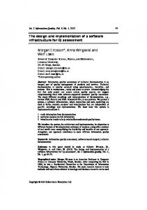
2.2.1.1. SLOPING BAR-CODE A method of using beacons consisting of bar-codes was investigated for the self-localisation system for the SENARIO wheelchair. The commercially available bar-code reader obtained from Symbol Technologies Ltd had a limited minimum and maximum bar-code size that could be read at any particular distance. To obtain a bar-code that could be read over a greater distance, therefore, the reader was angled upwards, and the author developed the sloping bar-code. The sloping bar-code - narrower at the bottom and wider at the top - enabled the bar-code reader to read a narrower code when it was close to the bar-code, and to read a wider code when it was further away, thus keeping the bar-code width within the desired minimum and maximum bar-code lengths. Figure 1 shows a bar-code that could be mounted on a wall and read by a bar-code reader over a larger distance range than if the bar-code were a conventional vertical linear bar-code. The sloping bar-code still has a maximum and minimum reading range distance dependent on the reader system, but this reading range for a vertical linear bar-code is extended using the sloping bar-code.

16

ENVIRONMENT SENSING

Figure 1 - Sloping bar-code to allow the code to be read at increased ranges.

2.2.2. LASER RANGE FINDERS Laser range finders scan their surroundings in two dimensions, providing a range to the nearest object at regular angular increments. Three methods for determining range to an object using a laser range finder are described by Katzberg (1990). The first is time-of-flight, but due to the speed of light accurate detection of short ranges requires sophisticated electronics, which are expensive. The second method uses the phase shift between the transmitted signal and the returned signal to determine the range of the object detected (Shen et al, 1994). The faster the frequency of modulation the easier it is to detect the phase shift for short ranges, but this reduces the maximum range, due to the phase shift being uniquely identifiable only for the first 2π radians of phase shift. The third method is a frequency modulated continuous wave, where the transmitted signal is slowly changed in frequency. The distance to a detected object is then proportional to the

17

ENVIRONMENT SENSING difference in the current transmitted frequency and the received frequency. Clergeot et al (1985) used a modulated range finder on a welding robot application. Laser range finders have inherent errors, measurement noise and limited measurement resolution (Sequeira et al, 1995). A laser beam is a cylinder, and the range measured is the average of the ranges produced at the intersection of the laser cylinder and the surface detected. The area of contact depends on the angle of intersection of the laser beam with the surface normal. A range error is obtained when the laser cylinder comes into contact with more than one object at a reading angle, distorting the edges of objects, thus making their detection harder. The surface reflectance of the object detected distorts the range reading, and brighter objects can appear closer than a darker object at the same distance. There are three advantages of direct range sensing techniques (Sequeira et al, 1995): •

explicit range information is provided without any additional computational overheads;

•

the illumination of the scene does not affect the range data; and

•

the reflectance of the surface detected does not greatly affect the reading received (Shen et al, 1994).

Laser range finders have been used for localisation in a number of diverse ways. Forsberg et al (1995), Tani (1996), Skrzypczynski (1998) and Lawitzky (1999) extracted features from the vector of ranges received, while Armstrong et al (1995) used range finders around the environment in a manner similar to global vision. Pampagnin et al (1995) detected highly reflective beacons using a range finder.

18

ENVIRONMENT SENSING

2.2.3. VISION SYSTEMS Both single camera (Wilkes, 1994) and twin camera (Brady, 1992) vision systems have been extensively used, and Weckesser et al (1995) used three cameras. Vision systems are used to extract either predetermined known (Iñigo & Torres, 1994), or self-taught features from the environment (McKee et al, 1994), which are then used for triangulation or for wall following. Once a feature has been realised from the view, orientation can be calculated and, with multi-camera systems or a multi-position single camera, range to features calculated. Vision-based range finding techniques can be divided into three categories: contrived lighting, passive image-based and multiple images (Jarvis, 1983). Evans et al (1992) used a structured light method by which two light beams reflected off the area in front of an AGV allow the images received by a camera image to be monitored for obstacles. Atiya & Hager (1993) used a camera system to detect vertical edges within the environment and determined the location of an AGV by matching the detected edges to a model of the environment using the least-squares technique. Similarly Schmitt et al (1999) used off-board processing to match the vertical edges produced by a simulator and vertical edges gathered by an on-board camera. An initial location accurate to ±10cm and ±5° was required to ensure that the vertical lines that were being matched were likely to be within the field of view. The method was only tested with a single 15m wall and no unmapped obstacles. Cameras placed throughout the robot’s environment is another vision technique used for mobile robot localisation, where the AGV’s location and navigational commands are determined remotely. This ‘Global Vision’ method, where position and navigational decisions are made centrally, allows for low cost robots to use a relatively expensive

19

ENVIRONMENT SENSING localisation system, thus reducing the cost of the overall system for a multi-AGV application (Kay & Luo, 1992). Brady (1992) and Greenway & Deaves (1994) used global vision to track two radio-controlled cars, with ultrasonic and infrared sensors added to improve the position estimates of the cars. Camera systems have been used in a wide variety of other ways, often to detect specific features. Stella et al (1995) used a single camera system to detect passive reflective beacons around the environment, and then used triangulation to determine the location of the AGV, having been provided with a starting location. Bayer et al (1995) used a camera system to detect lines within their operational environments. They processed the image data off-board the robot and transmitted back to the robot navigational instructions to follow a line painted onto the floor. Asensio et al (1998) used a camera system to determine the location of doorways within an environment by detecting striped tape that had been placed around the doorframe. They then knew their local relative location, and could use this information to navigate towards the door. Zingaretti & Carbonaro (1998) used a binocular camera system to detect known natural landmarks within the environment, such as emergency exit signs, heating vents on walls and ventilation grills in the ceiling. Having been provided with a starting location they were able to navigate their robot around an environment consisting of corridors. Not everyone has been keen to use a vision system, however, not only because of the financial cost, but because camera systems require computationally intensive processing (Flynn, 1988; Bourhis & Pino, 1996). In response to the problems associated with vision systems, such as the need for simplified, relatively static, controlled environments and high performance computing, Brady (1992) designed a stereo camera system for use on an AGV for navigation through narrow gaps among moving obstacles. The system was capable of

20

ENVIRONMENT SENSING camera movements of 530°s-1 and accelerations of 7000°s-2, and was controlled by a transputer for each of the four degrees of freedom, and by an additional supervisory transputer.

2.2.4. ULTRASONIC SENSORS The time-of-flight measurement of an ultrasonic signal from a transmitter to a receiver is directly proportional to the distance between the transmitter and receiver. The transmitted sound, however, is not a single pulse but a chirp that has duration. This duration causes distance errors, as the first echo may not have originated from the first pulse. In the worst case, the first received echo is the last transmitted pulse, an error proportional to the length of the chirp is observed (Flynn, 1988). Bilgiç & Türksen (1995) found that uncontrollable false readings could come from the absorption and specular reflection characteristics of the material detected by the ultrasonic signal. Durieu et al (1989) found that in industrial environments sonar systems do not operate reliably for ranges greater than 2m. Due to specular reflections from obstacles being detected by other receivers, Curran & Kyriakopoulos (1995) poled each of 16 sets of ultrasonic sensors sequentially, rather than receive the data in parallel. Drumheller (1987) swept an ultrasonic transceiver through 360° to obtain a sonar contour of 100 ranges of the robot’s surroundings. However, he found that it is virtually impossible to obtain a useful approximation of a room outline from a single position, because usually only a small portion of a room is visible from a single position and range finder readings often contain extremely large errors due to false reflections. Galles (1993) used ultrasonic sensors to recognise natural landmarks from the environment, using 16 ultrasonic and 16 infrared sensors evenly positioned around a robot.

21

ENVIRONMENT SENSING The ultrasonic data vector was shifted until the largest range was the first range in the vector of ranges, thus the importance of the orientation of the robot was minimised. This technique was investigated in section 4.4.2.2.1. Figueroa & Mahajan (1994) used a transmitter on the robot and receivers throughout the environment, in a similar manner to global vision, to determine the location of the robot. Their system was robust, but required extensive modification of the environment and removed autonomy from the robot, as navigation was determined off-line.

2.2.5. OTHER SENSORS The Global Positioning System (GPS) provides a latitude and longitudinal position with height above sea level to an accuracy of 2m. When using the position received at a known GPS receiver, called differential GPS (DGPS) the accuracy is improved to 1m. Mar & Leu (1996) used DGPS to determine a car’s position within a town environment. They accommodated for a loss of signal, from either the satellites or from the differential transmitter, by including a model matching system from an environment map and an odometry backup. Russell (1995) developed an odour sensor that was capable of detecting an odour placed on a floor. This allowed an odour-sensing and obstacle-avoiding robot to navigate within the environment without needing to learn the environment in which it was placed, without a map and without model matching or triangulation. Floreano & Mondada (1996) placed a single light source in the corner of a robot’s environment. The robot was able to learn to navigate towards the light when it needed to recharge its batteries. Bishop et al (1995; 1998) have developed a 15-element light sensor

22

ENVIRONMENT SENSING connected to an N-tuple weightless artificial neural network with a similar aim of determining the direction required to navigate to a recharging station. Mataric (1990) and Stella et al (1998) used a flux gate compass to determine the orientation of an AGV. However, flux gate compasses are susceptible to magnetic interference within the operational environment (Stella et al, 1998), and are therefore unsuitable for a hospital environment. While Pampagnin et al (1995) used a gyroscope to determine the orientation of their AGV.

2.2.6. FEATURE EXTRACTION Feature extraction as discussed in section 1.1.1.2 is a method of pre-processing the sensor data into a suitable format for the localisation method. Some of the difficulties of feature extraction for different sensor types are discussed here. Feature extraction on visual or range data has the same restrictions as a line-of-sight beacon system: the features must be detectable for self-localisation to be achievable. Unless it can be guaranteed, at all times, that sufficient features will be detectable to determine the vehicle location, then feature extraction cannot be used for reliable self-localisation. The data provided by the range finders is in the form of a vector of range data, where the number of ranges provided by the sensor sets the size of the vector, which can be more conveniently termed a range vector. The features that can be extracted from this range vector - are internal corners, external corners and flat wall segments. An internal corner is detected by a steep local maximum range value (Figure 2a), while an external corner provides a steep local minimum range value (Figure 2b) and a straight wall section is

23

ENVIRONMENT SENSING signified by a constant rate of change of range values, which will produce a local minimum value if the AGV is perpendicular to the wall (Figure 2c).

24

ENVIRONMENT SENSING

Range (cm)

a) Internal corner: 3000 2500 2000 1500 1000 500 0 0

45

90

135

180

225

270

315

360

270

315

360

270

315

360

Angle (degrees)

Range (cm)

b) External corner: 3000 2500 2000 1500 1000 500 0 0

45

90

135

180

225

Angle (degrees)

Range (cm)

c) Straight wall: 3000 2500 2000 1500 1000 500 0 0

45

90

135

180

225

Angle (degrees) Figure 2 - Range vectors for different environment features.

25

ENVIRONMENT SENSING Structured man-made environments are usually uniform in a vertical plane for a sufficient height for most AGV applications (Cox, 1991). Note needs to be taken of features that may not be detected - such as the wall above a door frame, for example - due to the height at which the range finder scans the environment. In the case of autonomous wheelchairs, which may need to drive partly under a table, the uniformity cannot be generally assumed. In a hospital environment other pieces of equipment, sometimes expensive, do not follow the vertical uniformity assumption: portable X-ray machines, or a pull-up handle mounted above a bed are examples. It should be possible to feature extract from ultrasonic data, however due to some of the reflection problems previously discussed in section 2.2.4 it is not possible to reliably detect environment features from ultrasonic range and heading data.

2.3. SENSOR SELECTION FOR SELF-LOCALISATION OF A WHEELCHAIR IN A HOSPITAL ENVIRONMENT Sensors used on an autonomous wheelchair in a hospital environment must be capable of reliably locating the wheelchair and must be acceptable to the user (Napper & Seaman, 1989). From the foregoing review of the literature, and from practical trials with sensors, the sensors chosen as the most suitable for self-localisation of a wheelchair in a hospital environment were a laser range finder and passive radio beacons, backed up by odometry.

2.3.1. SENSORS REJECTED

2.3.1.1. PASSIVE BEACONS A line-of-sight passive beacon system was rejected, as it could not be guaranteed that a minimum of three beacons would always be visible to allow triangulation. Also in a

26

ENVIRONMENT SENSING complex multi-room environment it can be difficult to accurately measure where a beacon has been placed. In the case of bar-code beacons, they also needed to be within the reading range of the reader system.

2.3.1.2. ACTIVE BEACONS Due to electrical installation and regular maintenance requirements this type of beacon was rejected. Line-of-sight active beacons were rejected for the same reasons as those for passive beacons.

2.3.1.3. VISION SYSTEMS In a hospital, a vision camera system mounted on the wheelchair or around the environment, may be perceived as an “eye” on the patients and is therefore unacceptable in this application. Napper & Seaman (1989) emphasise that sensor acceptance is a key consideration when using robots for heath care applications. On-board vision system would also require feature extraction, additional lighting or beacons.

2.3.1.4. ULTRASONICS Ultrasonic sensors were rejected due to the variation in received value from different surfaces and the long range readings required from the operational environments (section 4.1.1).

2.3.1.5. OTHERS GPS localisation was rejected because it is not possible to detect satellites in an indoor environment (pers. obs.). Another problem with GPS is that the orientation is not determined until the vehicle has moved, which means that the navigation system has to determine a free space then move into it before the direction of movement relative to the environment can be determined.

27

ENVIRONMENT SENSING An odour laying and following system is not suitable as the robot needs to be free ranging and a hospital environment is cleaned regularly.

2.3.1.6. FEATURE EXTRACTION The difference between feature extraction and beacons is in the method of obtaining the currently visible feature set. Hence, the same problems found with line-of-sight beacons apply to feature extraction; at least three features must be detectable, and the locations of these features, within the operational environment space, able to be derived.

2.3.2. SENSORS ACCEPTED The sensors that were finally selected for the self-localisation system on the SENARIO wheelchair were two laser range finders, each covering 180°, passive radio beacons and optical encoders. The range finders determined the distances from the wheelchair to the surrounding environment. The passive radio beacons indicated the region of the environment in which the wheelchair was situated. The odometry provided a location estimate while a location was being determined from the range finder and radio beacon data.

2.3.2.1. LASER RANGE FINDERS The advantages of using an active range finder, rather than a passive technique like vision or triangulation, are that an explicit range vector is provided without any additional computation, the illumination of the scene does not affect the range data, and the reflectance of the surface detected does not greatly affect the reading received (Shen et al, 1994). Jarvis (1983) stated that the problems found in some vision based range finding, such as occlusion and reduced accuracy with distance, are solved using laser range finders. The transmitted signal axis and received signal axis coincide, and range accuracy is maintained 28

ENVIRONMENT SENSING while a reliable signal can be detected. Laser range finders, he states, could potentially eliminate the problems found with many sensors. Erwin Sick GmbH manufactured the chosen laser range finders. These provided the longest range, the highest angular resolution, and the most accurate range readings, and had a laser classification of 1, providing high quality data and allowing them to be used in a public place without causing injury from the laser beam. A comparison of alternative range finders that were investigated is given in Appendix A. The laser range finders provided 720 range readings taken at every 0.5° from the wheelchair. The range finders had a specified range error of ±50mm, and a maximum detection range of 50m. The only pre-processing that was required of the range data was to compensate for the separation distance between the centres of rotation of the two range finders. The range finders measure the range to the nearest object at a given angle; this may or may not be an expected range. The self-localisation technique used on the wheelchair needed to be robust to noise. It therefore needed to be able to accommodate changes in the environment, or differences between the expected environment and that detected by the range finders. These perceived differences were treated as input noise to the self-localisation system. To check the manufacturer’s specified range error, the range finders were tested by comparing the ranges output and the ranges measured to a smooth non-painted piece of wooden chip-board placed in front of the range finder. A total of 45 tests were performed at 8 distances between 695mm and 5224mm Table 1.

29

ENVIRONMENT SENSING

Position Number of trials Actual range (mm) Mean range error (mm) Standard deviation 1 2 3 4 5 6 7 8

5 5 4 4 7 6 7 7

695 2319 2695 2735 3092 3931 4737 5224

27.0 23.0 27.5 27.5 52.3 40.7 47.3 21.1

4.5 25.9 5.0 15.0 27.6 4.1 24.4 8.8

Table 1 - Results of range tests on a range finder. Figure 3 shows the distribution 16

of range errors for all 45 range

14

tests and shows that over the

Frequency

12

test ranges the range is likely to

10 8

be over-estimated by 40mm.

6 4

The range readings were not

2

modified to remove the mean

0 -30

-10

10

30

50

70

90

Error values (mm)

Figure 3 - Distribution of range errors when testing the range finders.

error value, as error was small compared to the size of the SENARIO trial environments.

2.3.2.2. PASSIVE BEACONS Passive radio beacons were selected to overcome room location ambiguities derived from the environment consisting of many rooms of the same physical dimensions. Passive radio beacons were chosen as they required no electrical installation or maintenance and can be visually obscured. The installation did not have to be accurate as they were intended only as room identifiers, and not as triangulation markers.

30

ENVIRONMENT SENSING A hospital environment may contain many rooms of identical horizontal profile, which would generate the same input range vector from the range finders. The positioning system would be able to produce a local position only within such a room, but would be unable to provide an exact environment position within the map. This failure would occur irrespective of the method used to determine the location from the range vector. Hence, another system was required to determine which room the wheelchair was in when the current room produced the same horizontal profile as another within the wheelchair environment. It was not desirable to modify the environment, and the SENARIO system was designed to have all control systems on-board the wheelchair. The system used to solve this problem was a passive radio frequency beacon system (TIRIS from Texas Instruments). The passive radio beacons were inductively coupled devices that received their power via a transceiver aerial. The beacons were positioned at known locations around the environment, required no electrical installation, no maintenance and could provide a unique code, or a number of beacons could be given the same code, to indicate no-entry areas. The installation did not have to be accurate as the beacons were intended only as room identifiers, and not as triangulation markers.

2.3.2.3. ODOMETRY The localisation system was made reliable by having odometry available to provide a location estimate if the range finder method failed, or to extrapolate from the previous range finder determined location, until a new location could be accurately determined. Odometry data was used to extrapolate a location from the estimate provided by the range finder data. The wheelchair navigation unit (section 3.2.1) used the extrapolated location when a location was not available from the localisation system.

31

ENVIRONMENT SENSING

2d Lo y^

y L

i

ri

θ

y~ y

θ

θ^

θ x^

x

~ x

x

Figure 4 - Odometry calculation.

Figure 4 shows how a new location could be calculated from the odometry data received from the two drive wheels (Holenstein & Badreddin, 1994; Wang, 1988). In Figure 4, 2d is the separation between the two odometry wheels, Lo is the measured distance travelled by the left-hand wheel and Li is the measured distance travelled by the right-hand wheel. The starting location of the mid-point between the two odometry wheels is given as (x,y,θ). The

(

)

finishing location is identified as x , y ,θ . Given that the length of an arc is rθ, and hence Lo = (2d + ri )θˆ and Li = riθˆ , we can determine the length ri =

2dLi from the odometry measurements, and the angle θˆ from Lo − Li

Li = riθˆ , and then θ . To determine the new x position, we know that the length

32

ENVIRONMENT SENSING

xˆ + ~ x = (ri + d )Cos θ and ~ x = (ri + d )Cosθ so using xˆ = ( xˆ + ~ x) − ~ x then the change in the

x

position

is

(

)

xˆ = (ri + d ) Cosθ − Cosθ .

~ y + yˆ = (ri + d )Sinθ

(

and ~ y = (ri + d )Sin θ

Similarly

with

the

y

co-ordinates,

so the change in the y co-ordinate is

)

yˆ = (ri + d ) Sinθ − Sinθ .

ONCLUSIONS.

2.4. C

The sensors chosen for the AGV were: two 180° laser range finders manufactured by Erwin Sick GmbH, that are now a standard sensor on AGVs (Schofield, 1999); passive radio beacons; and encoders (Beattie, 1995; Beattie et al, 1995; Katevas et al, 1997). The laser range finders were chosen as the primary environment perception sensor for their high angular resolution, their large range, the pre-calculated range data, and their class 1 laser rating. The passive radio beacons were selected to differentiate between similar environment locations perceived by the range finders. They were chosen for their zero maintenance and minimal installation requirements. Encoders mounted against the main AGV drive wheels provided a backup method for determining the current location from the previous location provided by the localisation network. Chapter 3 details the SENARIO wheelchair and section 3.4.1 discusses how the selected sensors were installed. Chapter 4 discusses a number of artificial neural networks that attempted to solve the self-localisation problem using the sensors selected here, hence the networks chosen needed to be able to accommodate the data provided by these sensors.

33

THE SENARIO PROJECT

3.THE SENARIO

PROJECT

NTRODUCTION

3.1. I

This chapter discusses SENARIO, the project that the self-localisation system was tested on (Beattie, 1995; Beattie et al, 1995; Katevas et al, 1995; Katevas et al, 1997). The integration of the self-localisation system on the SENARIO wheelchair project is described in detail in Chapter 6. The SENARIO project was funded by the European Union under the Technology and Innovation for the Disabled and Elderly (TIDE) scheme. The project initiated the need for a new robust self-localisation method, and was used to evaluate, in two non-simulated environments, the FSDN, the novel artificial neural network self-localisation method introduced in Chapters 5 and 6 of this thesis. The objective set for SENARIO was to develop a market orientated prototype wheelchair that could be used by those people who want assistance to move around within a predefined indoor area. The project was aimed at those people who were unable to drive a conventional joystick controlled powered wheelchair. It was designed to be an add-on to existing powered wheelchairs, and as such a Meyra ‘Sprint’ model wheelchair (Figure 5) was used as the base. Having an add-on design allowed manufacturers to consider more easily the design for inclusion in their range as it could be supplied as an optional extra without having to modify their existing production line.

34

THE SENARIO PROJECT

3.1.1. THE WHEELCHAIR A restriction placed on the SENARIO project by the TIDE office was that the autonomous navigation system must use the M3S

bus

protocol.

communication

Hence

wheelchair

the

Meyra

company

was

chosen, as it was possible to have its chairs converted to use the

M3S

bus.

communication Figure 5 – The Meyra wheelchair, used as the SENARIO chassis.

The bus

M3S was

developed from the Controller Area

Network

(CAN)

automotive industry communication bus, for use on wheelchairs by a previous TIDE project (Van Woerden, 1993). The Meyra sprint model wheelchair (Figure 5) has independently driven large rear wheels and free castors at the front. This configuration was selected because it allows for a tighter turning circle than the Meyra Genius model wheelchair, which has front wheels that are driven in tandem with steering rear wheels. However, the free front castors on the ‘Sprint’ wheelchair caused navigation problems as they caused the wheelchair to deviate from the desired path of travel until the castors turned into a trailing orientation.

35

THE SENARIO PROJECT

3.1.2. OPERATION The SENARIO wheelchair was designed to have two operating modes. The first mode, termed ‘semi-autonomous’, allowed a user to drive the chair in a desired direction while offering protection from collision with static or dynamic obstacles. However, the user was restricted to travel only at the wheelchair’s minimum speed when overriding safety limits. The user controlled the chair using voice commands for four directions of motion, ‘forward’, ‘backward’, ‘left turn’ and ‘right turn’. If obstacles could be avoided, the chair continued in the requested direction until stopped by the user. By specifying a goal location, the user controlled the second ‘fully-autonomous’ mode of operation. The wheelchair determined its current location and planned a global path to the requested location. During travel, local obstacles were avoided and progress was monitored by continuously recalculating the current location.

UB-SYSTEMS

3.2. S

The wheelchair consisted of four sub-systems, which were centred around the Risk Avoidance sub-system, as shown in Figure 6. The Sensing and Positioning sub-systems connected directly to the Risk Avoidance sub-system, while the Control Panel and Power Control sub-systems were connected through the M3S bus. This allowed the SENARIO system to be constructed to control any wheelchair that has the M3S communication bus, and for alternative user interfaces to be attached to suit user requirements. This section describes the Risk Avoidance, Sensing, Control Panel and Power Control sub-systems. The Positioning sub-system is described in more detail in section 3.3.

36

THE SENARIO PROJECT

Control panel Sub-system

Positioning Sub-system

Risk avoidance Sub-system

Sensing Sub-system -

Power control Sub-system

Figure 6 – The SENARIO control system structure, consisting of four sub-systems connected to the Risk Avoidance system.

The Risk Avoidance sub-system was developed by the SENARIO project co-ordinators, Zenon SA a Greek automation company; the Sensing sub-system was developed by MicroSonic GmbH, a German ultrasonic sensor manufacturer; the Control Panel sub-system was developed by the Institute of Communication and Computer Science at the National Technical University of Athens; the Power Control sub-system was developed by the French National Institute of Health and Medical Research INSERM Unit 103; and the Positioning sub-system was developed by the author under the guidance of Dr Mark Bishop of the Department of Cybernetics at the University of Reading.

3.2.1. RISK AVOIDANCE SUB-SYSTEM Zenon were responsible for the Risk Avoidance sub-system, which provided overall control of the wheelchair. The sub-system monitored for the following external risks using the Sensing sub-system’s devices: obstacles, high speeds and holes; it also monitored for sensor, actuator or communication failures as internal risks.

37

THE SENARIO PROJECT

As overall controller, the Risk Avoidance sub-system contained the navigation unit. The unit consisted of two parts, a global and a local path planner. When the wheelchair was being operated in the ‘fully-autonomous’ mode, the global path planner received the current wheelchair location from the Positioning sub-system and determined a suitable route to the desired goal location, which was received from the user interface in the Control Panel sub-system. The global path planner, having selected a route to the goal location, produced a list of intermediate goal locations. The local path planner then monitored for local obstacles and determined a route between the global path intermediary goal location, passing the drive commands via the M3S bus and the Power Control sub-system to the drive motors.

3.2.2. SENSING SUB-SYSTEM The Sensing sub-system developed by MicroSonic GmbH was responsible for monitoring the local environment for obstacles. The major sensors were ultrasonic, mounted around the wheelchair in the directions that it was possible for the wheelchair to manoeuvre. Three groups of ultrasonic units were used. The first group were two sensors at the front of the wheelchair pointing downwards to detect whether a floor was present in front of the wheelchair. These sensors detected if the wheelchair was about to attempt to drive down a hole or a stairway. The second group of sensors were used to detect distant obstacles around the wheelchair and provide information to the local navigation unit. The final group of ultrasonic sensors were approved for personal protection by the European authorities. When this final group of ultrasonic devices sensed an obstacle that was too close to the wheelchair they (independently from the navigation unit) stopped the wheelchair motors. The five personal protection ultrasonic sensors (Microsonic Sonarshultz) were mounted at the front and back of the chair. One at the back prevented the wheelchair from reversing

38

THE SENARIO PROJECT

into any obstacle; the other four were mounted at the front of the chair, two horizontally and two inclined at an angle of 45°. The inclined sensors prevented the chair from colliding with obstacles that were not uniform in the vertical plane, such as tables. The six ultrasonic sensors used for navigation were mounted at the corners and sides of the wheelchair. The corner units were mounted at 45° with respect to the central axis of the wheelchair, and the side units were mounted at 75°. These angles allowed the navigation system to monitor for obstacles in the regions in which it may have wished to turn. Although it used fail-safe ultrasonic sensors to prevent the wheelchair from colliding with any obstacle, the system also had an additional contact bumper added to the wheelchair to detect any physical contact between the outermost frame of the wheelchair and an obstacle.

3.2.3. CONTROL PANEL SUB-SYSTEM Developed by the National Technical University of Athens, the Control Panel sub-system used voice recognition and a joystick to receive user commands. Voice recognition was selected for control of the wheelchair as it was believed to permit the largest possible number of potential users to use the wheelchair. The voice recognition unit was taught to recognise both the semi-autonomous commands and the fully autonomous goal location commands of an individual user. The voice recognition unit was capable of recognising 160 commands with the available memory, though the number of recognisable commands could have been increased with more storage memory. However, the time delay to respond to a specific command increased with the number of stored commands.

39

THE SENARIO PROJECT

3.2.4. POWER CONTROL SUB-SYSTEM INSERM unit 103 were responsible for the Power Control sub-system. This system translated the drive requests from the navigation system into commands sent on the M3S bus to each of the drive wheels.

OSITIONING SUB-SYSTEM

3.3. P

The Positioning sub-system, which this thesis details, was responsible for providing the navigational unit with the current wheelchair location in terms of its position and orientation, allowing the progress of the wheelchair to be monitored as it travelled through the operational environment. As the wheelchair could be switched on at any place in the environment, the system had to be able to self-locate without any user input. The self-localisation method developed (Chapters 5 & 6) used the fixed environment walls to determine the wheelchair location. The two laser range finders that the system used for this purpose were mounted on an arch above the user, so that they were more likely to detect environment walls than furniture or other non-modelled items. The system had two modes of operation. Firstly, with information only from the range finders, it needed to determine the current position and orientation of the wheelchair. Secondly, given an initial location estimate plus the information from the range finders, it needed to provide an updated location estimate. In the second mode it was not necessary for the system to interrogate the entire environment area to determine the current location, rather it was necessary only to investigate a sub-section of the environment map. The self-localisation system that was developed had to provide the navigation unit with a global environment position and orientation, not a location within a current room. This task became difficult when the relative positions of the walls in more than one room were the

40

THE SENARIO PROJECT

same, thus making it impossible to determine which room the wheelchair was occupying from the room’s walls alone. To solve this problem, passive radio beacons were added to rooms that were the same shape, to provide a unique identification to these rooms. The passive radio beacon system is explained in more detail in Chapter 6, where the installation of the self-localisation system onto the SENARIO wheelchair is described.

3.3.1. CONSTRAINTS ON THE POSITIONING SUB-SYSTEM The SENARIO wheelchair was designed for use in an operational rehabilitation centre, where it would have been extremely inconvenient to disrupt the operation of the centre by installing free ranging AGV tracking systems such as global vision or active beacons. Because many people visited the environment, camera systems were not considered appropriate, as they would be perceived as monitoring devices. Maintenance of the system needed to be as low as possible, so an active beacon system was also unsuitable, because regular checking would be necessary to ensure the robust operation of the system. The need to use a wheelchair with the M3S communication bus installed restricted to two the choice of wheelchair that could be used. As a result, the wheelchair design was not suitable for direct mounting of sensors, and a metal framework had to be built around the base and above the user. The size of the sensor frame was limited to ensure that the wheelchair would fit through doorways, both from a height and width perspective. Using a wheelchair, however, provided freedoms to the system that would not be available on a smaller AGV. There were no restrictions, as far as the Positioning sub-system was concerned, on the battery supply duration when the SENARIO autonomous system was installed. Only one microprocessor was permitted for each of the Risk Avoidance and Positioning sub-systems. Due to the scale of the project, the cost allowed for sensors was

41

THE SENARIO PROJECT

large, and the weight of the sensors was unrestricted due to the size of the wheelchair, and its capacity to pull heavy loads.

3.3.2. POSITIONING SUB-SYSTEM COMMUNICATIONS The communications system used on the Positioning sub-system is shown in Figure 7 (section 3.4.2). It consisted of a PC-104 four port serial board, with the first port connected to the Risk Avoidance sub-system, the second connected to the radio beacon’s controller module, and the third and fourth ports connected to the two range finders. The communication protocols between the Risk Avoidance sub-system and the Positioning sub-system on the wheelchair were finalised during their integration onto the wheelchair. To provide a fast serial communications link between the two systems, a baud rate of 38,400 was used, without a start bit and only one stop bit. To check the integrity of the data transfer, even parity checking was enabled. Hardware handshaking was used, avoiding the need to encode and decode the data, which is required in software handshaking. A buffer of 1000 bytes was ample on the Positioning sub-system for the incoming data, as the number of bytes in each transmission was expected to be a maximum of 20. The Positioning sub-system used interrupts both to detect the presence of incoming data and to output the required data, thus providing the fastest response to the Risk Avoidance sub-system when requests were made, and allowing the transmission of data to be performed when the communication channel became available, while not preventing the execution of other functions while waiting for availability of the channel. Two messages were used with the Risk Avoidance sub-system, one at either end of the operation of the Positioning sub-system. One was at the end of the Positioning sub-system sequence, when it had determined the location of the wheelchair. The Positioning sub-system provided to the Risk Avoidance sub-system the new location information. The

42

THE SENARIO PROJECT

other message was initiated by the Risk Avoidance sub-system, indicating that it would like an updated location estimate based around a location provided by the Risk Avoidance sub-system, this could be the location that had just been provided by the Positioning sub-system. Communications to the radio beacon controller was restricted by the maximum communication speed of the beacon system to a baud rate of 9600, and the protocol used was 8 data bits, one stop bit and no parity checking. Communications to the beacon system, as with the Risk Avoidance sub-system, used interrupts to control the transfer of the data, as this allowed the communications to be performed when the communications channel was available. The Positioning sub-system initiated the beacon system to monitor for a beacon and, if a beacon was detected, the beacon system replied with the beacon’s identification number. The beacon identification number was translated into a predetermined wheelchair position, using a small look-up table that was loaded into the processor memory from a text file at system initiation. The beacon position data file used a simple structure to contain the relevant positional information. The file began with the number of radio beacons that were used in the wheelchair’s environment, and then a list of the radio beacon identification numbers with corresponding x and y environment positions. Communication to the range finders also used interrupts, and were set to the range finders’ default baud rate of 9600 to ensure that communication could always be established when the range finders were switched on. The protocol used was defined by the range finders as 8 data bits, one stop bit and even parity. Each range was received from the range finders as four byte reversed ASCII values. A value of 3, for example, was received as the ASCII value 51dec. This allowed software handshaking, because control characters were not confused with data values. The range value consisted of four digits, received in the order

43

THE SENARIO PROJECT

2nd, 1st, 4th, 3rd. The data received then needed to be divided by the scale factor to correspond with the map scale. The separation between the centres of rotation of the two range finders needed to be taken into account when amalgamating the range data into one contiguous vector of ranges.

NSTALLATION OF THE POSITIONING SUB-SYSTEM

3.4. I

The Positioning sub-system was integrated onto the wheelchair. As has been described in Chapter 2, the Positioning sub-system consisted of the two laser range finders and the passive radio beacon system. In addition there was a processor unit, with hard disk, video card and a four port serial communications board.

3.4.1. SENSOR INSTALLATION The laser range finders were mounted at a height of 192cm on a frame above the wheelchair. This allowed a large number of unmapped obstacles to go undetected by the range finders, and provided a clearer view of the environment walls, which were included in the operational map. This height also permitted the wheelchair to pass clearly through doorways. The passive radio beacon’s aerial was mounted on the underside of the wheelchair. This was intended to provide a maximum range for beacons placed on the floor. However, the range was diminished due to the metal construction of the wheelchair and proximity to the d.c. drive motors. The odometry sensor were installed and the odometry calculations were under the control Risk Avoidance sub-system, as this allowed the navigation system to be developed and tested independently of the Positioning sub-system.

44

THE SENARIO PROJECT 3.4.1.1.

I

NSTALLATION PROBLEMS WITH RADIO BEACONS

Texas Instruments’ TIRIS passive radio beacon system was mounted underneath the wheelchair. The system consisted of an aerial and a control module that communicated to the Positioning sub-system using one of the serial ports. The control module was mounted in a protective box, beneath the wheelchair at the front, which allowed its operation to be easily monitored. The aerial was mounted onto a steel frame, in turn attached to the underside of the wheelchair. The radio beacons could not be tested in operation on the wheelchair for two reasons. Firstly, the power supplied on the wheelchair was unable to provide sufficient power to all the equipment on the wheelchair, so that when the radio beacon controller was switched on, the Risk Avoidance sub-system and Positioning sub-system processors would fail. Secondly, the steel mounting which attached the antenna to the underside of the wheelchair adversely affected the range of the beacons system when tested with only the Positioning sub-system processor being powered.

3.4.2. POSITIONING SUB-SYSTEM CONFIGURATION The Positioning sub-system processor was situated at the left-hand end of the SENARIO control box, and required four back plane slots. Two slots were used for connection: one for the processor and one for the video display card. The video display was necessary only during the programming and integration phases of the project, as no display was provided to the user by the Positioning sub-system during normal operation. The processor, serial communication board and the hard disk were powered from a +5 volts and 0 volt supply. The video card required an additional +12 volt supply. Figure 7 shows the Positioning sub-system’s processor configuration. The processor board communicated to the Positioning sub-system’s sensors, and the navigation unit’s Risk 45

THE SENARIO PROJECT

Avoidance sub-system using the four port serial card. The PCMCIA hard disk connected into the processor’s IDE hard disk controller port.

2 Infrared Scanners

Risk Avoidance

PC104 four port serial board

Pentium 200Mhz Processor

PCMCIA Hard Disk

Radio Beacons

Figure 7 - Positioning sub-system configuration.

3.4.3. MEMORY Originally, 8 Mbytes of memory were specified for the requirements of the Positioning sub-system. This was sufficient to prove the operation of the algorithm developed for SENARIO’s localisation requirements (Chapters 5 and 6). In order to improve the speed of the algorithm, however, it became necessary to pre-process the environment map (section 4.3.1.1). Map pre-processing was used to determine which walls were visible from any position within the environment. Thus, rather than having to calculate measurements from all walls, the Positioning sub-system calculated only the measurements from the list of ‘visible’ walls for the specified position. The size of the data structure to contain all the pre-processed wall information required a considerable amount of room, however, both in terms of disk space for the file containing the pre-processed data and RAM to hold the run time pre-processed data. Consideration was given to holding the data structure on the hard disk and not loading it into RAM; this would have greatly increased the time required to retrieve the pre-processed data, however, and so was rejected. The maximum amount of memory that could be installed onto the processor system was purchased. However during 46

THE SENARIO PROJECT

the integration phase it became apparent that even when using the maximum amount of memory possible on the system (64 Mbytes) the pre-processed map data structure would not fit into the memory available. Thus it was necessary to scale the environment map. A scaling factor was used by the map pre-processor and the localisation programme to signify how many centimetres a unit of range represented.

3.4.4. HARD DISK A removable PCMCIA hard disk was used, as a single floppy soon became insufficient when using large pre-processed map files. Furthermore the removable hard disk could be used on any standard portable computer, allowing the map pre-processing to be carried out off-line and later transferred to the wheelchair. The unit had the advantages of the size of a hard disk and the convenience of a floppy drive when transferring data to the wheelchair. Connecting the drive to the processor’s IDE hard disk port allowed the system to self-boot from the hard disk directly.

47

THE SENARIO PROJECT

3.4.5. HARDWARE INSTALLATION Figure 8 shows the wheelchair

Range finders

with

the

sensing

and

self-localisation, the

processor

systems installed. The frame around the chair can easily be seen, with the laser range finders mounted on top and all but two of the ultrasonic

Sonarschultz

transducers mounted around the chair, within the contact sensor. The

range

finders

were

mounted onto a hollow tubular, Obstacle detection ultrasonics

straight-sided steel frame over the wheelchair. Each range

Bumper Figure 8 - Wheelchair with the Positioning sub-system installed.

finder was secured at the bottom,

using

manufacturer’s

the mounting

holes, by three bolts onto a mounting plate welded to the top of the arch. The range finders were then attached to each other, again using the manufacturer’s mounting holes, on both sides using steel plates and four securing bolts. Each range finder used a dedicated serial port on the Positioning sub-system processor and shared a +24 volt power supply.

48

THE SENARIO PROJECT

UMMARY OF CONTROL SYSTEMS INSTALLED

3.5. S

The Sensing, Control Panel, Power Control, Risk Avoidance and Positioning sub-systems were successfully integrated to the wheelchair. The Positioning sub-system consisting of two range finders and a passive radio beacon system were interfaced to the Positioning sub-system’s processor system, which communicated location information to the Risk Avoidance sub-system.

49

ARTIFICIAL NEURAL NETWORK SELF-LOCALISATION

4.ARTIFICIAL NEURAL NETWORK

SELF-LOCALISATION NTRODUCTION

4.1. I

This chapter assesses the suitability of three existing artificial neural networks for solving the self-localisation problem on the SENARIO wheelchair described in Chapter 3. Tests were performed to demonstrate the accuracy and repeatability of the different networks. The testing environment maps and the method used to represent them to the networks are detailed, along with an environment simulator that was used to test the networks. Artificial neural networks were chosen because a model could be developed to translate the range vector received from the range finders into a location only in a trivial environment, without noise. The networks evaluated were: a radial basis function (RBF) (Moody & Darken, 1989), an associative weightless N-tuple network (Beale & Jackson, 1990) and a stochastic diffusion network (SDN) (Bishop & Torr, 1992). These particular networks were chosen as they had been used either in solving positioning problems or for searching for patterns within large search spaces. The N-tuple and SDN were tested using the environment maps that were used to test the SENARIO wheelchair with users. The initial SENARIO test environment was an industrial workshop measuring 1920 × 1813cm with 720 0.5° angles translates to (1920 × 1813 × 720) 2,506,291,200 possible environment locations. The required accuracy for the SENARIO wheelchair was The first network considered was a set of radial basis functions. Such systems have been implemented for positioning by Townsend et al (1994), who pre-processed range finder

50

ARTIFICIAL NEURAL NETWORK SELF-LOCALISATION

data into seven inputs. The implementation tested here used no data pre-processing, providing the network with a 720 dimensional input space, rather than a 7 dimensional input space as used by Townsend et al (1994). The 720 dimensional input space provided a large amount of redundancy, and prevented the problem that Townsend found where one single range value error corrupted three of the seven RBF input values (Townsend & Tarrassenko, 1999). To provide an output of three dimensions (x,y,θ), three separate basis function networks were required on for each dimension, each being presented with identical input data. The second network, an N-tuple associative weightless network, was taught a subset of rotationally invariant environment positions. This network was considered for its speed of operation and simple implementation. It required a considerable amount of memory, however, and could identify only the positions that it had been taught, and could not interpolate between them. Finally, a stochastic diffusion network was implemented, as this had been shown to be capable of finding a small data set within a large data set (Bishop & Torr, 1992). The search space was reduced in the N-tuple (section 4.4.2.2), and the stochastic diffusion network (section 4.4.3), (and the focused stochastic diffusion network introduced in Chapter 5), by removing the angular information from the range data provided by the range finders, thus dividing the search space by the angular resolution of the range finders, in our case, 720. Townsend et al (1994) suggested that if their RBF network was to be capable of determining a position in real time it was important that the input to the network be rotationally invariant. The operation, implementation and test of the SDN is discussed in detail in section 4.4.3.

51

ARTIFICIAL NEURAL NETWORK SELF-LOCALISATION

4.1.1. NETWORKS NOT IMPLEMENTED A Kohonen self-organising feature map and a Multilayer Perceptron (MLP) network were considered, but not implemented, for the reasons detailed below. A Kohonen self-organising feature map is a classifier network (Beale & Jackson, 1990). It operates by constructing a mapping between a continuous input space and a discrete n-dimensional rectangular output space (Haykin, 1994; Sarle, 1997). The locations of the neurons within the output space are learnt by modifying the locations of a set of the closest current neurons towards the input vector. Implementing this network for the self-localisation problem is impractical for the following reasons. First, the network would need to be taught every single location within the operational environment, and these would need to be presented repeatedly to enable the network to determine output clusters. Second, each of the clusters that the network learnt would have to be manually identified as a particular environment location (Beale & Jackson, 1990). Bearing in mind that there are 2.5 billion locations in the Zenon environment (see section 4.1.1), training and labelling times would seriously limit any practical self-localisation application. Finally, the Kohonen network uses the full range vector as its input, and therefore any noise within critical parts of the input vector could cause the wrong cluster to be activated. When applied to the self-localisation problem, the network would be particularly intolerant of noise in the input space because each individual location would be very similar to that of its neighbour, making it hard for the network to differentiate between noise and an adjacent location. The Multilayer Perceptron network can be trained using back propagation, by presenting inputs and the required output to the network, and adjusting the weights of the network to reduce the error between the current output and the desired output (Beale & Jackson, 1990;

52

ARTIFICIAL NEURAL NETWORK SELF-LOCALISATION

Haykin, 1994). This network was also considered impractical for the self-localisation problem. Firstly, the network would be very large, requiring an output for each location within the operational environment. Secondly, the network would take a restrictively large amount of time to train, again requiring multiple presentations of each environment location. Both the Kohonen self-organising map and the Multilayer Perceptron networks classify every possible point within the output space (environment), and so need to be taught a perturbed version of the input vector for every output point several times for these networks to learn to classify the output points (Haykin, 1994). The perturbations made to the input vectors need to include some that are large and applied to a sequence of adjacent input elements, so that the networks can learn to accept inputs representing an obstacle that may be near to the wheelchair, as well as noise introduced by the range finder. The time to train both the Kohonen self-organising map and the MLP networks would be considerable. For example: given that the number of locations that the networks need to learn to classify is 2,506,291,200 for the Zenon environment, and supposing that 25 training patterns were required for each classification, and that it took half a second for each iteration, (run the simulator, perturb the input, and adjust the network weight), then this would take 996 years to teach the network one environment.

EST ENVIRONMENTS

4.2. T

A building environment may be considered at two levels: either as a whole environment or as a collection of individual rooms and corridors. The environments were considered as a whole, because the range finders could detect mapped features in other rooms or corridors

53

ARTIFICIAL NEURAL NETWORK SELF-LOCALISATION

when doors were open. This offered the advantage that only one map was necessary rather than a collection of maps that needed to be co-ordinated to cover the whole environment.

Data File structure. Maximum X Maximum Y value Minimum X value Minimum Y value Number of walls value wall 0 (X1,Y1)(X2,Y2) wall 1 (X1,Y1)(X2,Y2) wall 2 (X1,Y1)(X2,Y2) wall 3 (X1,Y1)(X2,Y2) wall 4 (X1,Y1)(X2,Y2)

Data File 300 250 0 0 5 00 000 000 000 250 01 000 250 300 250 02 300 250 300 000 03 300 000 200 000 04 100 000 000 000

Figure 9 - Environment map and associated data file. The environment was represented to the networks as a data file that contained the environment dimensions and the number of walls. The data file then continued to detail the co-ordinates of the end points of each straight wall segment in the environment. Figure 9 shows a trivial environment and the associated data file structure required. Figure 10, Figure 11 and Figure 12 show the three test environments that were used for the desktop trials performed in this chapter.

54

ARTIFICIAL NEURAL NETWORK SELF-LOCALISATION 190

centimetres

140

90

40

-10 -10

40

90

140

190

240

290

centim etres

Figure 10 – The 55-Walled test environment map, with the environment walls shown in blue. Figure 10 shows a fictitious 55-Walled environment that contains many similar rooms and also two long corridors. These environment features were chosen to test how the networks would cope with multiple locations with similar or identical features. The origin for the environment is in the bottom left hand corner and increases in the x dimension to the right and in the y dimension upwards. The environment ranged from 0 to 280units in the x dimension and from 0 to 180units in the y dimension.

55

ARTIFICIAL NEURAL NETWORK SELF-LOCALISATION

centim etres -100

400

900

1400

1900

0

centim etres

-500

-1000

-1500

-2000

Figure 11 – The Zenon test environment map, with the environment walls shown in blue. Figure 11 shows the ‘Zenon’ environment. This real environment was used to initially test the SENARIO wheelchair, and it was therefore used in the desktop trials to allow comparisons between the different networks. The environment contained 48 walls, but was much larger than the 55-Walled environment. The short lines and crosses within the map represent girders that supported the roof. The environment’s origin is in the top left hand corner, with the y-dimension decreasing in a downward direction, to allow compatibility with the navigation system on the SENARIO wheelchair. The environment range was from 0 to 19.20m in the x dimension, and 0.37 to -17.76m in the y dimension.

56

ARTIFICIAL NEURAL NETWORK SELF-LOCALISATION

-100

400

centim etres 900 1400

1900

2400

100

-400

centim etres

-900

-1400

-1900

-2400

Figure 12 – The Rehabilitation Centre environment map, with the environment walls shown in blue. Figure 12 shows the Rehabilitation Centre environment map, which contained 107 walls and was larger than the Zenon environment. This real environment consisted of one long corridor, three major rooms and a stairwell, but the wheelchair could not access three areas in the environment. The environment range was from -0.16m to 20.98m in the x dimension and 0 to -21.46m in the y dimension.

It was not possible for the maps used by the simulator to contain all static environment features. For example, the Zenon trial site contained an open slatted staircase, which was (inconsistently) transparent or opaque to the range finders, depending on the wheelchair’s location. The map contained only static obstacles, and in the case of the Zenon trial site, 57

ARTIFICIAL NEURAL NETWORK SELF-LOCALISATION

did not contain half a car, a Puma 700 robot, or a forklift truck, nor the many visitors who stood around the wheelchair.

VALUATION SIMULATOR

4.3. E

A range finder simulator was developed as part of the network system used to determine the location of the wheelchair. The simulator produced range values using simple wall segment environment maps as shown in Figure 10 to Figure 12. The simulated range vectors were then used to represent the range vector that would be produced by the wheelchair’s range finders, or it was used by some of the tested networks (section 4.4.3 and Chapter 5) to produce simulated range vectors of possible resultant locations.

Figure 13 – Position simulation display for an ideal square room environment.

58

ARTIFICIAL NEURAL NETWORK SELF-LOCALISATION

The position simulation display (Figure 13) shows the range values produced by the simulator within a small square environment. This graph was produced from an ideal environment where there were no unmapped obstacles. The local maxima are the corners of the room and the local minima are the perpendicular distances to the four walls. The orientation is shown on the horizontal axis from 0° to 359.5° and the range on the vertical axis from 3 to just over 9 units.

4.3.1. SIMULATOR OPERATION The simulator operated as follows (Table 2). A master range vector was initialised to the maximum possible range in the current environment. Each wall’s ranges were calculated and if the corresponding range values were less than those in the master range vector, then the master vector was overwritten with the shorter range. Thus, the master range vector finally contained the shortest ranges from a given (x,y) position. The orientation was fixed at 0° during the range calculations, but simple shifting of the range vector provided any desired orientation.

Angle 0 30 60 90 120 150 180 210 240 270 300 330

Wall 1 Range Vector 5000 5000 5000 5000 20 40 60 65 5000 5000 5000 5000

Wall 2 Range Vector 100 90 80 70 60 5000 5000 5000 5000 5000 5000 110

Wall 3 Range Vector 5000 5000 5000 5000 5000 5000 5000 80 70 60 50 55

Wall 4 Range Vector 300 200 190 185 250 300 5000 5000 5000 5000 5000 5000

Master Range Master Range Vector Vector Rotated by 120° 100 90 80 70 20 40 60 65 70 60 50 55

70 60 50 55 100 90 80 70 20 40 60 65

Table 2 - The simulator range vector is the shortest range calculated for each wall for each angle, and orientation is set by rotating the range vector.

59

ARTIFICIAL NEURAL NETWORK SELF-LOCALISATION

The procedure to determine the ranges from the range finders’ simulated position to the walls given in the environment map is described below. 1. Set the master range vector to the maximum range for the environment. 2. For each wall: i. Determine the equation of the wall ( y = a + bx ). ii. Set the wall’s range vector to a maximum. iii. Determine the perpendicular distance between the wall and the simulated range finder position. iv. Determine the distance from the simulated range finder position to the start co-ordinates of the wall. v. Determine the distance from the simulated range finder position to the stop co-ordinates of the wall. vi. Determine the angle of the wall’s start position with respect to 0° at the simulated range finder position. vii. Determine the angle of the wall’s stop position with respect to 0° at the simulated range finder position. viii. Determine in which angle quadrant (0-90,90-180,180-270,270-360) the wall’s start position is and determine if the wall’s stop position is clockwise or counter-clockwise around the range finder position. This sets whether the ranges are calculated by incrementing or decrementing through the range vector array. ix. Determine the array element that corresponds to the angle of the wall’s start position angle. x. Determine the array element that corresponds to the angle of the wall’s stop position angle. xi. Test whether the start and stop angles of the wall are equal; if so, set the range to the wall at this angle equal to the lesser of the two ranges. xii. For each array element between the start array element and the stop array element, calculate the range to this wall. 3. Over-write the final range vector with the values from each wall’s range vector if the value is less than the current value in the final range vector.

The above method ensures that the ranges from the walls that can be ‘seen’ by the simulated position over-write the ranges from walls that cannot be ‘seen’ at each of the 720 angles. 4.3.1.1.

P

RE-PROCESSING FOR THE SIMULATOR

The calculation time required to determine a range finder simulation was proportional to the number of walls in the environment, when using the above method. To improve the run-time calculation time, the map was pre-processed using a quad-tree (Kambhampati &

60

ARTIFICIAL NEURAL NETWORK SELF-LOCALISATION

Davies, 1986) to determine which environment walls were visible from each position within the environment, allowing only the walls that were required to calculate the range vector to be used by the simulator for a particular location, rather than testing all walls for all locations. The environment was initially divided into four, and each position in it was sequentially tested: if the walls that could be seen from all positions within that quarter were not identical, then the area was repeatedly divided by four until all positions within the current quarter contained the same walls (Figure 14). As each angle was tested to determine which wall was visible at that angle, the maximum number of walls needed to calculate the final range vector was the angular resolution of the range finder. The preprocessor thus determined which walls needed to be tested by the simulator to produce a range vector, preventing it from testing walls that were not visible from the position being simulated. Pre-processing

of

the

map

produced a large data file, which to improve speed was loaded into

memory

when

the

localisation network program was initialised. However, the data file was too large for the processor

system

memory

installed on the wheelchair when using a 1cm resolution map, so a Figure 14 - Environment division using a quad-tree to determine which walls can be detected from every position. The environment walls are shown as blue lines and the quad-tree division lines as black.

scaling factor was introduced to reduce the resolution of the map

61

ARTIFICIAL NEURAL NETWORK SELF-LOCALISATION

and allow the pre-processed data to be loaded, further details are given in section 6.2.2.

RIAL NETWORKS

4.4. T

Three networks were tested using simulated range data to determine if they could be implemented successfully on the SENARIO wheelchair: the RBF, associative N-tuple network and stochastic diffusion network. These were chosen to represent a radial basis function, an associative memory network and a search network. Their operation, construction and testing in simulated environments and the results of these trials are described below.

4.4.1. RBF The RBF network was chosen because Townsend et al (1994) had previously shown that it could return the position of a mobile robot within an indoor environment. They taught their RBF network to classify a set of features obtained from range vector data. In our case (discussed further in section 4.4.1.2) we wanted to retain the in-built redundancy within the range vector, and therefore used the range vector directly and taught the network to create clusters for the x output space dimension, which then provided a single x dimension output value. 4.4.1.1.

RBF

OPERATION

The learning process for an RBF requires only a single iteration to determine the weight coefficients required to generalise the network output for a particular topology of basis functions. However, considerable time is required for the system to test and compare different configurations and to determine the optimum topology (Haykin, 1994). The network structure consists of an input sensing layer, a second layer of hidden units of a suitably large number, and an output layer providing the desired result to the input layer.

62

ARTIFICIAL NEURAL NETWORK SELF-LOCALISATION

The transformation between the input and hidden layer is non-linear, while the transformation between the hidden layer and the output layer is linear. Over’s theorem states that a non-linear mapping can be used to transform a non-linearly separable classification problem into a linearly separable one (Haykin, 1994). Two phases of operation are then required. The training phase in which, given a set of input to output patterns, a fitting procedure is implemented that produces a surface in the hidden layer’s high dimensional space. The second phase is the generalisation phase, in which interpolation is performed between the data points and the surface produced in the first phase (Haykin, 1994). An RBF network attempts to determine the function that simultaneously transforms a set of N input vectors to their corresponding outputs. Given that Xi are the input vectors and di are their corresponding outputs, then the interpolation condition is the function F that satisfies the condition: F(Xi) = di , where i = 1,2,3,...,N. The RBF technique specifies that the function should take the following form: F(x) =

å w ϕ( x − x ) N

i

i

i =1

The individual radial basis functions,

{ϕ ( x − x ) i = 1,2,..., N }, i

are a set of N arbitrary non-linear functions where the norm is generally the Euclidean and the known input vectors are the centre of the functions. The weight vector wi is the linear factor of the interpolation, and the xi are the centres of the radial basis functions (Haykin, 1994).

63

ARTIFICIAL NEURAL NETWORK SELF-LOCALISATION

The centres may be placed throughout the multi-dimensional hidden layer space using a number of methods. They may be placed randomly, uniformly or using the k-means method, which places the centres at the most significant points in the search space. The kmeans algorithm minimises the sum of squared errors of each of the randomly or uniformly placed k clusters. The RBF network is divided into two stages, learning and operating: In the learning stage the network learns the required output by selecting the position of the radial basis function centres and by determining the weights required to sum the radial basis function results to produce the network outputs. The centres are positioned using the k-means algorithm, which takes some time, as the number of centres used is user selected. Hence the learning process tests an increasing number of centres and tests the network using a set of sample inputs and outputs to determine which number of centres gives the minimum output error. The weights used in the summation of the radial basis functions to produce the output are determined by having several input and output values and using simultaneous equations to solve the output equation, A = wi F ( x )i In the operating stage the network is initially loaded with the input data. The centre coordinates from the learning process are then used to configure the network. The linear output weights are then loaded, and final output values calculated. The first step calculates the output of the hidden layer, which always contains a radial basis that operates on the norm between the centre and the input. Hence the norm value is always calculated and passed to the b-splines radial basis function. The outputs from the hidden layer nodes are F (x ) =

å d ln d N

2 i

i

i =0

64

ARTIFICIAL NEURAL NETWORK SELF-LOCALISATION

where N is the number of centres and d is the Euclidean distance between the origin and the point specified by the input vector. The M hidden layer outputs are then multiplied by a weight factor and summed to produce the final output. A=

å w F (x ) M

j

j

j =0

4.4.1.2.

RBF

APPLIED CONSTRUCTION

A single RBF was constructed using the 720 range values received from the simulation of the range finders as the input vector, with the output being the x axis co-ordinate. It would have been necessary to construct an additional two structures for the y and θ co-ordinates to use RBFs to fully locate the wheelchair. To produce the least error, using sample data from every 5cm across the environment, 240 centres were required. Five centimetres was chosen as a compromise resolution (reducing the time and data that would be needed for one centimetre resolution). 4.4.1.3.

RBF

TESTING

The RBF network was tested using a simple 4-walled, square, 100cm by 100cm environment, and the positional results in the x dimension were tested for an accuracy greater than ± 1cm. Only a small environment and one dimension were used, as the memory and time required to determine the number of centres was prohibitive. The maximum number of centres which gave the best performance when determining the number of centres using the least squares algorithm was 245. 4.4.1.4.

RBF

RESULTS

Figure 15 shows that as the number of centres within the RBF that were used to locate the x dimension increased, the mean positional error and the standard deviation decreased.

65

ARTIFICIAL NEURAL NETWORK SELF-LOCALISATION

Absolute positional error in X (cm )

3 2.5 2 1.5 1 0.5 0 0

50

100

150

200

250

300

-0.5 Num ber of centres

Figure 15 - Variation in error with the number of centres used in the RBF.

4.4.2. ASSOCIATIVE N-TUPLE NETWORK The N-tuple artificial neural network is very simple in its operation and hence is comparatively fast compared with the large RBF network. The N-tuple network is designed to be very fast to teach and to operate, requiring only a single pass to test each taught position, but is capable only of giving a probability that the input is one that has been taught, and is not easily able to interpolate between taught positions (Beale & Jackson, 1990). One N-tuple class/position discriminator can be trained to recognise one position in an environment. Thus to determine the position of a wheelchair a set of such discriminators must be mapped over the operational environment. 4.4.2.1.

N-

TUPLE OPERATION

The range vector input was connected to the address lines of a number of simulated Random Access Memories (RAMs). The number of address inputs to each RAM determined the sensitivity of the network to noise. The more RAMs that were used, the fewer address lines were required on each RAM to cover the input area. The fewer RAMs that were used, the more sensitive the network was to noise. RAMs operate using binary inputs; hence the range values were not immediately compatible and needed to be 66

ARTIFICIAL NEURAL NETWORK SELF-LOCALISATION

converted to binary values by passing them through Minchinton cells (Bishop et al, 1991). Minchinton cells are two value comparators that produce a binary TRUE value if input a is greater than input b; and in all other cases a FALSE value is produced. The range values were selected for comparison by the Minchinton cell from a repeatable random sequence before being presented as binary inputs to the RAMs. The sequence of random range values was retained, as the same sequence was required when running the network. To ensure that all elements were selected, an array containing all the index values was used and elements randomly swapped in pairs to produce a random ordered array of all the index values. The array was then used sequentially. Each RAM was presented with an input onto its address lines generated from the output of the Minchinton cells. During the learning phase the selected address was activated and a TRUE value stored there. As long as the network was not saturated during learning it is unlikely that all possible addresses will be presented to each RAM. Another set of RAMs was then taught a new input pattern. This continued until the whole input was suitably covered with discrete taught positions (Figure 16).

67

ARTIFICIAL NEURAL NETWORK SELF-LOCALISATION

RAM RAM Minch Cell

RAM RAM

Minch Cell

Figure 16 - Random connection of Minchinton cells to the input data, which are then connected to a RAM. Only one RAM’s connections are shown for clarity.

The larger the tuple size the more testing points were connected to each RAM and hence the fewer RAMs were necessary to entirely cover the area to be tested. Thus the larger the tuple size the more accurate the input must be for a match to be found, so the less noise the network can accommodate, but the fewer false positive results will be found. 4.4.2.2.

N-

TUPLE APPLIED CONSTRUCTION

An N-tuple network was constructed with a tuple size of four, as this allowed for a reasonable amount of tolerance to noise while not requiring too much memory (memory use increases as the tuple size increases). The software implementation of the network was built around a three-dimensional array, in which the first two dimensions were the number of discrete x and y positions required to 68

ARTIFICIAL NEURAL NETWORK SELF-LOCALISATION

cover the environment map. The third dimension was the number of RAMs used for each position discrimination. The value held at each location in the array was the address value presented to the RAM. In operation the network presented the RAMs with address inputs that had been passed through Minchinton cells. The data contents of the selected address of each RAM were tested. The number of RAMs that contained an active address was an indication of the probability that the input pattern matched the taught patterns for these RAMs. The RAMs for all the different taught positions were tested and the position that had the most active RAMs was the position with the greatest probability of being correct. 4.4.2.2.1.

ROTATIONAL INVARIANCE

In the self-localisation application the output of the network was the discrete taught positions, rather than any interpolation between taught positions being provided. The network treated a rotation of a position as a new position and hence would need to be taught each desired angle, which would make the number of taught positions very large. To reduce the locations that were required to be taught to the network the system was made rotationally invariant to the wheelchair location. However, this also meant that it could not estimate the orientation. The technique that was tried on the N-tuple network used the largest range as reference. This ‘largest range’ technique required that a simulated range vector be produced for the position determined by the network. The input and the simulated vectors were then rotated until the largest range elements in each vector were first. The largest element was used because the shortest range detected by the wheelchair would probably be an obstacle. The search then provided the (x,y) position and the angle was the simulated vector shift minus

69

ARTIFICIAL NEURAL NETWORK SELF-LOCALISATION

the input vector shift. This worked well with noise free data but if the longest vector was obscured then the (x,y) position would not be found, and the search would fail. The second approach that was investigated was termed the ‘range histogram’ technique. This method created a frequency histogram of the ranges obtained from the range finders, by taking a count of a number of adjacent range values. The number of range columns within the range histogram was fixed at 200. Thus the width of each column, or the spread of range values counted by each column, was determined by dividing the maximum range that could be obtained within an environment by the number of columns (200). This gave column widths of 5cm for 55-Walled, 30cm for Zenon and 35cm for the Rehabilitation Centre environments. An example range histogram is shown in Figure 22. The longest range technique was used for the N-tuple network as calculation was very fast and accurate when using simulated range vectors for range finder input. 4.4.2.3.

N-

TUPLE TESTING

The N-tuple network was tested using three maps: the fictitious 55-Walled test map and the two SENARIO test environment maps of Zenon and the Rehabilitation Centre. The test positions used were generated using the simulator (section 4.3). Thus, the input data was ideal, and all environment features were effectively included in the model and the environment was noise free. The tests on the three environments consisted of 84 trials each. Each trial tested 30 different locations, with six of these locations being tested ten times. The trials were undertaken to demonstrate how well each network performed in terms of the accuracy of the resultant location, to ± 1cm and 1°, and the repeatability of the location determined.

70

ARTIFICIAL NEURAL NETWORK SELF-LOCALISATION

The 55-Walled map used a maximum range of 340cm, a histogram width of 5cm and a tuple size of 4. The number of learnt positions was on a grid, where the map was divided by 100 on both the x and y axes, with the x axis ranged from 0 to 280cm and the y axis ranged from 0 to 180cm. The Zenon environment, being larger, required a maximum range of 2640cm, with a histogram width of 30cm. The x axis range was from 0 to 1920cm, the y axis range was from 37 to –1776cm, and the tuple size was 4. The learnt positions were the grid of points found by dividing the x and x axes by 200. The Rehabilitation Centre environment, being even larger, required a maximum range of 3000cm and a histogram width of 35cm. The x axis range was from –16cm to 2098cm and the y axis range was from 0 to –2146cm, with a tuple size of 4. As with the Zenon map the learnt positions were determined by dividing the environment by 200 in the x and y axes. The histogram column width and the maximum number of divisions in the x and y dimensions affected the amount of memory required, and these values were set to the highest resolution that would fit within the 80 Mbytes of memory available on the desktop computer. 4.4.2.4.

N-

TUPLE RESULTS

Figure 17, Figure 18 and Figure 19 show the individual positional results of the N-tuple network in the three test environments. The standard deviation (SD) results that are given below are for the repeated test locations that were used to determine if the network was repeatable.

71

ARTIFICIAL NEURAL NETWORK SELF-LOCALISATION 190

Location F

140

centimetres

Location A

90

Location B 40

Location D Location C Location E

-10 -10

40

90

140

190

240

290

centimetres

▲

g

Figure 17 – N-tuple location results using the 55-Walled environment map. The ( ) represent the positions being tested and the ( ) show the position calculated using the N-tuple network. The (─) show the (x,y) Euclidean error between the test and derived positions. The named locations refer to the repeated test positions.

Figure 17 shows the N-tuple results using the 55-Walled map. The mean (x,y) Euclidean error was 75.9 ± SD 69.5cm, while the mean (x,y,θ) Euclidean error was 271.0 ± SD 174.6cm° (Figure 20 and Figure 21). In this environment the results for the (x,y) and (x,y,θ) trials, used to test the repeatability of the network, had a standard deviation of 0, that is they were perfectly repeatable.

72

ARTIFICIAL NEURAL NETWORK SELF-LOCALISATION centimetres -100

400

900

1400

1900

0

Location A Location E

centim etres

-500

Location F

Location D

-1000

Location B

Location C

-1500

-2000

▲

g

Figure 18 - N-tuple location results using the Zenon environment map. The ( ) represent the positions being tested and the ( ) show the position calculated using the N-tuple network. The (─) show the (x,y) Euclidean error between the test and derived positions. The named locations refer to the repeated test positions.

Figure 18 shows the N-tuple results using the ‘Zenon’ map. The mean (x,y) Euclidean error was 92.1 ± SD 296.2cm, while the mean (x,y,θ) Euclidean error was 345.4 ± SD 320.7cm° (Figure 20 and Figure 21). Again the results for the (x,y) and the (x,y,θ) trials, used to test the repeatability of the network, had a standard deviation of 0.

73

ARTIFICIAL NEURAL NETWORK SELF-LOCALISATION centim etres -100

400

900

1400

1900

2400

100

Location A

-400

Location B

Location C

centim etres

-900

Location D -1400

Location E

-1900

Location F

-2400

▲

g

Figure 19 - N-tuple results using the Rehabilitation Centre environment map. The ( ) represent the positions being tested and the ( ) show the position calculated using the N-tuple network. The (─) show the (x,y) Euclidean error between the test and calculated positions. The named locations refer to the repeated test positions.

Figure 19 shows the N-tuple results when using the Rehabilitation Centre environment map. The mean (x,y) Euclidean error was 268.9 ± SD 393.2cm, while the mean (x,y,θ) Euclidean error was 455.3 ± SD 343.7cm° (Figure 20 and Figure 21). Again the results for the (x,y) and the (x,y,θ) trials, used to test the repeatability of the network, had a standard deviation of 0. In all environments the mean (x,y) Euclidean error was always less than or equal to the mean (x,y,θ) Euclidean error, as the orientation error was always greater than or equal to

74

ARTIFICIAL NEURAL NETWORK SELF-LOCALISATION

zero. The Euclidean errors were largest in the Rehabilitation Centre environment, because the best fit solutions were a large distance, compared to the other environments, from the desired position, even if the location was very similar (Figure 20). The mean (x,y) Euclidean errors for all test locations were mostly small, with one and three particular exceptions in the Zenon and Rehabilitation centre environments respectively. The network was perfectly repeatable with zero standard deviations for all repeated test location trials using the N-tuple network (Figure 21).

75

ARTIFICIAL NEURAL NETWORK SELF-LOCALISATION 1000

Mean (x,y) Euclidean error (cm)

800

600

400

200

0 Walls 55

Zenon

Rehabilitation Centre

-200

-400 Test Environm ent

1000 900

Mean (x,y,theta) Euclidean error (cm°)

800 700 600 500 400 300 200 100 0 Walls 55

Zenon

Rehabilitation Centre

Test Environm ent

θ

Figure 20 – The N-tuple mean [(x,y) top and (x,y, ) bottom] Euclidean errors for all trials.

76

ARTIFICIAL NEURAL NETWORK SELF-LOCALISATION loc A

loc B

loc C

loc D

loc E

loc F

1400

Mean (x,y) Euclidean error (cm)

1200 1000 800 600 400 200 0 Walls 55

Zenon

Rehabilitation Centre

Test Environm ent 1400

Mean (x,y,theta) Euclidean error (cm°)

1200 1000 800

600 400 200 0 Walls 55

Zenon

Rehabilitation Centre

Test Environm ent

θ

Figure 21 – The N-tuple mean [(x,y) top and (x,y, ) bottom] Euclidean errors with standard deviations for the repeated test locations.

4.4.3. STOCHASTIC DIFFUSION NETWORK The Stochastic Diffusion Network (SDN) can be used to locate a predefined data pattern within a given search space (Bishop & Torr, 1992). It is a global best-fit search technique and as such will not converge to a local minima (Bishop, 1989; Nasuto & Bishop, 1999).

77

ARTIFICIAL NEURAL NETWORK SELF-LOCALISATION 4.4.3.1.

SDN

OPERATION

When the term position is used within this section it refers to a data element within the search space and not the (x,y) position of a wheelchair within an environment. The SDN operates in parallel using a pre-defined number of elements called agents, each characterised by its activity (firing or not-firing), and a pointer to a position in the search space (Bishop & Torr, 1992). The network can be considered as a competitive co-operative process in which all agents independently seek solutions. Once an agent finds a solution, it competes for a greater allocation of network resources. A solution with a better fit to the data model has a higher chance of attracting more agents than other solutions. In this way competition transforms smoothly into co-operation, as more and more agents are attracted to explore a potential fit to the data model. This competition for co-operation ensures that all potential positions of the object within the search space will be examined independently with the most promising one, over a number of iterations, attracting most of the computational resources. Thus the correct position of the best fit to the data model will emerge from independent, parallel exploitation of different potential positions in the search space, by gradually disregarding less accurate matches. From this principle it follows that agents will cluster over interesting positions in the search space as soon as the first agents pointing to these positions spread information to others (Nasuto & Bishop, 1999). The network operation involves several stages and can be summarised in the form of the following algorithm (Beattie & Bishop, 1997; Beattie & Bishop, 1998): INITIALISATION PHASE WHILE NOT TERMINATION TESTING PHASE DIFFUSION PHASE TEST TERMINATION CONDITIONS END WHILE

78

ARTIFICIAL NEURAL NETWORK SELF-LOCALISATION

Assigning random positions or mappings to the agents in the search space performs the initialisation phase. During the testing phase, positions pointed to by agents are evaluated by comparison of a randomly chosen subset of system inputs produced by a simulator. If the comparison is successful the agent becomes ‘active’; otherwise it remains ‘inactive’. During the diffusion phase, positions of active agents can cross to inactive agents. Each ‘inactive’ agent randomly selects another agent in the network and copies its search space mapping if active, or simply re-selects a location at random if not. Hence, the mapping contained by active agents defines possible solutions. This may or may not, however, be the globally correct solution. The probability that an agent's solution is correct, rather than a false positive, increases with each iteration that the agent remains active. The longer that an agent remains active the higher the probability that inactive agents will select it and acquire its mapping. It has been shown that without noise the solution will rapidly diffuse to all agents (Nasuto & Bishop, 1999). The process iterates until termination conditions are fulfilled. Bishop & Torr (1992) proposed the following equilibrium-based termination condition: if the number of agents pointing to the same position within the search space exceeds a given threshold and remains constant within specified bounds over a number of iterations, then the network may be said to have reached equilibrium and the solution is the mapping selected by these agents. Where all agents are randomly selecting a position within the search space and mappings are not being diffused from successful agents, the probability of SDN selecting the correct solution in the first iteration of the network can be determined by:

79

ARTIFICIAL NEURAL NETWORK SELF-LOCALISATION P = 1 − (nq n −1 p )

Where P = the probability of selecting the correct location, n = the number of agents, p = 1 / number of locations, q = 1 - p. 4.4.3.2.

SDN

APPLIED CONSTRUCTION

A SDN was constructed in which agent mappings were initially uniformly randomly selected from the (x,y,θ) environment search space. The simulator produced a range vector for the system location that the agent had defined, and by comparing a number of these simulated ranges with the current input ranges from the range finders, the agent mappings were tested. It was not necessary to test all the elements of the range vector due to the redundancy of the input data (Townsend et al, 1994). An agent was defined as ‘active’ if all the differences between the input and agent ranges were within a predetermined fixed tolerance (20cm). To increase the speed of the network, the task of determining the location was split in two: first, to determine the position using rotationally invariant inputs; and second, to determine the orientation. Once the position had been determined, all agents were set to test the same position at randomly chosen orientations. Thus, the simulator needed to be run only once to produce the range values and the agents rotated the vector to obtain the orientation they had each selected. The range histogram approach for rotational invariance (section 4.4.2.2.1) was used.

80

ARTIFICIAL NEURAL NETWORK SELF-LOCALISATION 250

Frequency

200

150

100

50

0 1

51

101

151

Range column number Zenon (1600,-100)

Figure 22 - An example range histogram from an input range vector.

To test each agent’s position solution, a comparison was made between the histogram produced from the agent’s range vector simulator and the histogram produced from the input range vector. An example of an input range vector histogram is shown in Figure 22. Not all columns within the histograms were tested; the more columns that were tested the harder the overall test became, and the more likely the test was to correctly fail incorrect positions. The columns that were tested at each iteration were chosen randomly each time for all agents. If the frequency within the same columns of the two graphs was within a tolerance value for all columns that were being compared, then the test was successful, and the agent was set to active. The maximum range detectable by the range finder, and the tolerance required, determined the number of columns used in the histograms. As with the N-tuple version, each column represented the frequency of a group of range values from the range vector. For each column there was a lower and upper range value, Figure 22 shows a range vector histogram from the Zenon environment where the column width was

81

ARTIFICIAL NEURAL NETWORK SELF-LOCALISATION

30cm. If a low resolution was required then each column contained a wide range of range values. To obtain a higher resolution a narrower range of values was covered by each column. When a lower resolution was used, any changes in range were smoothed out, so the more likely the test was to pass incorrect locations. Orientation testing compared six individual range values from the input and agent range vectors, and the agent was set to active if they were within 20cms of each other. The angles that were tested were randomly chosen each time for each agent. 4.4.3.3.

SDN

TESTING

A 1000-agent SDN was used to test the three environments: 55-Walled, Zenon and the Rehabilitation Centre. Three parameters caused the network to terminate its searching: the number of iterations, the minimum number of active agents, and the change in the number of active agents. The number of iterations before termination was set to 10,000, at which point the network was assumed not to have been able to determine a solution. For comparison, the mean number of iterations for the 55-Walled, Zenon and Rehabilitation Centre was 44, 329 and 185 respectively, suggesting that this termination condition was suitable. The minimum number of active agents was greater than 100 to prevent the network terminating due to the number of active agents not changing while the network was attempting to find initial correct solutions. To ensure that the network had settled to a reasonably stable state at termination, the number of active agents must not have changed by more than 20 in the last four iterations. The test positions discussed were all simulated. Thus, the input data were ideal, and all environment features were effectively included in the model and the environment was noise free.

82

ARTIFICIAL NEURAL NETWORK SELF-LOCALISATION

The tests on the three environments were the same as the N-tuple network tests: 84 trials performed using 30 different locations, with six of these locations tested ten times. Again the trials aimed to demonstrate the network’s performance in terms of accuracy, to ± 1cm and 1°, and the repeatability. During the testing phase of the SDN a tolerance was permitted between the ranges calculated by the agent’s location being tested and the input range vector from the range finders’ simulated range. A trial was performed to determine the effect of varying this tolerance value. Fifty trials were performed at the same location within the 55-Walled simulated environment for four different tolerance values, (18,15,13 and 11cm) using 1000 agents. The trials recorded the Euclidean positional and locational errors, the number of iterations taken until convergence upon a solution, and the number of active agents at convergence. 4.4.3.4.

SDN

RESULTS

This section details the results obtained when testing the network in the three different simulated test environments at the same locations as the previous network trial, and the results obtained from varying the acceptance tolerance.

83

ARTIFICIAL NEURAL NETWORK SELF-LOCALISATION 190

Location F

140

centimetres

Location A

90

Location B Location D 40

Location C

-10 -10

40

90

Location E

140

190

240

290

centimetres

g

Figure 23 - SDN results using the 55-Walled test environment map with simulated test positions ( ) and their results ( ), joined by Euclidean errors (─). The named locations refer to the repeated test positions.

▲

The results for the 55-Walled environment were very poor (Figure 23). However, consideration needs to be given to the size or resolution of the environment, which was only 280 by 180cm compared with the 2000 by 2000cm (approximately) environments of Zenon and the Rehabilitation Centre, and the fixed tolerance value of 20cm for the three environments. The effects of environment size are discussed further in section 4.4.3.4.1.

84

ARTIFICIAL NEURAL NETWORK SELF-LOCALISATION

centim etres -100

400

900

1400

1900

0

Location A

Location E

centim etres

-500

Location F

Location D

-1000

Location B

Location C

-1500

-2000

Figure 24 - SDN results using the Zenon test environment map with simulated test positions ( ) and their results ( ), joined by Euclidean errors (─). The named locations refer to the repeated test positions.

g

▲

Figure 24 shows the results for the Zenon test environment. It can be seen that the network accurately located 7 out of 15 of the test positions. The individual results of the other 8 test positions have either selected the correct position or a similar environment location. It can clearly be seen that for the unsuccessful positions the network has selected positions that are at symmetrically similar environment positions, as the majority of the Euclidean error lines pass through the centre of the environment. The two lines that do not go through the centre of the environment have selected similar positions within a sub-region of the environment.

85

ARTIFICIAL NEURAL NETWORK SELF-LOCALISATION centim etres -100

400

900

1400

1900

2400

100

Location A

-400

Location B

Location C

centim etres

-900

Location D -1400

Location E

-1900

Location F

-2400

Figure 25 - SDN results using the Rehabilitation Centre test environment map with simulated test positions ( ) and their results ( ), joined by Euclidean errors (⎯). The named locations refer to the repeated test positions.

g

▲

The Rehabilitation Centre environment had many more similar environment locations than the Zenon environment, and so it was harder for the network to select the correct result for this environment (Figure 25). In the few positions that were unique a good result were given - e.g. (600,-1300) and (400,-900). Clearly the test locations at the top left-hand side of the Rehabilitation Centre environment (200,-200) and at the right-hand end of the long corridor (2000,-700) contain many alternative locations, even some that are not physically accessible [e.g. (400,-1150) and (400,-1500)].

86

ARTIFICIAL NEURAL NETWORK SELF-LOCALISATION

Figure 26 shows the (x,y) and the (x,y,θ) Euclidean errors using the SDN on the three test environments. The mean (x,y,θ) Euclidean error was larger than the mean (x,y) Euclidean error, as the orientation error was greater than or equal to zero. The mean (x,y) and (x,y,θ) Euclidean errors for only the repeated test locations (Figure 27) had a larger standard deviation when the error was larger, showing that when the network was not good at determining a result it was not as repeatable.

87

ARTIFICIAL NEURAL NETWORK SELF-LOCALISATION 1200 1000

Mean (x,y) Euclidean error (cm)

800 600 400 200 0 Walls 55

Zenon

Rehabilitation Centre

-200 -400

Test Environm ent

1200 1000

Mean (x,y,theta) Euclidean error (cm°)

800 600 400 200 0 Walls 55

Zenon

Rehabilitation Centre

-200 -400

Test Environm ent

θ

Figure 26 – The SDN mean [(x,y) top and (x,y, ) bottom] Euclidean errors for all trials.

88

ARTIFICIAL NEURAL NETWORK SELF-LOCALISATION loc A

loc B

loc C

loc D

loc E

loc F

2000

Mean (x,y) Euclidean error (cm )

1500

1000

500

0 Walls 55

Zenon

Rehabilitation Centre

-500 Test Environm ent

2000

Mean (x,y,theta) Euclidean error (cm °)

1500

1000

500

0 Walls 55

Zenon

Rehabilitation Centre

-500 Test Environm ent

θ

Figure 27 – The SDN mean [(x,y) top and (x,y, ) bottom] Euclidean error with standard deviations for the repeated test locations for the three trial environments.

89

ARTIFICIAL NEURAL NETWORK SELF-LOCALISATION

4.4.3.4.1.

RANGE VECTOR HISTOGRAMS

The poor performance of the SDN in the 55-Walled environment (Figure 23) can be explained by examining typical SDN range vector histograms (4.4.2.2.1) from each of the environments (Figure 28). These typical range vectors from the three trial environments show that for the 55-Walled and the Rehabilitation Centre environments the utilised ranges were generally shorter than for the Zenon environment, where the ranges had a more even distribution of short and long ranges.

90

ARTIFICIAL NEURAL NETWORK SELF-LOCALISATION 250

Frequency

200

150

100

50

0 1

51

101 Range column number 55-Walled (150,30)

151

101

151

250

Frequency

200

150

100

50

0 1

51

Range column number Zenon (100,-1100)

250

Frequency

200

150

100

50

0 1

51

101 Range column number Rehabilitation Centre (1000,-700)

151

Figure 28 – Typical range histograms for the three trial environments. 91

ARTIFICIAL NEURAL NETWORK SELF-LOCALISATION

Figure 29 shows that the locational Euclidean errors for all SDN trials within all three test environments were affected by the distribution of the ranges across the range vector histograms. With the exception of position [Zenon (1600,-100)], when the area of the range vector histogram greater than 50 was more than 100 then the locational Euclidean error increased.

2500 Zenon (1600,-100)

(x,y,theta) Euclidean error (cm°)

2000

1500

1000

500

0 0

50

100

150

200

250

300

350

400

450

Area of the range vector histogram graph greater than 50

θ

Figure 29 – The (x,y, ) Euclidean error versus the number of range vector histogram columns with a frequency greater than 50 in each trial range vector histogram.

A value of 50 was chosen as the threshold for measuring the area above the threshold, as from the examples in Figure 28 the majority of columns are less than this threshold. The network developed in Chapter 5 attempted to overcome this problem by dynamically changing the number of columns within in the range vector histogram during the evaluation of a location.

92

ARTIFICIAL NEURAL NETWORK SELF-LOCALISATION

4.4.3.4.2.

TOLERANCE VALUE To test the effect of changing the tolerance value, a small test environment was constructed consisting of a square room inside

a

(Figure 30).

square The

room

effects

of

varying the tolerance value can be seen in Figure 31 and

Figure 30 - Tolerance value test environment.

Figure 32.

The

data

points

shown are for the number of correct agents, the number of iterations and the Euclidean errors, for four different tolerance values (18, 15, 13 and 11). Figure 31 shows that the number of active agents at termination decreased as the tolerance value decreased, whilst the number of iterations required until termination is achieved increased. The error bars indicate the standard deviation of the sample of 50 trials, and show that the number of active agents at termination became more constant as the tolerance value decreased. The standard deviation error bars show that the number of iterations required to obtain a solution varied more as the tolerance value decreased. This is dependent on how few iterations were required for the search to obtain the first correct solution that can then be diffused to the other agents. Figure 32 shows that the resultant positional and locational Euclidean errors decreased as the testing tolerance value decreased.

93

800

800

700

700

600

600

500

500

400

400

300

300

200

200

100

100

0

Number of Iterations

Number of agents

ARTIFICIAL NEURAL NETWORK SELF-LOCALISATION

Active agents Iterations

0 18

15

13

11

Tolerance Value (cm)

Figure 31 - Number of active agents at termination and the number of iterations until termination when using different tolerance values when testing agents.

18

Euclidean Error

16 14 12

Euclidean error (x,y,theta) (cm°)

10 8

Euclidean error (x,y) (cm)

6 4 2 0 18

15

13

11

Tolerance Value (cm)

Figure 32 - Positional and locational Euclidean errors when using different tolerance values when testing agents.

ISCUSSION

4.5. D

4.5.1. RBF As the system took four days to determine that 245 centres produced results with the least mean error and the standard deviations with ± 0.5cm, for one dimension in a very small environment, the network was considered impractical for use on the SENARIO 94

ARTIFICIAL NEURAL NETWORK SELF-LOCALISATION

wheelchair. It is noted that Townsend & Tarassenko (1999) used off-board processing, a 4.5m by 5m obstacle free environment and derived a two-dimensional result from their RBF network. The RBF network was too large to be implemented using a 720 dimensional input vector, and a reduced input such as Townsend et al’s (1994) would be required to enable the network to fit within the available memory. However, we wanted to retain the inherent redundancy available within the raw range vector, to allow the system to be able to operate when the input range vector differed from the ideal range vector due to obstacles.

4.5.2. N-TUPLE Comparison of the range vectors produced by the simulator for test and resultant locations in the 55-Walled environment show that the N-tuple network often selected similar environment locations as result locations. For example in Figure 17 the test location at (220,60) was near the right-hand end of the corridor, while the result selected by the network was at (60,60), towards the left-hand end of the corridor, giving an (x,y) Euclidean error of 160. Figure 33 shows that these two simulated range vectors are very similar except for rotation.

95

ARTIFICIAL NEURAL NETWORK SELF-LOCALISATION

Figure 33 - Graphs of the simulated range finder data at the test position (220,60), and the simulated range data from the resultant position (60,60) in the 55-Walled environment. 96

ARTIFICIAL NEURAL NETWORK SELF-LOCALISATION

The N-tuple network was able to provide a result to a resolution dependent on the size of the environment and the number of sample points in each dimension. In the case of the x dimension in the Zenon environment, then the resolution was only 10.49cm (2098/200), while the Risk Avoidance sub-system on the SENARIO wheelchair specified a resolution of 1cm; and so the network was rejected. The N-tuple and stochastic diffusion networks showed similar results: they both performed poorly in the small 55-Walled environment, with the SDN not able to determine any of the trial locations. Both the N-tuple and the SDN performed quite well in the Zenon and Rehabilitation Centre environments. It is noticeable that there is no random element in the N-tuple network and that the results, with ideal inputs, have consequently not varied. In a non-simulated environment with noise, variation would be expected.

4.5.3. SDN The SDN was able to determine the test positions accurately in the Zenon environment, but not accurately in the 55-Walled and the Rehabilitation Centre environments, which had many more environment positions that contained similar subsets of range vectors to that of the position being tested. The positional results shown in Figure 23 appear particularly poor as the width of each column in the range histogram graph was very small, and the frequency of the ranges in the range vector was very low, making the comparison of different range values always within the relatively large tolerance value. This is discussed further in section 4.4.3.4.1. The number of active agents that the network contained at termination decreased and became less variable as the testing tolerance value decreased. This was due to the test being harder and the number of false positive selected locations decreasing. The number of iterations required until termination increased as the tolerance value decreased, due to only

97

ARTIFICIAL NEURAL NETWORK SELF-LOCALISATION

a few agents containing correct solutions, and the diffusion of these few correct solutions requiring more iterations until a minimum number of agents were active. Position and location Euclidean errors reduced as the testing tolerance value decreased. Standard deviation also decreased with a decreasing tolerance value, signifying that the results became more repeatable as well as more accurate. To translate this into an operational system, however, would mean that the time required to obtain a result will increase, but will be more precise. It may therefore be suitable to have a large tolerance value at the early stages to ensure that the system has selected the correct area within the environment, and then to reduce the tolerance value to refine the result. This is the basis of the Focused Stochastic Diffusion Network introduced in Chapter 5.

ONCLUSIONS

4.6. C

The networks that were tested were the RBF, the N-tuple and the SDN. The RBF required a very large network and took a very long time to determine the optimum location of the centres, but its results in a small environment in one dimension were very accurate. The N-tuple network took several hours to be taught a subset of the environment positions. Due to memory limitations only a subset of the environment positions could be taught to the network, and the determination of the orientation was limited. The SDN was accurate in environments without many similar locations. Once the Stochastic Diffusion Network had been demonstrated to have had some success in the simulated environments that the SENARIO wheelchair would operate, the adaptations presented in Chapter 5 were made to improve the speed of the network by making it focus towards the correct solution.

98

FOCUSED STOCHASTIC DIFFUSION NETWORK

5.FOCUSED STOCHASTIC DIFFUSION NETWORK NTRODUCTION

5.1. I

This chapter introduces the Focused Stochastic Diffusion Network (FSDN) (Beattie & Bishop, 1997; Katevas et al, 1997; Beattie & Bishop, 1998) as a novel method to solve the self-localisation problem on an autonomous AGV in a large environment. The FSDN is an extension of the Stochastic Diffusion Network (SDN) described in Chapter 4. In the FSDN the space of possible solutions is explored in parallel using a multi-resolution pyramid by a collection of agents searching in a competitive co-operative manner for the most likely location of an AGV in its environment. As with N-tuple and SDN (Chapter 4) the results are presented for three simulated environments (Chapter 6 shows results from two nonsimulated environments where the FSDN was applied to the SENARIO wheelchair). The structure and operation of the FSDN is described, then its application to solving the self-localisation problem, the method used to reduce the search space size, and the results of trials on the three simulated environments. Finally a comparison is made between the N-tuple, SDN and FSDN networks.

5.2. FSDN

OPERATION

To understand the operation of the FSDN, an understanding of the operation of its predecessor, the SDN, is essential. This is dealt with in detail in Chapter 4, and so is only briefly described here.

99

FOCUSED STOCHASTIC DIFFUSION NETWORK

The SDN consists of a number of agents that randomly select locations within the current search space. Firstly, in the testing phase, each agent in turn requests a simulated input for the search space location that it has selected. Using a fixed tolerance, the agent compares a fixed number of randomly selected columns from its range histogram (section 4.4.2.2.1) to compare against the same columns from the network input range histogram. If all the selected columns are within tolerance then the agent is termed ‘active’, as the location it has selected has passed the position testing phase. The agents then determine the orientation by all agents testing the same position. Once all agents have performed the testing phase, each agent in turn performs the diffusion phase. This phase allows the ‘inactive’ agents to randomly select another agent. If the randomly selected agent is also ‘inactive’ then an entirely new random search space location is selected. However, if the randomly selected agent is ‘active’ then the ‘inactive’ agent acquires its location. This process allows the successful agents to propagate their success to other agents. Unlike the SDN, the FSDN does not attempt to select the correct solution immediately. Rather, it tries to find the area of the search space that contains the correct solution, and then narrows in on the correct solution to produce a final solution. The FSDN extends the SDN in three ways: 1. Each FSDN agent randomly selects a region rather than an exact location (the different types of regions that can be used are discussed in 5.2.1); 2. The FSDN agents compare a variable number of input elements during the testing phase; 3. The FSDN agents use a variable tolerance when testing input elements between those of the agent’s selected location and those produced from the network input.

100

FOCUSED STOCHASTIC DIFFUSION NETWORK

To control the variable tolerance value and the number of elements that are to be tested, a count called the ‘focus level’ represents how successful an agent has been within its current region. The simplest method of controlling the operation of the agent using the focus level value is to decrease the tolerance value and increase the number of ranges tested as the focus level increases. Other methods of controlling the tolerance and number of test angles are discussed later in this chapter.

5.2.1. REGIONS The FSDN does not attempt to find the exact solution. Instead it seeks a region of the search space that contains the solution. The regions initially cover a large area of the network search space, and then are sub-divided as the agent focuses on a correct

solution.

The

search

progresses by using ever-decreasing Figure 34 - Regions sub-division.

region

sizes,

and

reducing

the

comparison tolerance (Figure 34) between the network input and the input provided by the simulator for the agents.

PTIONS AVAILABLE WHEN APPLYING FSDN TO THE SELF-LOCALISATION PROBLEM

5.3. O

A variety of alternative means of configuring FSDN were available. Among the features that could be changed to best suit the self-localisation problem were; the sub-division of the search space, the rate of focusing and the simulator operation.

101

FOCUSED STOCHASTIC DIFFUSION NETWORK

5.3.1. ENVIRONMENT CO-ORDINATE FRAME The

locations

self-localisation

provided

by

the

system

to

the

navigation system of the wheelchair had to be provided in Cartesian coordinate form, although the locations could be represented in any manner within the FSDN. To emphasise this point, the polar co-ordinate system was considered, with the bottom left Figure 35 - Polar co-ordinate method of determining environment regions.

of the search space as the origin. The search space was then divided along

the x-axis and through 90° into sub-regions (Figure 35). This meant that the physical area covered by a sub-region became larger farther away from the origin. This method was rejected for this application, as the probability of a region containing the correct solution was non-uniform and biased towards positions further from the origin. A simple linear division of the environment in the x and y dimensions was therefore used.

5.3.2. REGION SUB-DIVISION The placement and subsequent sub-division of regions could be varied, so three alternatives were investigated, ‘fixed regions’, ‘floating regions’ and ‘concentrated regions’. 5.3.2.1.

F

IXED REGIONS

The fixed regions method of region selection divided the entire search space by a pre-determined amount, thus enabling the agents to be set to test each area of the search

102

FOCUSED STOCHASTIC DIFFUSION NETWORK

space, if there were sufficient within the network. However, this method sometimes failed to find the correct solution (5.3.6.1). The operation of the fixed regions method of environment division is shown in Figure 36, which uses solid lines for the current region boundary, and dashed lines for the previous region boundaries. The central dot is the position used by the simulator to produce a range vector for the current region (this applies also to Figure 37 and Figure 38). The fixed regions method began by placing regions evenly over the entire operational environment map without overlapping (red lines in Figure 36a). For each region the central position (Figure 36b) of the region was used to produce a range vector for the testing phase of the FSDN operation. If the testing phase was successful then the testing position was retained, the tolerance value decreased and the agent was promoted to focusing level 2 (Figure 36c). If the level 2 testing failed then the entire region was evenly divided into four (Figure 36d) and one sub-region was randomly selected for testing (Figure 36e). If the sub-region testing failed then the region was set to ‘inactive’ and another fixed region position was selected randomly, or an active region was selected. If the level 2 testing was successful, then the selected sub-region testing position was retained and the tolerance value was reduced again, or if it failed the sub-region was again divided into four (Figure 36f) and the testing continued. The sub-division of the region continued until the maximum number of specified focus levels was reached.

103

FOCUSED STOCHASTIC DIFFUSION NETWORK

a. The environment is superimposed with an evenly distributed set of regions.

b. The simulated position is at the centre of the highest focus level region.

c. If the testing phase is successful then the same position is tested using a smaller tolerance.

d. If the figure c test then fails one of the four regions shown here is selected.

e. The sub-region is randomly chosen and tested If the test is successful then the location is retained and the tolerance decreased.

f. If the test fails, a sub-region is selected

Figure 36 - The fixed regions operation.

104

FOCUSED STOCHASTIC DIFFUSION NETWORK 5.3.2.2.

F

LOATING REGIONS

The floating regions method of region selection randomly selected any position for the placement of regions (shown as red lines in Figure 37a), which could overlap with any other region within the search space (as with the SDN), and kept this position as the agent focused. As with the fixed regions method, the central position of the region (Figure 37b) was used as the position that the simulator would use to produce a range vector that the agent used for testing a possible solution. If the testing at this initial focus level was successful, then the same test position was used (Figure 37c) with a reduced tolerance value, and the agent was set to focus level 2. If the testing at this second focus level was not successful then a random test position was selected from within the region (Figure 37d), and the agent testing phase was repeated using focus level 2 tolerance values. As with the fixed region method, if testing at the focus level 2 testing was successful then the test position was retained, the tolerance value was decreased, and the agent set to level 3 focus testing (Figure 37e). The method then continued either reducing the tolerance values or randomly selecting another position within the current sub-region space until the maximum focus level was reached.

105

FOCUSED STOCHASTIC DIFFUSION NETWORK

a. The environment is superimposed with a randomly positioned set of regions.

b. The simulated position is at the centre of the highest focus level.

c. If the testing phase is successful then the test continues using a higher tolerance.

d. If the test fails a random position is selected within the region for testing.

e. The sub-region is randomly chosen and tested. If the test is successful then the location is retained and the tolerance decreased. Figure 37 - The floating regions operation.

106

FOCUSED STOCHASTIC DIFFUSION NETWORK 5.3.2.3.

C

ONCENTRATED REGIONS

The concentrated regions method of region selection combined the advantages of both fixed and floating regions. A random initial location was tested with the largest tolerance value. If the test result failed, then the agent was deactivated; if the test was passed, then the location was retained and at the next test iteration the tolerance value was reduced. If the agent passed this test iteration, the location was retained and the tolerance value further reduced. If, however, the test failed at the second iteration then the current region was sub-divided, as the previous testing had indicated that the larger region of the search space contained a correct solution. Hence, the current search space region was divided into a number of sub-regions and the agent randomly selected one of these regions. If the next test iteration passed, then the correct sub-region was selected, but if the test failed, then a re-test of the previous larger region was performed to ensure that this previous location still contained a correct solution. If the test was passed, a new sub-region was randomly selected and tested. Figure 38 shows how a randomly selected region from a two-dimensional search space was sub-divided using concentrated regions. Figure 38a shows the environment covered with overlapping randomly placed regions. Figure 38b shows the highest focus level region. The successful testing and subsequent reduction of region size is shown in Figure 38c. Figure 38d shows the sub-regions that could be chosen for testing when the previous test phase failed. Figure 38e shows how the selected position that was tested has now moved away from the initial upper region test position. Figure 38f shows the subdivision of the lower region due to a failure at the testing phase.

107

FOCUSED STOCHASTIC DIFFUSION NETWORK

a. The environment is superimposed with a randomly positioned set of regions.

b. The simulated position is at the centre of the highest focus level region.

c. If the testing phase is successful then the same position is tested using a smaller tolerance.

d. If the figure c test then fails one of the four regions shown here is selected.

e. The sub-region is randomly chosen and tested If the test is successful then the location is retained and the tolerance decreased.

f. If the test fails, a sub-region is selected

Figure 38 - The concentrated regions operation.

108

FOCUSED STOCHASTIC DIFFUSION NETWORK

5.3.3. ROTATIONAL INVARIANCE Using the ‘range histogram’ rotational invariant technique introduced in section 4.4.2.2.1, a frequency histogram of range values was produced, with the width of each column determining the resolution of how many range values were included within each column. The number of columns in the histogram was increased (the column width reduced) as the agent focused on a solution, making the testing more precise. When the position had been determined using the rotationally invariant histogram data, all network agents were loaded with the resultant position, and the orientation for each agent was set randomly. The network then focused in on the orientation separately. The balance between the number of columns and the column width was delicate, as the testing phase needed to allow all wheelchair locations within the current region of the search space to pass the test, while rejecting all those outside the region, but allowing for corruption of the input range vector due to obstacles. As the number of ranges within each column was reduced as the agent focused on a possible solution, the likelihood of selecting only correct solutions increased.

5.3.4. FOCUS RATE The focusing rate defined the rate of change of the tolerance value with each of the agent’s successful testing phases. The slower the rate of focus the more slowly the agents migrated towards a correct solution, and the larger the number of focusing levels required to obtain the same final resolution. The faster the focusing rate the more like a Stochastic Diffusion Network the network became - if there were only two levels then the first level was a very coarse test and the next test was at the highest accuracy. When there were too many levels the agents became stuck in a region as it was easy to enter, but they did not reach the

109

FOCUSED STOCHASTIC DIFFUSION NETWORK

highest focus level, and never left as the testing was easier as they returned up the focus levels. The tolerance value that was used to compare the frequency of the input and agent’s histogram data was also varied as the agent focused on a solution, making the tests harder; this worked in conjunction with the number of columns used in the histogram.

5.3.5. A PRIORI INFORMATION INTEGRATION To integrate a priori information, any positional information can be used to prime the network by setting a number of agents to a known location. The agents will then test this location and focus towards a result. Thus the a priori location does not need to be exact, as the network will examine the region that the agent has been set to. Depending on the confidence of the information, more or less agents can be primed with this location. In SENARIO’s case, any information from the passive radio beacons or the location derived from a previous iteration of the network could be used to set a number of FSDN agents to an initial location with the top focus level, in order to prime the search.

5.3.6. SIMULATOR The simulator and pre-processor detailed in Chapter 4 were used to produce range vectors that represented the range vectors produced by the range finders on the wheelchair if it was in an ideal environment. The simulator was used to produce all range vectors selected by agents, and for all trials in this chapter the simulator produced the network input vector. The network input vector in trials in non-simulated environment trials (Chapter 6) came directly from the range finders mounted on the wheelchair.

110

FOCUSED STOCHASTIC DIFFUSION NETWORK 5.3.6.1.

P

ROBLEMS OF POSITION SIMULATION The SDN compared an agent’s range vector, produced

from

particular

a

location,

with the range vector produced by the range finder simulator. With the

FSDN,

simulator

the

needed

to

produce range vectors for the region that was

●

Figure 39 - Simulated positions indicated by fail to match the real position indicated by when comparing the 45° range values, shown by arrows. Environment walls are shown in blue and region boundaries shown as dotted lines.

●

within

the

agent’s

tolerance value. The simulator,

therefore,

needed to select a suitable position within the agent’s region that would produce a range vector that would represent the entire region. This was not always possible, however. Figure 39 shows a square environment map divided into 16 sub-regions with a single wall projecting up within the second bottom right region. The wheelchair while

● marks the position of the

● marks the two positions that were considered for selection as the

simulation position for regions, bottom left and centre. The bottom left position within a region was simpler to calculate as the agent changed focus levels, but the centre position provided the fewest incorrect rejections of correct answers. Using the central position of the region as the exact location for the simulator still caused correct solutions to be rejected, as shown in Figure 39, where at an angle of 45° the range finder detected the wall,

111

FOCUSED STOCHASTIC DIFFUSION NETWORK

while both simulated positions missed the wall. Thus, a correct region could be rejected. No solution has yet been found for this problem.

5.4. FSDN

APPLIED CONSTRUCTION

5.4.1. INITIALISATION The network was configured to use concentrated regions (section 5.3.2.3), and no a priori positional or orientational cues were used, so each agent was initialised with a random mapping into the search space.

5.4.2. TESTING Positional information from each agent was used to generate artificial range data by seeding the simulator with a map position. The data derived from the agent’s location could be compared with data derived from the test location. The tolerance value that was used for comparison between the two sets of range values depended upon the level of focusing currently achieved by the agent. An agent was termed ‘active’ as soon as it had passed the first focus level.

5.4.3. ORIENTATION TESTING As the FSDN used the ‘range histogram’ rotational invariance technique to simplify determining the position of the wheelchair, a technique was required to determine the orientation of the wheelchair once the position had been determined. The orientation was tested by averaging a number of consecutive range readings from the agent’s range vector and comparing this to the same range elements from the network input range vector. The orientation was successful if these average ranges were within tolerance.

112

FOCUSED STOCHASTIC DIFFUSION NETWORK

The number of ranges within each group of ranges, or sector, was reduced as the agent’s focus level increased. The larger the number of averaged ranges within a sector, the more inaccurate comparisons were able to pass the testing phase. The tolerance value used to compare the averages of the sector group was also reduced as the agent focused in on a solution, making the test harder.

5.4.4. DIFFUSION Diffusion occurred in the FSDN as in the SDN, where ‘inactive’ agents randomly selected another agent and acquired its mapping if it was ‘active’, or selected a new location mapping from the environment if it was inactive. A unique feature of the FSDN, however, was that inaccurately matched mappings could be prevented from diffusing to another agent by setting a focus level that had to be attained by an agent before its mapping could be selected by an ‘inactive’ agent. When a mapping was transferred, only the mapping was transferred, and the agent requesting the mapping began its focusing centred around this location at focus level 1.

5.4.5. FINAL SOLUTION The result of the FSDN was determined in a similar manner to that of the SDN: a preset number of agents needed to be ‘active’, or a number of iterations of the network needed to have occurred and the number of active agents needed to have stabilised. In the FSDN, however, an agent contained a correct solution only when it had focused by the maximum amount. Termination occurred when the number of agents that had focused to the maximum focus level reached a threshold, or the number of iterations completed by the network reached a threshold.

113

FOCUSED STOCHASTIC DIFFUSION NETWORK 5.5. FSDN

TESTING

The trial environments and locations that were tested on the N-tuple and the SDN networks in Chapter 4 were used in the FSDN trials here. The network contained 1000 agents using concentrated region selection. The network was tested using a worst-case situation, where no a priori information was provided. Termination occurred when at least 20% of agents had focused to the maximum level not varied by more then 10 for 7 iterations, and have completed at least 30 iterations. As before (Chapter 4) the trials tested the network at 30 different locations, six of which were tested ten times. In each of the three trial environments (55-Walled, Zenon and Rehabilitation Centre) the network was tested for accuracy, to ± 1cm and 1°, using all the results obtained, and for its repeatability using the locations that were repeatedly tested.

ESULTS

5.6. R

The results are divided into four sections looking at the accuracy, the repeatability, the time to termination and then a comparison of the different networks.

5.6.1. ACCURACY Figure 40 shows that the locational error in all three trial environments was larger than the positional error. This was expected, as the orientation errors were greater than or equal to zero. The error within the 55-Walled trial environment was small, due to the small environment size. The standard deviation that can be seen in the Zenon and Rehabilitation Centre results show that the FSDN produced a wide range of error values.

114

FOCUSED STOCHASTIC DIFFUSION NETWORK 1600 1400

Mean (x,y) Euclidean error (cm)

1200 1000 800 600 400 200 0 Walls 55

Zenon

Rehabilitation Centre

-200 Test Environment

1600 1400

Mean (x,y,theta) Euclidean error (cm°)

1200 1000 800 600 400 200 0 Walls 55

Zenon

Rehabilitation Centre

-200 Test Environm ent

Figure 40 - The FSDN mean [(x,y) top and (x,y,θ) bottom] Euclidean errors with standard deviations for all environments.

5.6.2. REPEATABILITY The two graphs in Figure 41 show the mean positional and locational errors for the locations that were tested for repeatability. A small standard deviation indicates that the results were repeatable. These show that for the 55-Walled environment the errors were small, and that location E gave the largest error of the repeated locations and produced the largest standard deviation, and so was the least repeatable of the repeated trial locations. In the Zenon environment, even though the position error was large for three of the test locations, the very small standard deviations for these positions indicate that in this

115

FOCUSED STOCHASTIC DIFFUSION NETWORK

environment the FSDN was very repeatable. The Rehabilitation Centre repeatability results show that apart from trial location C, the network was not very repeatable within this environment. This was because several rooms subdivided the environment.

loc A

loc B

loc C

loc D

loc E

loc F

1800 1600 Mean (x,y) Euclidean error (cm )

1400 1200 1000 800 600 400 200 0 -200

Walls 55

Zenon

Rehabilitation Centre

Test Environm ent

1800 1600

Mean (x,y,theta) Euclidean error (cm °)

1400 1200 1000 800 600 400 200 0 -200

Walls 55

Zenon

Rehabilitation Centre

Test Environm ent

θ

Figure 41 - The FSDN mean [(x,y) top and (x,y, ) bottom] Euclidean errors with standard deviations for the repeated locations within all environments.

116

FOCUSED STOCHASTIC DIFFUSION NETWORK

Figure 42, Figure 43 and Figure 44 show the individual positional results for the trials in 55-Walled, Zenon and Rehabilitation Centre environments respectively. The test positions are indicated by a

g and the resultant position is indicated by a ▲, the (x,y) Euclidean

error between the test position and the FSDN calculated position are shown by a ⎯. The shorter the Euclidean error lines the better the positional result for the trial location. These figures do not show the trial or resultant orientations, as each trial position was used to test two orientations.

190

Location F 140

centimetres

Location A

90

Location B Location D

40

Location C Location E -10 -10

40

90

140

190

240

290

centimetres

Figure 42 - FSDN results for the 55-Walled test environment map with simulated test positions ( ) and their results ( ), joined by Euclidean errors (⎯). The named locations are those that were used for the repeated trials.

g

▲

Figure 42 shows that in the 55-Walled test environment the majority of the resultant positions selected by the FSDN were very close to the trial locations except one

117

FOCUSED STOCHASTIC DIFFUSION NETWORK

(location E) where the resultant positions that were selected by the FSDN were in similar environment positions. Similar environment locations are those that provide range vectors that cannot easily be distinguished from each other; these locations can often occur due to the symmetry of a room. In a perfectly square room without obstacles, four locations will always produce identical range vectors. The issue of similar positions is discussed further in Chapter 7. The Zenon environment was considerably larger than the 55-Walled environment and contained very few internal walls. Thus larger positional errors were expected.

centim etres -100

400

900

1400

1900

0

Location A Location E

centim etres

-500

Location F

Location D

-1000

Location B

Location C

-1500

-2000

Figure 43 - FSDN results for the Zenon test environment map with simulated test positions ( ) and their results ( ), joined by Euclidean errors (⎯). The named locations are those that were used for the repeated trials.

g

▲

118

FOCUSED STOCHASTIC DIFFUSION NETWORK

Figure 43 shows that for six of the trial positions at Zenon the positional errors were very small, while for nine of the trial positions the resultant positions were similar environment positions. The Rehabilitation Centre environment was also considerably larger than the 55-Walled environment, but unlike the Zenon environment contained a number of rooms and a long corridor. Unlike the other trial environments, the Rehabilitation Centre environment had regions that could not physically be reached by the wheelchair but were within the environment map. Figure 44 shows that the Rehabilitation Centre environment was the most difficult environment for the FSDN to determine an accurate positional result, and only one trial location produced reasonable positional results (400,-900). The trial positions (50,-950) and (200,-1100) failed even to find mirror image or opposite environment positions. Several of the other test positions found similar environment positions, e.g. (1200,-1200) and (100,-1800). Position (2000,-700) is interesting as it found a very similar environment position that was not physically accessible.

119

FOCUSED STOCHASTIC DIFFUSION NETWORK centimetres -100

400

900

1400

1900

2400

100

Location A -400

Location B

Location C

centimetres

-900

Location D -1400

Location E

-1900

Location F

-2400

Figure 44 - FSDN results for the Rehabilitation Centre test environment map with simulated test positions ( ) and their results ( ), joined by Euclidean errors (⎯). The named locations are those that were used for the repeated trials.

g

▲

5.6.3. TIME TO TERMINATION Figure 45 shows the time taken for each trial location to achieve the termination condition. The positive gradient of the linear regression line and the R2 values of 0.67 and 0.63 respectively in the Zenon and Rehabilitation Centre graphs shows that the time to obtain a result increased as the locational error increased. This was not the case in the 55-Walled environment. The linear regression line on the 55-Walled graph has a very slight negative gradient (R2 = 0.01) due to four relatively large mean locational errors, compared to the large number of very small locational errors.

120

FOCUSED STOCHASTIC DIFFUSION NETWORK

Mean (x,y,theta) Euclidean Error (cm°)

450 400 350 300 250 y = -0.0019x + 21.36 R2 = 0.0095

200 150 100 50 0 -50

0

1000

2000

3000

4000

5000

6000

7000

8000

9000

10000

-100 Tim e (s) (FSDN 55-Walled)

Mean (x,y,theta) Euclidean Error (cm °)

2500 y = 0.0208x + 58.117 R2 = 0.6689

2000

1500

1000

500

0 0

10000

20000

30000

40000

50000

60000

50000

60000

70000

-500 Time (s) (FSDN Zenon)

Mean (x,y,theta) Euclidean Error (cm °)

1800 y = 0.0166x + 186.38 R2 = 0.6344

1600 1400 1200 1000 800 600 400 200 0 -200

0

10000

20000

30000

40000

70000

Time (s) (FSDN Rehabilitation Centre)

Figure 45 - The FSDN mean (x,y,θ) Euclidean error versus the time until termination. The top graphs sows the 55-Walled, the middle the Zenon and the bottom the Rehabilitation Centre environments. 121

FOCUSED STOCHASTIC DIFFUSION NETWORK

5.6.4. COMPARISON OF FSDN WITH OTHER NETWORKS TESTED

θ

Figure 46 shows the mean position (x,y) and location (x,y, ) Euclidean errors with standard deviations for the three test networks in the three simulated trial environments. It shows that the FSDN produced the most accurate and most repeatable positional and locational results in the 55-Walled environment, while the N-tuple network produced the most accurate and repeatable positional results in the Zenon and Rehabilitation Centre environments. However, for the locational results in the Zenon and Rehabilitation Centre environments the SDN produced the most accurate results while the N-tuple produced the most repeatable. It is noticeable how much the N-tuple error increased when the orientation was included, remembering that the N-tuple network used the largest range technique to determine the orientation while the SDN and FSDN set all agents to test the same range vector. Figure 47 show the mean positional Euclidean errors with standard deviations for the six repeated test locations within each of the three simulated trial environments for the three test networks. In the 55-Walled environment it can clearly be seen that the FSDN produced the most accurate results, and was perfectly repeatable in five out of the six test positions. Due to the lack of randomness in the N-tuple network it produced the most repeatable results in the three environments, which can be seen by the standard deviation bars of zero length. In the Zenon environment the FSDN was extremely repeatable, even if the result was not always accurate, which indicates that it had at least selected a similar environment position. In the Rehabilitation Centre environment the SDN had a large standard deviation when the positional error was large, indicating that when the network found a good result it was able to consistently find a good result, but when the result was poor then it found many alternative locations.

122

FOCUSED STOCHASTIC DIFFUSION NETWORK N-tuple

SDN

FSDN

Mean (x,y) Euclidean error (cm )

2000

1500

1000

500

0 55-Walled

Zenon

Rehabilitation Centre

-500 Test Environment

2000

Mean (x,y,theta) Euclidean error (cm°)

1500

1000

500

0 55-Walled

Zenon

Rehabilitation Centre

-500 Test Environment

θ

Figure 46 – The mean [(x,y) top and (x,y, ) bottom] Euclidean errors with standard deviations for all networks in all the environments.

123

FOCUSED STOCHASTIC DIFFUSION NETWORK N-tuple

SDN

FSDN

Mean (x,y) Euclidean e rror (cm )

700 600 500 400 300 200 100 0 loc A

loc B

loc C

loc D

loc E

loc F

55-Walled repeat trial locations

2000

Mean (x,y) Euclidean error (cm )

1500

1000

500

0 loc A

loc B

loc C

loc D

loc E

loc F

-500 Zenon repeat trial locations

2000

Mean (x,y) Euclidean error (cm )

1500

1000

500

0 loc A

loc B

loc C

loc D

loc E

loc F

-500 Rehabilitation centre repeat trial locations

Figure 47 - The mean (x,y) Euclidean errors with standard deviations for the repeated locations, using the three trial networks. The top graph shows the 55-Walled, the middle the Zenon and the bottom the Rehabilitation Centre environments. 124

FOCUSED STOCHASTIC DIFFUSION NETWORK

Figure 48 shows the mean locational Euclidean errors for the repeated test locations in the three simulated trial environments for the three test networks. In the 55-Walled environment it can be seen that all the locational Euclidean errors are larger than those in Figure 47, with SDN and N-tuple performing particularly poorly. It is worth noting that at locations that produced an accurate positional result, the locational result was usually also accurate. However the FSDN result for location F, in the 55-Walled environment produced a perfectly repeatable positional result, but the locational results were not as accurate or repeatable. The mean locational Euclidean errors in the Zenon environment were similar to the mean positional Euclidean errors, with FSDN producing very repeatable results, while the N-tuple accuracy clearly decreased. In the Rehabilitation Centre environment the results were again very similar to the positional results, with only the N-tuple error increasing at locations A and F.

125

FOCUSED STOCHASTIC DIFFUSION NETWORK N-tuple

SDN

FSDN

700

Me an (x,y,the ta) Euclidean error (cm °)

600 500 400 300 200 100 0 -100

loc A

loc B

loc C

loc D

loc E

loc F

55-Walle d repe at trial locations

2000

Mean (x,y,theta) Euclidean error (cm °)

1500

1000

500

0 loc A

loc B

loc C

loc D

loc E

loc F

-500 Zenon repeat trial locations

2000

Mean (x,y,theta) Euclidean error (cm °)

1500

1000

500

0 loc A

loc B

loc C

loc D

loc E

loc F

-500 Rehabilitation centre repeat trial locations

θ

Figure 48 – The mean (x,y, ) Euclidean errors with standard deviations for the repeated locations, using the three trial networks. The top graph shows the 55-Walled, the middle the Zenon and the bottom the Rehabilitation Centre environments. 126

FOCUSED STOCHASTIC DIFFUSION NETWORK

All previous results have shown the means of the results of the trials. Figure 49 however shows the percentage of the individual results that have produced a positional (x,y) and a

θ

locational (x,y, ) Euclidean error of less than one. As the networks are using simulated range data produced from the same map that they were taught with or use when operating then the results should be accurate, because there was no noise in the input vector. From Figure 49 it can be seen that the SDN did not produce any accurate results in any of the simulated trial environments, while 30% of the N-tuple positional results were accurate in the 55-Walled environment. The FSDN accuracy was very high in the 55-Walled environment and it produced some accurate results in the Zenon and Rehabilitation Centre environments. Only the FSDN produced any accurate locational results and in the Zenon and Rehabilitation Centre environments these were not smaller than the positional results. This means that where an accurate positional result was obtained, an accurate locational result was also obtained. The results shown in Figure 49 may not show a high percentage of accurate results, but Figure 49 does clearly show that only the FSDN was able to produce any locational results of the required accuracy using a simulated range vector.

127

FOCUSED STOCHASTIC DIFFUSION NETWORK

Percentage (x,y) correct

N-tuple

SDN

FSDN

100 90 80 70 60 50 40 30 20 10 0 55-Walled

Zenon

Rehabilitation Centre

Percentage (x,y,theta) correct

Test environment

100 90 80 70 60 50 40 30 20 10 0 55-Walled

Zenon

Rehabilitation Centre

Test environment

θ

Figure 49 – The percentage of locations with a [(x,y) top (x,y, ) bottom] Euclidean error less than or equal to 1, for the three networks in the three environments.

5.7. DISCUSSION The chapter has described FSDN, a novel artificial neural network, and its application to the self-localisation problem. The FSDN was developed from the SDN (Chapter 4) and it

128

FOCUSED STOCHASTIC DIFFUSION NETWORK

has clearly performed more accurately then the SDN (Figure 49). FSDN was very accurate in the 55-Walled trial environment, and with only one test position giving multiple answers, it was also very repeatable. This was a small, but complex environment, so either in a small environment or when using a large resolution, the FSDN worked well. In the two larger environments, Zenon and the Rehabilitation Centre, FSDN was less accurate. Although accuracy for the FSDN, measured as a mean Euclidean error, was less in the Zenon than in the Rehabilitation Centre environment, Zenon was far more repeatable. However, when the results were mapped on the environment (Figure 43 and Figure 44) they suggested that Zenon was in fact more accurate. In the Rehabilitation Centre there was only one position that had any success. However, the accuracy, measured as percentage of trials that produced a Euclidean error less than one, shows that only the FSDN was able to produce any accurate results, and these, in the Zenon and Rehabilitation Centre environments, did not alter between the positional and locational results. The problem that FSDN encountered with finding similar locations in the Zenon environment could have been overcome by using a coarse positional input, such as passive radio beacons, whereas the poor repeatability and poor accuracy in the Rehabilitation Centre environment would be much harder to overcome, because even the positions close to the trial position were wrong. The time to determine a result could be used as a termination factor. From Figure 45, the results are liable to be inaccurate after 10,000 seconds. In the 55-Walled environment, which was very accurate, none of the results took more than 10,000 seconds to obtain. This figure of 10,000 seconds should be considered as a relative value, as these trials were performed on an Intel DX4/100 Mhz processor, with 1Ghz processors now becoming

129

FOCUSED STOCHASTIC DIFFUSION NETWORK

available. While a termination time can be used, it needs to be set for each machine and each network configuration. All the parameters that can be modified in the FSDN, such as the number of focus levels, the number of agents, the initial region size, can be and should be changed for every application of the FSDN and for every instance of it within an application type. In these three environment trials the parameters were kept constant between the environments, so that the differences between the environments could be seen.

5.8. CONCLUSIONS The FSDN has shown itself capable of producing accurate positional and locational results, particularly within a small environment. In a simple large environment the FSDN was also able to produce accurate results. However in a complex large environment it was less successful. This chapter has shown that the FSDN is capable of determining the location of a wheelchair within a simulated environment and therefore should be capable of determining the location of a wheelchair in a non-simulated environment. Chapter 6 deals with the practical application of the FSDN on the SENARIO wheelchair in the non-simulated Zenon and Rehabilitation Centre environments.

130

APPLICATION OF THE FOCUSED STOCHASTIC DIFFUSION NETWORK

6.APPLICATION OF THE FOCUSED STOCHASTIC DIFFUSION NETWORK 6.1. INTRODUCTION The objective of this chapter is to test the suitability of the FSDN self-localisation method (described in Chapter 5) for practical application: the self-localisation of the SENARIO autonomous wheelchair (Chapter 3; Beattie et al, 1995; Katevas et al, 1997; Beattie & Bishop, 1998). In Chapter 5 the FSDN was tested in three environments using noise-free simulated range vector inputs. This chapter describes the problems found when the FSDN self-localisation method was implemented on the SENARIO wheelchair in two nonsimulated test environments in Athens, the large, open Zenon development area, and the complex environment of the Rehabilitation Centre. These were the same environments used in the simulated trials of Chapters 4 and 5. As in Chapters 4 and 5, trials were performed in the two test environments at known locations to test accuracy and repeatability. Additionally, because the environments were not simulated, the robustness of the FSDN to environment noise was also tested. The results obtained from these two test environments are presented and discussed, together with the compromises that were required to construct the self-localisation system on a limited platform.

6.2. IMPLEMENTATION OF FSDN ON THE SENARIO WHEELCHAIR In applying the FSDN self-localisation component to the SENARIO wheelchair Positioning sub-system described in Chapter 3, it was necessary to scale the environment

131

APPLICATION OF THE FOCUSED STOCHASTIC DIFFUSION NETWORK

map and to establish communications with sensors and the navigation sub-systems (section 3.3). Scaling factors of 4 and 7 centimetres were used (4cm was the limit of the detail that could be contained in the environment map, given the available PC memory, and 7cm was evaluated as it appeared that it would provided accurate results more quickly, and allowed some reserves of system resources). A completely independent method of measuring the position and orientation of the wheelchair was required to verify the results obtained from the FSDN self-localisation system. This is detailed in section 6.3.2.

6.2.1. MAPS Part of the Zenon environment is shown in Figure 50, from which it can be seen that it was impossible to map all features of the environment fully, as not all environment features were visible to the range finders at all times and many objects were non-permanent. This was also found to be the case in the Rehabilitation Centre environment. Hence, both provided suitable environments to test the robustness of the FSDN self-localisation method. Due to the difficulty of determining the relative orientation of the wheelchair in a room with symmetry, discussed further in Chapter 7, the doors were left off the environment maps to allow the doorframes to be used to break the room symmetry and permit the wheelchair to orientate itself within a room.

132

APPLICATION OF THE FOCUSED STOCHASTIC DIFFUSION NETWORK ½ a car

Puma robot

Open staircase

Figure 50 - View of the Zenon trial environment. Note the unmapped car, open staircase and puma robot.

6.2.2. SCALING AND AVERAGING The environment map initially consisted of the major environment walls with gaps for doorways, because the processor memory was insufficient to hold a more detailed map. When the map was scaled, however, it was possible to enter more detail. The final version of the map contained the major walls, structural pillars, door recess, permanent heater units, internal walls and a large access door (Figure 51).

133

APPLICATION OF THE FOCUSED STOCHASTIC DIFFUSION NETWORK Internal walls

Door recess (cm)

-100

400

900

1400

1900

0

Heater

-500

Structural pillars

(cm)

-1000

Heater -1500

-2000

Access door

Figure 51 - Zenon environment map: the blue lines represent the environment walls with dimensions in cm.

To improve the accuracy of the result to a resolution of 1cm, it was assumed that the positions determined by the agents in the network at an accuracy of 7cm would surround the 1cm accuracy test position in a uniform pattern. The accuracy of the solution was improved by taking the average position of the agents’ solutions. Thus, for example, if the 1cm accuracy solution lay exactly in the middle of a 7cm resolution square then that square would be immediately surrounded by an evenly distributed number of agents at the 7cm resolution points.

134

APPLICATION OF THE FOCUSED STOCHASTIC DIFFUSION NETWORK

Figure

52

shows

a

collection

of

the

solutions

with

the

number

of

selecting

a

agents position

shown by the thickness of the circle. To remove the influence of the few incorrect following

Figure 52 - The positions selected by agents on the 7cm resolution grid, with the average position within the dotted circle shown by the cross. The number of solutions selected at each 7cm position is shown by the circle thickness.

positions, Betke

&

Gurvits

(1997),

an

iterative

process

of

selecting only the agents that contained positions

within an ever-decreasing radius around the average position was chosen to calculate a new average. The final position was determined after 10 iterations or when the number of agents used for the next average would be zero.

6.3. TESTING 6.3.1. TRIAL CONFIGURATIONS AND LOCATIONS The network was configured identically to that used in the simulated trials of Chapter 5. The network contained 1000 agents using concentrated region selection. The network was tested using a worst-case situation, where no a priori information was provided. Termination occurred when at least 20% of agents had focused to the maximum level, not varied by more than 10 agents for 7 iterations, and had completed at least 30 iterations.

135

APPLICATION OF THE FOCUSED STOCHASTIC DIFFUSION NETWORK

The range finders could be set to take measurements at 0.5° or 2°, and using the two scaling factors discussed above the three configurations of 7cm by 0.5°, 7cm by 2° and 4cm by 2° were used in trials. Figure 53 shows the positions that were tested using three different configurations at the Zenon site. Figure 54 shows the test positions for the Rehabilitation Centre. These were limited, due to restricted availability of the operational site. The tests concentrated on the performance of the network in determining the location in corridors, as this has been reported as a difficult type of location to determine due to the longitudinal nature of the local environment (Cox, 1991), and was also found to be difficult in the simulated Rehabilitation Centre environment.

136

APPLICATION OF THE FOCUSED STOCHASTIC DIFFUSION NETWORK centim etres -100

400

900

1400

1900

0

centim etres

-500

-1000

-1500

-2000

Zenon trial locations for 7cm by 2°. centimetres -100

400

900

1400

1900

0

centime tre s

-500

-1000

-1500

-2000

Zenon trial locations for 7cm by 0.5°. centimetres -100

400

900

1400

1900

0

ce ntimetres

-500

-1000

-1500

-2000

Zenon trial locations for 4cm by 2°.

▲

Figure 53 - Zenon testing locations. The blue lines represent the environment walls and the represent the trial positions. 137

APPLICATION OF THE FOCUSED STOCHASTIC DIFFUSION NETWORK centim etres -100

400

900

1400

1900

2400

100

centim etres

-400

-900

-1400

-1900

-2400

Rehabilitation Centre locations for 7cm by 2°. centim etres -100

400

900

1400

1900

2400

100

centim etres

-400

-900

-1400

-1900

-2400

Rehabilitation Centre locations for 7cm by 0.5°.

▲

Figure 54 - Rehabilitation Centre testing locations. The blue lines represent the environment walls and the represent the trial positions.

138

APPLICATION OF THE FOCUSED STOCHASTIC DIFFUSION NETWORK

θ

The accuracy was determined by examining the mean (x,y) and (x,y, ) Euclidean errors of 20 trials at each of the known test locations. Twenty trials were performed to increase the data available to determine the repeatability of the self-localisation system, as the environment was dynamic, unlike the simulated environments. To assess repeatability, the standard deviation of the mean positional (x,y) Euclidean errors of the 20 trials at each location was examined. A large standard deviation was taken to indicate poor repeatability. To examine the relationship between accuracy and repeatability a correlation was made between the mean Euclidean error and the standard deviation of this error. To assess the robustness of the FSDN a correlation was made between the mean locational

θ

(x,y, ) Euclidean error and the environmental noise, where environment noise was measured by the Euclidean error between the sensed environment and the environment programmed into the environment map.

139

APPLICATION OF THE FOCUSED STOCHASTIC DIFFUSION NETWORK

6.3.2. INDEPENDENT LOCATION VERIFICATION Each trial required the wheelchair to be placed at a known position and orientation.

To

independently

and

accurately position

the

wheelchair,

measuring

tapes were placed around the walls of the test environments Figure 55 - View of the independent method for measuring the wheelchair location.

and

four

visible light lasers were mounted at 0°, 90°, 180°

and 270° on top of the wheelchair. The spots of light projected by the lasers onto the walls were used to align the wheelchair on the x and y axis and the orientation could be set at one of the four right angles, by ensuring that opposite light spots were at the same distance from the origin. The lasers were mounted on a machined jig that fitted onto the top of the front range finder and were centred around the centre of rotation of the revolving mirror inside the range finder, ensuring that the two systems’ reference points aligned. Figure 55 shows how a rule with an in-built spirit level was used to align the spots of light that were projected onto the walls with the rulers placed around the environment walls.

6.4. RESULTS This section presents the results for the accuracy, repeatability and robustness for each configuration in the two test environments. The figures present three graphs for the Zenon

140

APPLICATION OF THE FOCUSED STOCHASTIC DIFFUSION NETWORK

environment, where more time was available, and two graphs for the Rehabilitation Centre environment. The trials at 7cm linear resolution and 2° angular resolution are presented first, as the preferred standard. These are followed by the results of trials at 7cm linear resolution and 0.5° angular resolution, which is the highest angular resolution that the range finders could provide. The third set of trials at Zenon were at 4cm linear resolution and 2° angular resolution. The Rehabilitation Centre trials were both at 7cm linear resolution, one at 2° and the other at 0.5° angular resolution.

6.4.1. ACCURACY Figure 56 to Figure 58 show the test positions (n) and the positions determined by the

▲

FSDN ( ), separated by the (x,y) Euclidean error (⎯), on the SENARIO wheelchair when tested in the non-simulated Zenon trial environment using three different configurations.

141

APPLICATION OF THE FOCUSED STOCHASTIC DIFFUSION NETWORK centimetres -100

400

900

1400

1900

0

centim etres

-500

-1000

-1500

-2000

▲

g

Figure 56 – Individual results ( ) for positions tested ( ) joined by Euclidean errors (─), in the non-simulated Zenon environment using the 7cm by 2° configuration. Figure 56 shows 54 test positions with 20 trials performed at each test location, using a 7cm by 2° configuration. It can be seen that many of the positions selected by the FSDN are in similar environment positions to the test positions.

142

APPLICATION OF THE FOCUSED STOCHASTIC DIFFUSION NETWORK

centim etres -100

400

900

1400

1900

0

centim etres

-500

-1000

-1500

-2000

▲

g

Figure 57 – Individual results ( ) for positions tested ( ) joined by Euclidean errors (─), in the non-simulated Zenon environment using the 7cm by 0.5° configuration. Figure 57 shows 18 test positions, with 20 trials performed at each location, using a 7cm by 0.5° configuration. Fewer trials were performed, as the network took longer to determine a result. It can be seen that most of the results are grouped around the test positions, while the tests performed around (1150,-1300) were variable.

143

APPLICATION OF THE FOCUSED STOCHASTIC DIFFUSION NETWORK centim etres -100

400

900

1400

1900

0

centim etres

-500

-1000

-1500

-2000

▲

g

Figure 58 – Individual results ( ) for positions tested ( ) joined by Euclidean errors (─), in the non-simulated Zenon environment using the 4cm by 2° configuration. Figure 58 shows 26 test positions with 20 trials performed at each test location using a 4cm by 2° configuration; the results were clearly less repeatable.

144

APPLICATION OF THE FOCUSED STOCHASTIC DIFFUSION NETWORK

centim etre s -100

400

900

1400

1900

2400

100

centim etre s

-400

-900

-1400

-1900

-2400

▲

g

Figure 59 – Individual results ( ) for positions tested ( ) joined by Euclidean errors (─), in the non-simulated Rehabilitation Centre environment using the 7cm by 2° configuration.

▲

Figure 59 and Figure 60 show the test positions (n) and the FSDN results ( ), with the Euclidean errors (⎯) for the non-simulated Rehabilitation Centre trial environment using two configurations. Figure 59 shows 9 test positions with 20 trials performed at each location using a 7cm by 2° configuration; it shows that some of the results are at similar environment positions, while others were unable to accurately determine a position, giving a wide spread of results within an environment area.

145

APPLICATION OF THE FOCUSED STOCHASTIC DIFFUSION NETWORK centim etres -100

400

900

1400

1900

2400

100

centim etres

-400

-900

-1400

-1900

-2400

▲

g

Figure 60 – Individual results ( ) for positions tested ( ) joined by Euclidean errors (─), in the non-simulated Rehabilitation Centre environment using the 7cm by 0.5° configuration. Figure 60 shows only 6 test positions with 20 trials performed at each location using a 7cm by 0.5° configuration. Fewer trials were performed as the time taken to obtain the results was longer than the 2° configuration, and the time available within the test environment was restricted. The tests were performed exclusively within the corridor region of the environment to determine the accuracy within this type of environment region. Some of the results were accurate, and as with the 2° configuration it sometimes selected a spread of results.

146

APPLICATION OF THE FOCUSED STOCHASTIC DIFFUSION NETWORK

To determine which of the trial configurations was the most accurate, the mean of the

θ

mean (x,y) and (x,y, ) Euclidean errors was calculated (Table 3). The Zenon trial, using 7cm by 0.5°, provided the lowest overall mean errors and was therefore the most accurate. However, a higher angular resolution increased the time required to determine a result. Due to the time for each evaluation the 7cm by 2° configuration was considered more applicable to an operational system, where the speed of response is critical.

Mean of the mean Mean of the mean (x,y,θ) Mean of the mean time to termination (x,y) Euclidean error Euclidean error (seconds) Zenon 7cm by 2° 256.5 262.5 48.2 Zenon 7cm by 0.5° 121.1 122.9 123.7 Zenon 4cm by 2° 460.3 467.5 79.9 Rehabilitation 523.7 533.7 128.3 Centre 7cm by 2° Rehabilitation 830.3 833.8 769.4 Centre 7cm by 0.5°

θ

Table 3 - Mean of the mean (x,y) and (x,y, ) Euclidean error and the mean time to termination for the different environment trial configurations. 6.4.1.1.

L

EVELS OF ACCURACY

The accuracy threshold of 25cm was equivalent to half the width of the wheelchair. However, as an internal map resolution of 7cm was usually used, and the desired resolution was 1cm, a comparison of the percentage of accurate results for each of these resolutions for each of the trial configurations was made using the results from all individual trials

θ

(Figure 61). It can be seen that for both position (x,y) and location (x,y, ) results the most accurate was the 7cm by 2° configuration; and by comparing the two graphs it is noticeable that the effect of the orientation error was small.

147

APPLICATION OF THE FOCUSED STOCHASTIC DIFFUSION NETWORK Zenon 7cm by 2 deg Zenon 7cm by 0.5 deg Zenon 4cm by 2 deg Rehabilitation Centre 7cm by 2 deg Rehabilitation Centre 7cm by 0.5 deg 70

Percentage (x,y) correct

60 50 40 30 20 10 0