The Design of Location Regions using User Movement Behaviors in PCS Systems Guanling Lee and Arbee L.P. Chen Department of Computer Science National Tsing Hua University Hsinchu, Taiwan 300, R.O.C. Email:
[email protected] Fax: +886-3-572-3694 Abstract The personal communications services (PCS) systems provide ubiquitous and customized services. The key issue, which affects the performance of the whole system, is the location management. Current systems group cells into location regions to reduce the location management cost which includes the location tracking cost and the registration cost. In this paper, by considering users’ movement behaviors, four strategies are proposed to derive location regions. These strategies attempt to simultaneously reduce the location tracking cost and the registration cost. Simulations are performed to compare the performance of these methods with the existing strategies to show the superiority of our approaches. Keywords: PCS system, location management, location region, movement behavior.
1
Introduction The personal communications services (PCS) systems provide ubiquitous and customized services. In deploying a PCS system, the geographic area is divided into adjacent cells, each covered by a base station. A PCS user, also called mobile host (MH) can receive messages from or send messages to the local base station via a wireless channel. In such an environment, the location management is a very important task to communicate with the MHs who may move from one cell to another. There are two processes in location management: registration and location tracking. The registration process keeps the MHs’ locations up to date, while the location tracking process searches the MHs’ current locations by the registration data. The cost of location management equals the sum of the costs of registration and location tracking. The signaling of registration and location tracking may take up a large amount of valuable bandwidth in the wireless network. An efficient location management system must reduce the location management cost as much as possible. However, there is a trade-off between the registration cost and the location tracking cost. The more location information we record (i.e., increase the frequency of registration), the less location tracking cost we need to pay, and vice versa. There are three types of location management: 1. Always-update: The registration process occurs each time when the MH crosses the cell boundary. Therefore, the registration cost is very high. However, it only needs to page the cell where the MH last registered to get the MH’s current location, the location tracking 1
cost is therefore very low. 2. Never-update: The registration process never occurs. Therefore, the registration cost equals zero. However, it needs to page all the cells in the PCS network to get the MH’s current location, the location tracking cost is therefore very high. 3. Select-update: The registration process occurs only when certain conditions are met. In this case, it needs to page the cells where the MH is possibly in to get the MH’s current location. Therefore, the registration cost is reduced and the location tracking cost is increased, when it is compared with the Always-update strategy. The select-update strategy is often used in current PCS systems. The conditions needed for registration can be time-based[2][8][12], movement-based[3][16], distance-based[6][9][17] or region-based[1][4][7][11][14][15]. In the time-based scheme, an MH performs a registration periodically by a certain time interval. In the movement-based scheme, an MH performs a registration whenever it completes a predefined number of movements across cell boundaries. In the distance-based scheme, an MH performs a registration when its distance from the cell where it performed the registration exceeds a predefined value (called distance threshold). A performance analysis of the above three schemes is reported in [5]. It is based on a simplified one-dimensional movement model and the results demonstrate that the distance-based scheme produces the best performance. The region-based location management scheme is often used in current PCS systems, where several cells constitute a location region (LR). A registration is required as an MH crosses the boundary of the LR. For location tracking, the system pages all the cells in the LR where the MH last registered. The region-based location management scheme is an extension of the distance-based scheme, where the distance threshold in different directions can be different. That is, it is more flexible than the distance-based scheme. The effectiveness of the scheme depends on the method to derive the LRs. Existing approaches derive the LRs based on parameters such as movement behavior and call to mobility ratio (CMR). The movement behavior can be represented by the tendency of an MH moving from one cell to another cell. The CMR is the ratio of the number of calls for an MH to the number of movements of the MH in a certain time period. In the following, the existing approaches for deriving LRs are introduced. In [4], the registration cost is minimized subject to a bounded location tracking cost. Bounding the location tracking cost means to restrict the number of pagings in location tracking. Therefore, the number of cells in an LR is bounded. A graph theoretic approach is used to select some cells as the reporting centers. The registration process occurs when an MH enters a reporting center. The location tracking is restricted to paging the vicinity cells of the reporting center where the MH last registered. The vicinity cells of a reporting center i is i itself and the collection of the cells that are not reporting centers while reachable from i without crossing another reporting center. 2
The size of the vicinity cells of a reporting center i is the number of the vicinity cells for i. Selecting a set of reporting centers to minimize the registration cost in a hexagonal network configuration has been proved to be an NP-complete problem[4]. A heuristic algorithm for selecting reporting centers is proposed in [7]. In [1], a movement model with the directional preference is proposed. The directional preference of the MHs depends on the initial location and the destination of the MHs. Probabilistic values are used to indicate the preference of moving right, left and forward. However, the probabilities of moving right, left and forward are invariant in the movement model. The movement model is too restricted and cannot reflect the movement behavior in the real world. Moreover, the strategy of the proposed method is to bound the location tracking cost and derive the LRs with the minimum registration cost, which is the same as the strategy used in [4][7]. The methods in [1][4][7] do not reduce the location tracking cost and registration cost simultaneously. Therefore, an optimal set of LRs cannot be derived. Moreover, we cannot even be sure that the benefit gained in reducing the registration cost is more than the extra cost needed for location tracking. That is, the location management cost after grouping cells into regions may be higher than the one without the grouping. In [11][14], a methodology to group cells into LRs to reduce both registration cost and location tracking cost is proposed. In [14], the location management cost is modeled by the density of the MHs in an LR and the flow rate between LRs. A simulated annealing method is used to construct the LRs. However, the algorithm chooses the LRs randomly without using the available information such as the flow rate and the density of the MHs. In [11], the MH’s movement behavior is modeled as Brownian motion. However, the optimal solution is only derived for the networks with one-dimensional configuration. The approach proposed in [15] is similar to [4], that is, a set of cells is selected and the registration is needed when the MH visits the selected cells. A genetic algorithm is used to select the cells. In this paper, we consider each MH’s movement behavior and propose LR deriving methods which minimize the location management cost. Our study focuses on the situations where MHs’ movements form certain patterns. The main idea of our approach is to group the adjacent cells often visited in sequence by the MHs into an LR. Moreover, the same simulation model can be The rest of this paper is organized as follows. Section 2 presents the problem and the constraints for grouping cells into an LR. In Section 3, we propose four strategies to group the cells into LRs. In Section 4, a simulation model is used to analyze our work and previous work[4][7]. A comparison among the simulation results of these approaches is made. Finally, section 5 concludes this work. 2 The problem and constraints of cell grouping
3
50
2
5
2
71 1 69 55 57 63 3
2
81 10 78 6 7 8 6 9 51 4 9 78 7 72 11 61 67 53 9 89
1 1
6
1 1
Figure 1: An example movement behavior
In the following we use an example to motivate our approach. In Figure 1 the transition times of the MH visiting cell1, cell 2, and cell3 on the left side and cell7, cell 8, cell9, cell10, and cell11 on the right side are high, whereas the in-between transition times are small. Therefore, the movement behavior of MH can be characterized by two groups of closely related cells, i.e. {cell1, cell2, cell3} and {cell 7, cell8, cell9, cell 10, cell11}. According to [10] the location management cost can be reduced by grouping these closely related cells into LRs respectively. In the next section, we propose various different grouping strategies for the cells and analyze their cost reductions. Our location management method is region-based. That is, we group cells into regions. When the MH moves between the cells which belong to the same region, no registration is needed. The registration process is only required when the MH crosses the region boundary. When delivering a call, we must page all the cells in the region where the MH last registered. As described above, the location management cost depends much on the way the regions are derived. A good region deriving strategy should reduce the location management cost as much as possible. 2.1 The cell grouping problem 81 72 50 71
2 55
69
3
2
1
57
1
5 2
1
1
6
7 1
67 61 53
78
8
69 78
9
67 89
49
11
10 51
63
Figure 2: A graph to represent the movement behavior in Figure 1
We use a weighted, directed graph to represent the movement behavior of an MH in the PCS system. The graph in Figure 2 represents the movement behavior of the MH shown in Figure 1. Each node in the graph corresponds to a cell in the network, where its number indicates the cell identifier. Two adjacents cells, celli and cellj, in the network, are linked by two directed edges Eij (from nodei to nodej) and Eji (from nodej to nodei) in the graph. The weight associated with each E xy represents the number of transitions from cellx to celly . Now the cell grouping problem is defined as to group the nodes in the graph according to the following condition:
4
N
min ∑ ( C × ( τ i + υ*i ) × α p × S i + α r × υ*i )
(1)
i= 1
where C : call to mobility ratio αp : paging cost in a cell αr : registration cost N : number of regions in the network υji : number of moves from regionj to regioni υ*i : total number of moves into regioni τi : number of moves in regioni Si : size of regioni N
The summation ∑
is over the location tracking cost and the registration cost in regioni.
i =1
C×(τi+υ*i) means the number of location tracking needed in regioni, and αp ×Si is the cost for one location tracking in regioni. υ*i means the number of registration needed in regioni, and αr×υ*i is the registration cost in regioni. To find the set of regions to satisfy condition (1) has been shown an NP-complete problem[13]. In section 3, we develop heuristic methods to find sub-optimal solutions in an efficient way. In the following, the constraints are presented for developing the heuristic methods. 2.2 Upper bound of the region size In a region-based location management system, it is easy to find out that there is a trade-off between the location tracking cost and registration cost. As the region size increases, the probability of an MH moving out of a region decreases. Therefore, the registration cost decreases. However, more cells should be paged in each call delivery, and the location tracking cost increases. The following statement is used to derive the upper bound of the region size : C × (τi+υ*i) × αp × (Si -1) < τi × αr (2) The left part of the inequation shows the increased in the location tracking cost after the grouping while the right part of the inequation is reduction on the registration cost after the grouping. Simplify the inequation, (Si - 1) < (αr / (C× αp)) × (τi / (τi+υ*i)) < αr / (C× αp), we get Si ≤ αr / (C× αp). Thus, the upper bound of the region size is derived. In the simplification process, item (τi/(τi+υ*i )) is dropped. Hence, for a determined region whose size is within the upper bound, we cannot be sure whether the location management cost can be reduced by forming this region. On the other hand, we can be sure, that the location management costs will be increased when the size of the newly formed region exceeds the upper bound. The upper bound of the region size can therefore be used as a filtering condition for deriving new regions. 5
2.3 Gaining constraint To group the cells into a region whose size is within the upper bound does not necessarily make a good cell grouping. We should further consider how much cost reduction we will gain if these cells are grouped into a region. In our strategy, initially each candidate region contains a single cell. Iteratively, we try to merge two candidate regions into a larger one such that the location management cost can be reduced. When merging two candidate regions i and j, the following statement should be satisfied: Reduced registration cost – Increased location tracking cost > 0 where Increased location tracking cost = C × (τ i + τ j + υ * j + υ *i ) × α p × ( S i + S j ) − C × (υ *i + τ i ) × α p × Si − C × (τ j + υ * j ) × α p × S j and
Reduced registration cost = µij×αr, where µij denotes the number of moves between regioni and regionj, i.e., µij = υij+υji. The first item of the increased location tracking cost is the location tracking cost after merging the candidate regions while the second and third items are the original location tracking cost in candidate regions i and j, respectively. Summarizing the statement, we get µij × αr – C × (Si × (υij+τj+υ*i-υji) + Sj × (υji+τi +υ*j-υij)) × αp > 0. We call this constraint the gaining constraint, and the value computed in the left part of the inequation the merge_gain. For merging two candidate regions, the gaining constraint has to be checked to promise the benefit of the merging. 3 The cell grouping strategies As noticed before, determining a set of regions that satisfy the condition (1) is an NPcomplete problem, therefore, we propose four strategies based on the greedy method to find the set of regions. In these strategies, the candidate_region_set denotes the set of the candidate regions which are denoted by candidate_regions. Moreover, Totalij denotes the total number of moves between candidate_regioni and candidate_regionj. In the following, the four strategies are presented. Moreover, a running example is used to illustrate these strategies. Strategy_Pairing Step 1: Make each node in G a candidate_region and put them into candidate_region_set. Step 2: Select two nodes i, j with the number of moves between them ( µij) being maximal. Step 3: If the selected µij equals zero then stop and output the candidate_regions in the candidate_region_set as the region. else merge the two candidate_regions into temp_candidate_region. Step 4: Set the weight of all the edges between the nodes in the temp_candidate_region to zero. Step 5: If the size of the temp_candidate_region exceeds the upper bound of the region size then goto Step 2 6
Step 6: If the temp_candidate_region does not satisfy the gaining constraint then goto Step 2. Step 7: Remove the two candidate_regions from the candidate_region_set, and add the temp_candidate_region into the candidate_region_set. goto Step 2.
Step 5 is a filtering of Step 6. In Step 5, we check whether the region size exceeds the upper bound. If it does, we can prune this merging away without applying Step 6. This filtering will make our strategies more efficient. This strategy considers the number of moves between two nodes. In each iteration, it reduces the largest number of registrations between two nodes (we call this a pairing policy). Refer to Figure 2, in Step 2, {node8} and {node10} will be selected (µ8,10 equals 159). Assume this
selection satisfies the upper bound of the region size and the gaining constraint. {Node8}, {node10} will be removed from the candidate_region_set and {node8, node10} is put into the candidate_region_set. The process goes back to Step 2 and node9 and node11 will be selected (µ9,11 equals 156). This policy considers pairs of nodes on how beneficial it can get when these pairs of nodes are merged. Strategy_Grouping Step 1: Make each node in G a candidate_region and put them into candidate_region_set. Step 2: Select candidate_regioni and candidate_regionj whose Totalij is maximal. Step 3: If the selected Totalij equals zero then stop and output the candidate_region sin the candidate_region_set as the result. else merge candidate_regioni and candidate_regionj into temp_candidate_region. Step 4: Set the weight of all the edges between the nodes in the temp_candidate_region to zero. Step 5: If the size of the temp_candidate_region exceeds the upper bound of the region size then goto Step 2 Step 6: If the temp_candidate_region does not satisfy the gaining constraint then goto Step 2. Step 7: Remove candidate_regioni and candidate_regionj from the candidate_region_set, and add the temp_candidate_region into the candidate_region_set. goto Step 2.
This strategy is developed to maximize the reduced number of registrations in each iteration (we call this a grouping policy). Refer to Figure 2 , Step 2 is the same as that of Strategy_Pairing, node8 and node10 will be selected first. However, when the process goes back to Step 2, {node8, node10} and {node11} will be selected. This is because merging these two candidate_regions reduces the most number of registrations (which equals 247). The problem of the grouping policy is that a node will tend to join to a large candidate_region. Strategy_Balancing Step 1: Make each node in G a candidate_region and put them into candidate_region_set. 7
Step 2: Select candidate_regioni and candidate_regionj whose Totalij/(Si+Sj) is maximum. Step 3: If the selected Totalij/(Si+Sj) equals zero then stop and output the candidate_regions in the candidate_region_set as the result. else merge candidate_regioni and candidate_regionj into temp_candidate_region. Step 4: Set the weight of all the edges between the nodes in the temp_candidate_region to zero. Step 5: If the size of the temp_candidate_region exceeds the upper bound of the region size then goto Step 2 Step 6: If the temp_candidate_region does not satisfy the gaining constraint then goto Step 2. Step 7: Remove candidate_regioni and candidate_regionj from the candidate_region_set. and add the temp_candidate_region into the candidate_region_set goto Step 2.
In this strategy, we try to find a balance between the pairing policy and the grouping policy (we call this a balancing policy). In this policy, Step 2 is the same as that of Strategy_Pairing. That is, {node8} and {node10} will be selected. When the process goes back to Step 2, it computes the average contribution of merging two candidate_regions into one. The average contribution indicates the average number of registration reduced for each node when merging two candidate_regions into one. The candidate_regions which get the maximum average contribution will be selected. Therefore, {node11} and {node8, node10} will be selected and merged into {node11, node8, node9} (the average contribution is 247/3 = 82.33). The result is the same as that of Strategy_Grouping. Consider another situation when µ8,11 is changed to 100. In the second run of Strategy_Grouping, {node11} and {node8, node10} will also be selected. However, according to the balancing policy, {node9} and {node11} will be selected. Strategy_Balancing is a method which takes both pairing policy and grouping policy into account. The concepts of the pairing policy, grouping policy and balancing policy are similar to the previous studies, i.e., to minimize the registration cost under some constraint. However, there is an important difference between our strategies and the previous studies. In previous studies, the minimization process is under a bounded location tracking cost restriction (with a fix region size). We have already discussed the flaw of this restriction. That is, the reduction of the registration cost may result in the increase of the location management cost. In our approach, the minimization process is subject to the gaining constraint. Therefore, reducing the registration cost also reduces the location management cost. We will discuss the performance simulation results in Section 4. Strategy_Max_Gain Step 1: Make each node in G a candidate_region and put them into candidate_region_set. Step 2: Select candidate_regioni and candidate_regionj whose (Si+Sj) is within the upper bound of the region size and the merge_gain is maximal. 8
Step 3: If the selected merge_gain equals or less than zero then stop and output the candidate_regions in the candidate_region_set as the result. else merge candidate_regioni and candidate_regionj into temp_candidate_region. Step 4: Set the weight of all the edges between the nodes in the temp_candidate_region to zero. Step 5: Remove candidate_regioni and candidate_regionj from the candidate_region_set, and add the temp_candidate_region into the candidate_region_set. goto Step 2.
Strategy_Max_Gain minimizes the location tracking cost and registration cost at the same time. In this strategy, the reduction of the location management cost is maximized in each iteration. The selection not only depends on the movement behavior, but also on the CMR, location tracking cost and registration cost. Assume in Figure 2, {node8} and {node10} are selected in the first run of the process. We consider how it works in the second run. If {node11} and {node8, node10} are selected, the reduction of the location management cost equals 247× αr – 774×C×αp . If {node11} and {node9} are selected, the reduction of the location management cost equals 91× αr - 439×C× αp . The resulting value depends on the CMR, location tracking cost and registration cost as mentioned above. We select the candidate_regions whose mergence reduces the most location management cost. 4 Performance simulation 4.1 The simulation model Our simulation is run on a pentium 90 processor with a 128k cache and 32M memory. Two MH movement models are used in our simulation, one with a smaller cellular architecture (20 cells) used to verify the strategies, and the other with a larger cellular architecture (60 cells) for comparing the performance of different strategies. The cellular architecture with the MH’s movement direction and preference (probability) forms our MH movement model. The movement direction and preference appear as an arrow with a value. For example, in Figure 3, the probability for the MH to move from cell0 to cell1 is 0.4. There is a constraint that the summation of the probabilities moving out of a cell is 1. That is, ∀ i, Σ (∀ cellj adjacent to celli) pij=1, where pij is the probability for moving from celli moving to cellj. Based on the movement model, the MH traverses the cellular architecture in a number of moves and the resultant path forms the MH’s movement behavior. A graph similar to Figure 2 is constructed according to the movement behavior. The graph is then used for our simulation. 4.2 Other strategies for comparison In the second simulation, the performance of the four strategies are compared. Three additional strategies, Pairing_no_gain, Grouping_no_gain and Reporting_center[7], are also implemented in the simulation. As mentioned in Section 1, deriving the regions with the minimum registration cost under a bounded location tracking cost may incur an even higher location management cost. Therefore, Pairing_no_gain and Grouping_no_gain are designed 9
based on Strategy_Paring and Strategy_Grouping, respectively, to verify this statement and to show the need of the gaining constraint. The only difference of these two new strategies is that no gaining constraint is applied. Moreover, all possible upper bounds of the region size are considered for computing the location management cost and the lowest location management cost is selected as the result. Reporting_center is proposed in [4] and a heuristic algorithm is presented in [7]. The basic idea of Reporting_center is described in Section 1. The heuristic algorithm is described as follows. For each possible upper bound of the vicinity size Z, a set of reporting centers Si is decided such that the given Z is satisfied and Σ j∈Si Wmj is minimized, where Wmj represents the frequency at which the MHs enter cellj. For each Si, we compute the location management cost. The lowest location management cost is selected as the result. The movement behavior of an MH can be changed from time to time. To model the stability of the movement behavior, a parameter named random factor (RF) is introduced. RF is a value between 0 and 1. A small RF means the probability of the MH following the given movement model is high. A large RF means the probability of the MH following the given movement model is low. In particular, RF=0 means the MH never violates the given movement model and RF=1 means the MH never follows the given movement behavior. In this simulation, a set of regions is first derived according to the movement behavior which follows the given movement model. Then, a new movement behavior is generated according to a given RF. Using the derived set of regions, the location management costs of the new movement behaviors are computed and shown in the result. 0.35
12 0.45
0.35 0.3
0.05
0.2
0.2
0.5
11
0.3
0.4
0.08
14 0.4
0.05
0.15
0.35
0.02
0.23
0.06
0.07
0.25
5
0.05
0.05
0.04
0.3
16
0.4
0.4 0.3
1
0.4 0.06
0.15
0.35
0.07
0.3
0.15
0.03
8
0.08 0.09
0.3
0.2
0.2
6 0.2
0.28
7
0.25 0.21 0.22 0.3 0.4
17
9
0.15
0.25
0.3
0.4 0.1
0.2
0.2
0.02
0.25
0.3 0.4
0.1
0.35
0.02
0.37
0
0.02
0.2
15
0.65
0.1
0.3
10 0.15
2
0.02 0.12
4
0.2 0.3
3
0.38
0.25
0.3
0.05 0.04
0.25 0.2
0.02
0.25
0.2
13
0.3
0.4
0.3
0.5
0.5
18
0.05
19
Figure 3 : The MH movement model
4.3 Simulation results and analysis The simulation is divided into four phases. The first phase verifies the validity of our strategies. The location management costs of different strategies are calculated in the second 10
part. The third part shows the processing time of all the strategies. The effect of RF is discussed in the last part. Table 1 shows the parameters used in the simulations. Table 1: Simulation parameters Registration cost : location tracking cost Strategy 2:1 verification Location 2:1 management cost comparison Processing time 2:1 comparison Effect of RF 2:1
CMR
RF 0
Number of moves 10000
Number of cells 20
0.2 0.1~1.0
0
18000
60
0.1~1.1
0
18000
60
0.3
0~1
30000
60
4.3.1
Strategy verification To verify our four strategies, the smaller cellular architecture is used. Table 2 shows the result of the four strategies. Table 2 : The results of the four strategies. The resultant regions
Location management cost
Strategy_Pairing {0, 1, 2} {3, 4, 13, 14} {5, 6, 17, 18} {7, 8, 19} {10, 11, 12} {15, 16}
Strategy_Grouping {0, 1, 2} {3, 4, 13, 14} {5, 6, 17, 18} {7, 8, 19} {10, 11, 12} {15, 16}
8513
8513
4.3.2
Strategy_Balancing {0, 1, 2} {3, 4, 13, 14} {5, 6, 17, 18} {7, 19} {8, 9} {10, 11, 12} {15, 16} 8445
Strategy_Max_Gain {0, 1, 2} {3, 4, 13, 14} {5, 6} {7, 17, 18, 19} {8,9} {10, 11, 12} {15, 16} 8235
Comparison of the location management costs The comparison of the location management costs for our four strategies is shown in Figure 4 and Figure 5. From the result, Strategy_Max_Gain always outperforms other strategies. Strategy_Balancing performs a little bit better than Strategy_Pairing and Strategy_Grouping. Although the policies to select which candidate_regions to merge in Strategy_Pairing and Strategy_Grouping are different, the results are similar. Figure 6 shows the result of comparing Strategy_Max_Gain, Reporting_center, Pairing_no_gain, Grouping_no_gain and Always-update. By observing the result, Strategy_Max_Gain always outperforms other strategies. Note that Pairing_no_gain outperforms Grouping_no_gain for small CMR's (