The Detection of Behavioral State Cycles and Classification of ...

Sleep, 7(1):3-17 © 1984 Raven Press, New York

The Detection of Behavioral State Cycles and Classification of Temporal Structure in Behavioral States *Helena Chmura Kraemer, tWilliam T. Hole, and *Thomas F. Anders *Department of Psychiatry and Behavioral Sciences, and fDepartment of Pediatrics, Stanford University School of Medicine, Stanford, California, U.S.A.

Summary: Previous methods for the analysis of temporal structure in sleep and other state time series have described cycles, rhythms, and semi-Markov chains. Methods, however, have been subjective and arbitrary. We propose an objective system of classification for these series, based on definitions of temporal structure which are consistent with those long used in the analysis of quantitative series. An ordered sequence of statistical tests is described which classifies observed behavioral state time series into four primary categories. The system is illustrated with examples from normal infant sleep. The results show that some infant sleep series are cycles, as previously reported, some are semi-Markov chains, and some are neither. The proposed objective methods promise consistency, clarity, and a richer understanding of behaviors such as sleep. Key Words: Cycles-Rhythms-Sleep-Behavioral statesClassification - Methodology.

I,

Temporal organization of behavioral states, especially sleep states, has been described in terms such as "cycle," "rhythm," or "period." When recurrent phenomena are measured by quantitative (interval or ratio) scales, methods for defining, detecting, and describing temporal organization are readily available (1,2). In contrast, the methods for analyzing temporal organization of categorical (dichotomous or nominal) data such as sleep states have been varied, subjective, and arbitrary. Results of state time series analysis have been inconsistent and unclear. Stratton (3), discussing infant state cycles, concluded that "the literature is in fact devoid of any analysis which would indicate a rhythmic character of states .... " Terms with precise definitions in the physical and biological sciences are used in unique or less stringent ways when describing states in the behavioral sciences (4). The term cyclic, for example, has been applied to state alternations with no more organization than a random number series. Yet scientists assume that cycles, periods, and rhythms are highly organized temporal sequences. Historically, the concepts of cycles and periodicity evolved from study of the physics of vibrating strings, sound waves, and electrical signals. These phenomena involve Accepted for publication September, 1983. Address correspondence and reprint requests to William T. Hole, M.D., Stanford University Department of Pediatrics, 520 Willow Road, Palo Alto, CA 94304, U.S.A.

3

H. C. KRAEMER ET AL.

4

nearly exact repetitions of patterns at constant time intervals. Definitions and methods used in quantitative time series analysis incorporate this central property of repetition at a fixed interval. For example, one definition of a cyclic or periodic time series requires a component with the property that fit + T) = fit) where T is the period of the cycle. The word ("cyclic") is also used in a less exact sense to denote up and down movements which are not strictly periodic. This usage is to be deplored. (5)

This definition is exacting and identifies time series which demonstrate a high degree of organization. Such perfect cycles are seldom seen in nature. Consequently, the detection of cycles in time series analysis involves setting specific statistical limits within which recurring phenomena may be considered cyclic. At the very least, it must be shown that a series is more cyclic than randomly generated observations. Consistent definitions and rigorous methods for state time series should require that only series with repetition at fixed intervals within objective statistical limits be called cyclic, periodic, or rhythmic. Behavioral scientists, however, have used time series terminology loosely to describe any seemingly recurrent pattern of behavioral states. The term cycle, for example, has been used to describe the time span from the onset of one state to its next onset in two-state series. The terms period or cycle length have been applied to the means of such time spans (4). Such a time span is more appropriately termed a recurrence time (5). Furthermore, since every two-state series consists of bouts of the alternating states, this use suggests that every two-state time series is cyclic with a period equal to the mean recurrence time. Idiosyncratic definitions of cyclicity have also been attempted. For example, a state series has been defined as cyclic if "the lengths of adjacent cycles (sic) are not independent but negatively correlated" (6). A two-state series in which each state recurs every 30 min would be judged cyclic by most. Yet if there is a small random error in measurement, the series would not be cyclic by this definition, because the correlation between the adjacent recurrence times is zero. A relatively small variance in recurrence times has been the basis of a claim of cyclicity or rhythmicity (7,8). How small the variance must be, however, was not defined. This results in a definition that is subjective and arbitrary. Attempts have been made to distinguish cycles from renewal processes in state series. A renewal process is a time series in which there is some recurring "renewal event" such that all that occurs after each event is completely independent of all that has occurred before it. The above example of alternating 30-min bouts with a small measurement error describes both a cyclic process and a renewal process, since each entry into each state is a renewal event. Attempting to classify the process as either renewal or cyclic is problematic, since a state series may be one or the other, neither, or both (6,9). The difficulty in assessment of state time series has led some investigators to formulate new, objective classification and detection methods. These methods have generally applied statistical techniques developed for quantitative time series. They have been only partially successful. For example, a time series may be divided into successive time blocks (10). The proportion of time spent in a state is computed. for each block. If the blocks are large

Sleep, Vol. 7, No.1, 1984

THE DETECTION OF BEHA VIORAL STATE CYCLES

5

compared with the state's recurrence time, the series of calculated proportions can be treated as a quantitative time series. However, the smallest detectable period using this method is twice the block length. Furthermore, if block length is large relative to recurrence time, this method quickly loses resolution and power. Another method -difficult to justify - uses weighted numerical state labels as scores in a quantitative time-series analysis (11). Such labels are not necessarily interval, or even ordinal, data. The sums and products of such "scores," which are the basis of quantitative time-series analysis, may have little meaning. More appropriate strategies for the analysis of state time series are those of Globus (12) and Sackett (13), which were designed specifically for categorical data. Globus developed an Index of Rhythmicity. He computed the percentage agreement between time points at all possible intervals (2t,3t,4t, ... , nt/2 = TI2). The Index of Rhythmicity is defined as the difference between agreement at the first peak and the minimum agreement. If this index is large, the state series is said to be cyclic. The period is defined as the interval at which the first peak of agreement occurs. Unfortunately, the magnitude of this index is influenced by the relative durations of bouts of each state and by the length of observation relative to recurrence time. How large the index must be to identify a significant cycle is not known. The method, therefore, remains descriptive. Lag Sequential Analysis (13) incorporates tests of statistical significance. Sackett warns, though, that the analysis is based on too many nonindependent tests, making false positive identification of cycles very likely. We propose a new approach, expanding the methods, of Globus and Sackett, which we believe is a conceptual advance in the study of state: time series. We (a) clarify and specify the use of terms such as cycle or period in state time series; (b) provide an initial classification schema; and (c) indicate objective methods for this classification, based on identification of significant nonrandom temporal organization. All of our methods employ standard statistical techniques or are adaptations of standard methods. We have used the infant sleep records of normal-term babies, videotaped at home, to illustrate our time series methods. The states Active Sleep, Quiet Sleep, and Awake were scored from observation of the sleeping infant's behavior (14). Most examples are from the longest continuous sleep of the night, as recently described by Anders et al. (15). DEFINITION OF TERMS A state time series is most succinctly recorded as the durations of successive states. Hypothetical examples illustrating this notation are shown in Table 1 (cf. 13). For example, in the three-state series (Table 1, a) the subject spends 13 min in State A, then 63 min in State C, 29 min in State A, 14 min in State B, etc. In such a multi state series it is possible to study one state at a time by considering only bouts (blocks of time in one state) and pauses (times not in that state). For State B in Table 1, a, there is a pause of 105 min (13 + 63 + 29), a bout of 14 min, a pause of 136 min (59 + 59 + 18), etc. Thus any multistate series can be studied as separate two-state series, where the two states are defined as the presence or absence of one of the original states. There is one such two-state series for each of the original states. There is an advantage in studying multistate series in this way-essentially one state at a time. If one of the states is poorly defined or poorly measured, the structure of other well-defined and -measured states will not be concealed.

Sleep, Vol. 7, No. I, 1984

H. C. KRAEMER ET AL.

6

TABLE 1. Four hypothetical state series a States Sequence no.

A

1 2 3

13

C

A

B

20

59

7

18

8 9 10

77

30 40 30

10

20

20

93

10

30 20

81

10 30

10

30

10

20

20

59

B

10

10

20

A

30 20

14

5 6

B

10

30

29

A

d States

20

63

4

Classification:

B

c States

b

States

10 50

30

10

10

etc.

etc.

etc.'

etc.

Simple Structure, Non-Cyclic Organized Transitions (ACAB ,ACAB ,AC)

Complex Structure, Complex Cycle

Simple Structure, Simple Cycle

Complex Structure (trend)

In addition, there is a pattern of state-to-state transitions (e.g., ACAB, ACAB, AC in Table 1, a) in state time series that provides' an opportunity to use the methods developed for Markov chains (16-18). Our system of classification is based on an ordered sequence of tests for statistically significant organization in a state time series. In order to test for significance, it is essential to know the random case. For state time series there are two relatively similar random cases that must be considered: a Random States Series and a Random Bouts Series. A Random States Series is defined as one that completely mimics coin tossing. Both the bout durations and the pattern of transitions are completely random, and the bout durations have exponential distributions. A Random Bouts Series is one produced by sampling several different distributions (not all exponential) in random order, once again producing random bout durations and random transitions. The difference is minor, but not trivial. When a Random Bouts Series is used as the null hypothesis, statistical methods become more complex. Frequently the nature ofthe bout duration distributions must be known before a test can be proposed. For these reasons, we have chosen to use a Random States Series whenever we require a model for a random time series.! In contrast to these random cases, maximum organization is seen in a Pure States Cycle. A state series is defined as a Pure States Cycle when there is exact repetition at a fixed time interval. For an understanding of this definition and those that follow, it would be helpful to

1 A more complete discussion of the choice of null hypotheses and of the distribution of kappa under Random States and Random Bouts null hypotheses, including simulation results, is available from the authors.

Sleep. Vol. 7. No.1. 1984

THE DETECTION OF BEHA VIORAL STATE CYCLES

7

study carefully the examples given in the tables, as references to them occur in the text. In a Pure States Cycle: (a) The time series of bout durations for each state is composed of either constants (Example c, Table 1) or is a cyclic time series (Example b, Table 1); (b) There is a fixed pattern of state transitions (ABABAB ... in both examples); (c) The set of bout durations for each state has only a few discrete values; i.e., it is not continuous (10, 20, 30 in both examples). In reality, Random States (or Bouts) Series and Pure States Cycles are hypothetical extremes. They serve only to clarify the three characteristics that distinguish state time series, namely (a) the nature of the bout durations, (b) the structure of the transitions, and (c) the distribution of the bout durations. A systematic schema for analyzing state time series, based on these distinguishing characteristics, is summarized in Table 2. Terms used in Table 2 are defined in order of their appearance. Methods of analysis are discussed in the section Empirical Classification of State Series. A state series is defined as a Complex Structure if one or more of the time series of bout durations is nonrandom. Such a series may be a Complex Cycle if the time series of bout durations is itself cyclic (Table 1, b). Alternatively, such a time series may demonstrate a trend (Table 1, d) or a combination of trends and cycles. If a state series is not a Complex Structure (i.e., if all the time series of state bout durations are random), the state series is termed a Simple Structure (Table 1, a and c). A Simple Structure is defined as a Simple Cycle if one or more of its states is cyclic.

TABLE 2. Classification of state time series All series

/

Test

'\

Adequate for Testing

Inadequate for Testing

/ \

Complex Structure Simple Structure (Complex Cycles, / \ 1tends) / Simple Cycle

Non-Cyclic

(M>2) / Organized Transitions (Semi-Markov Chains)

\M>= 2) Random Transitions / \

Random Bouts

Organ~zed -

state senes

Random States

!orgamzatlOn - N? e~idence of-I

*Test each state for at least 4 bouts of duration > = 2t [Empirical Classification of State Series (a)] *Test for Random Bout Durations, e.g., Turning Points Test [Empirical Classification of State Series (b)] *Kappa Test for Simple Cyclicity [Empirical Classification of State Series (c)] *Test for Random Transition matrix [Empirical Classification of State Series (d)] *Test for exponential distribution [Empirical Classification of State Series (e)]

Sleep, Vol. 7, No. I, 1984

H. C. KRAEMER ET AL.

8

A state is cyclic if it tends io repeat itself at a fixed interval. Note that a Simpte Cycle differs from a Pure States Cycle, which must repeat exactly at a fixed interval. More precisely, a Simple Cycle is a Simple Structure with a period (d) only if the probability that the subject is in the same state at times separated by multiples of that period exceeds the probability for any other time separation. (All symbols, such as d, used in the text are listed with their definitions in Appendix 1.) A Simple Structure which does not meet the criteria for a Simple Cycle is called Non-Cyclic. A Non-Cyclic multiple state series with nonrandom transitions is defined as an Organized Transitions Series (Table 1, a). A Semi-Markov chain is one such series (9). A Non-Cyclic multiple state series in which there are random state transitions, or any non-cyclic two-state series, is called a Random Transitions Series. A Random Transitions Series, in which bout durations are exponentially distributed, defines a Random States Series; otherwise, the series is a Random Bouts Series. Both such temporal structures may be regarded as "noise" or totally random. EMPIRICAL CLASSIFICATION OF STATE SERIES To classify any state series according to the schema outlined in Table 2, one performs an hierarchical analysis that searches serially for evidence of a Complex Structure, a Simple Cycle, an Organized Transitions Series, a Random Bouts Series, or a Random States Series. During the search, the probability of misclassification of the state series depends on the length of the observation, the sampling interval, the number and choice of statistical tests, the reliability of the observations, and the nature and clarity of the underlying temporal structures. Potential errors are discussed in detail later (Consideration of Detection Errors). Criteria and methods are discussed here in the order in which they are applied, shown in Table 2. (a) Criteria for adequacy of series If there are too few bouts of each state, no statistical test can distinguish a Complex from a Simple Structure. The number of bouts required will depend on the types of Complex Structure being sought and which specific test is chosen. Four bouts are required to detect the simplest Complex Structure, a monotonic trend, with a onetailed 5% significance level. Only one of the 24 (four factorial) possible cases contradicts the null hypothesis, and 1/24 is less than 5%. Four bouts are not always adequate for every test, but are the minimum required for any test. Therefore, if fewer than four bouts of each state are observed in a series, it is classified as "Inadequate for Testing." If a bout duration of any state is less than the sampling interval, missing bouts in the observed state series are likely and the durations of all states may be biased. Analysis of such time series is highly questionable. For this reason no observed bout duration should be less than twice the sampling interval. In difficult cases, this criterion may be met by choosing a very small sampling interval, by imposing appropriate smoothing criteria (7,8), by reducing the total number of states, or by combining the rarer states. Series failing to meet this criterion are also classified as Inadequate for Testing. (b) Complex Structure versus Simple Structure By definition, a Complex Structure requires that one or more of the bout duration

Sleep, Vol. 7, No.1, 1984

THE DETECTION OF BEHA VIORAL STATE CYCLES

9

TABLE 3. A Complex Structure sleep record Active

Quiet

17 59 28(peak) 25(trough) 16(trough) 29(peak) 34(peak)

General statistics: Duration = 444 min Sampling Interval = I min Proportion Active Sleep (P) = 0.57 Median Active Bout = 28 min Median Quiet Bout = 23.5 min Recurrence Time = 51.5 min

22 Complex Structure: Z (active) = 4.13 (p < 0.05) Z (quiet) = 0.00 (ns)

26(trough) 22 50(peak) 28(peak) 32(trough) 9(trough) 33(peak) 22 15

series be nonrandom. There are many tests of randomness appropriate for this task. One such test is the nonparametric Turning Points Test (19). In this procedure one counts "peaks" and "troughs" in one state's observed duration series. A peak is defined as a bout duration greater than the bout durations immediately before and after it, a trough, as one less than those on either side. The number of turning points is the sum of the number of peaks and the number of troughs. If there are N bouts in a series with TP turning points, then according to the null hypothesis of random time series as an approximation: Z

=

(TP - TP)/s

~

N(O,I)

where TP = 2(N - 2)/3 and s2 = (16N - 29)/90 This test identifies both trends (too few Turning Points) and Complex Cycles (too many Turning Points). It requires at least four bouts to detect trends and at least eight bouts to detect Complex Cycles with a 5% significance level. The test for Complex Structure is applied to each bout duration time series. If one or more are significant, the state series is classified as a Complex Structure. Further analysis, using established quantitative time series methods, may differentiate complex cycles from trends. Table 3 presents the record of a 6-month-old baby's longest sustained nighttime sleep, consisting of Quiet and Active Sleep bouts. Peaks and troughs are indicated. The number of Turning Points in the Active Sleep duration series is seven. Since the number of Active Sleep bouts is nine, TP S2 z

= 2(9 - 2)/3 = 14/3 = 4.67 =

[16(9) - 29]/90 = 1.28; s = 1.13 4.67/1.13 = 4.13, p < 0.05

Sleep, Vol. 7, No. I, 1984

H. C. KRAEMER ET AL.

10

The Active Sleep bouts are therefore nonrandom. Results for Quiet Sleep (Table 3) are not significant (z = 0.0). Since one duration series is nonrandom, this state series is classified as a Complex Structure. On examination, the record shows alternating long (median = 34 min) and short (median = 17 min) Active Sleep bouts with relatively similar intervening (=24 min) bouts of Quiet Sleep. The complex cycle's median length is 114 min, with each cycle consisting of two Active (34 and 17 min) and two Quiet Sleep (24 min) bouts. There is also a suggestion of a trend toward longer Active Sleep bouts later in the series (9). In this example there is a significant Complex Structure which, with earlier methods, is misrepresented as a cycle with a period (i.e., mean recurrence time) of 5l.5 min.

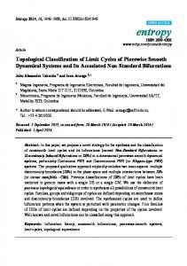
(e) Simple Cycle versus Non-Cyclic A Simple Cycle is a Simple Structure with at least one state that cycles with a period equal to its recurrence time. For two-state series the period is estimated by the sum of the median bout and the median pause duration. Medians are chosen rather than means, because observations in the rather long tails of these distributions tend to distort the mean. For example, in Table 4 the mean Active Sleep bout is 33.0 min, whereas the median is 42.5 min, largely because of the two extremely short 8- and lO-min bouts. The sum of the medians is used instead of the median recurrence time, since there is frequently one more bout or pause than there are recurrence times. In Table 4, for example, there are five recurrence times, but six Active Sleep bouts. When sample sizes are so small, it is important to use all available data. The estimate of period (a) is rounded to the nearest multiple of the sampling interval (in Table 4, 69.5 is rounded to 70 min, so d = 70) and the expected number of full cycles (C) is calculated. This number is the largest integer less than or equal to the number of observations, divided by the estimated period (in Table 4, 325170 = 4.6, so C = 4). As mentioned above, at least four full recurrences are required for analysis. The observations in the series are then arranged as a Raster Plot with the width equal to the estimated period. This is a matrix, the first row containing the first d observations, the second row containing the next d observations, and so forth. This format graphically presents the state cycles and facilitates their analysis. Figure 1 shows a Raster Plot of the sleep state series presented in Table 4. If this series were a Pure Cycle of period 70 min, the observations in each column would be identical; i.e., the proportion of pairwise agreements for the presence of the state within a column would be 1.0. On the other hand, if the state series were random, the agreement between pairs of observations within the same column would be the same as the agreement between any randomly selected observations. The kappa coefficient (K) is a statistic that measures such agreement, although it has not been used in this context before (20-22). It is expressed as: K = (P - Q)/(l - Q) where P is the proportion of pairs in the same column which are in agreement and Q is the overall proportion of pairs in agreement. The kappa coefficient is zero for a Random States Series and increases to 1.0 for a Pure Cycle. In more mathematical terms, d

K

= 1

2: j=1

Sleep, Vol. 7, No.1, 1984

Pi! - P)/(dp[1 - p])

11

THE DETECTION OF BEHA VIORAL STATE CYCLES t

1

2

(minutes)

3

4

567

.... I.... o.... I.... o.... I.... o.... 1.... o.... I.... o.... I.... o.... I.... 0

--

........................... . ............................ .

*************************

FIG.1. A raster plot of the sleep state series presented in Table 4 . • not observed. Period (d) = 70 min. Number of cycles (C) = 4.

*=

=

Active Sleep; •

=

Quiet Sleep;

where Pj is the proportion of the observations in columnj in which the state is present, and p, as before, is the overall proportion of observations in which the state is present. Since ~ P/l - P)ld is a measure of the within-column variance of the dichotomous obserVations and p(l - p) is a measure of overall variance, K measures the proportion of total variance accounted for by a Simple Cycle of length l1. The statistic K functions in a manner similar to spectral power in spectral analysis. The kappa coefficient is also an intraclass correlation coefficient (23), and so is comparable to the maximum autocorrelation coefficient in quantitative time series analysis. Both the Globus and Sackett procedures are based on measures similar to these. To demonstrate that a two-state series meets the criteria for a Simple Cycle, kappa must be significantly greater than zero. For a Random States null hypothesis, approximately -

K

SK

~

n(O 1) '

where

~[l

SK2

T

- 4p(l - P)(l _ td) + 2td(l _ td)] p(l - p)

T

T

T'

TABLE 4. A Simple Cycle sleep record Active

Quiet

8 25 46 27 41 28 49

General statistics: Duration (D = 325 min Sampling Interval = 1 min Proportion Active Sleep (P) = 0.61 Median Active Bout = 42.5 min Median Quiet Bout = 27.0 min Recurrence Time = 70 min

17 44 30 10

Complex Structure: Z (active) = 0.39 (ns, 6 bouts) Z (quiet) = 0.00 (ns, 5 bouts) Simple Cycle: K = 0.78 Z = 20.0 (p < 0.01)

Sleep, Vol. 7, No.1, 1984

H. C. KRAEMER ET AL.

12

Thble 4 illustrates the manner in which these procedures are applied serially to the sleep of a normal 8-week-old infant. There is no evidence for Complex Structure (Z = 0.39 and Z = 0.00, but there are fewer then eight bouts for each series). The kappa coefficient, however, is 0.78 (ZK = 20.0, p < 0.00. This significant kappa suggests a Simple Cycle of 70 min, comprising an Active Sleep duration of about 43 min and a Quiet Sleep duration of 27 min. Figure 1 is the Raster Plot of this child's data, and visually confirms the presence of a strong Simple Cycle. (d) Organized Transitions versus Random Transitions Series Non-cyclic two-state series are always alternating bouts of the two states. If there are more than two states, a non-cyclic multiple-state series mayor may not display organized transitions between the states (cf. Table 1, a). To demonstrate organization at this level, one estimates the expected proportions of state-to-state transitions when transitions are random. These proportions are

%=

(no. transitions to J)

+ (no. transitions from j)

2(total no. of transitions)

where j is any of the possible states. The expected number for each possible transition in the random case is then E· = lJ

o·/.

1 - qi

i#-j

where 0i. is the number of transitions out of state i. We use Oij to represent the number of observed transitions from state i to state j, and Eij to represent the expected number of transitions from state ito statej. We define Eii = 0 for all i. Under the null hypothesis of random transitions the test statistic [sum of (observed - expected)2/expected] is

x2

=

2: (Oi)

- Ei)?/Ei}

i""J

This statistic, X2 , has a chi-squared distribution with (M - 1)2/2 degrees of freedom. If this test is to be used, no more than 20% of the expected values (Eij) may be less than 5 and none may be less than 1 (24). If the test proves significant, the distinction between one-step versus multiple-step semi-Markov chains may be pursued (cf. 9). Thble 5 presents the nighttime state series of a 20-week-old infant, including Awake as well as Active and Quiet Sleep. The calculations described above are detailed in Table 5. Here, X2 = 9.26 (p < 0.05); but despite the relatively large number of transitions (38), the expected values do not meet the minimum criteria for valid testing; 33% of expected values (2/6) are less than 5. The transitions do show a pattern typical of younger infants: there are no direct transitions between Quiet Sleep and Awake. The bout series for Active Sleep in Table 5 has a significant Turning Points test (Z = - 2.47, p < 0.05). Thus this series is classified as a Complex Structure. If the

Sleep, Vol. 7, No.1, 1984

r

TABLE 5. An Organized Transitions sleep record Awake

Active

11 39 16 24 25 6 3 11 43 46 12 II

,

I

From QS From AS From AW

5

=

38 To AS

To AW

x 11 0

11 x 8

0 8 x

To QS

To AS

To AW

Expected:

7 18 7 From QS From AS From AW

26 20

x 11.0 2.9

7.7 x 5.1

3.3 8.0 x

35 31 8 21 13

X2 = 9.26, df = 2 But two cells (33%) are