The Development of Nearly Deterministic Methods for

The Development of Nearly Deterministic Methods for Optimising Protein Geometry Dem Department Informatik der Fakult¨at f¨ ur Mathematik, Informatik und Naturwissenschaften an der Universit¨ at Hamburg eingereichte Dissertation zur Erlangung des akademischen Grades DOCTOR RERUM NATURALIUM (Dr. rer. nat.) in der Abteilung Biomolekulare Modellierung des Zentrums f¨ ur Bioinformatik Hamburg

vorgelegt von Dipl.-Bioinf. Gundolf Walter Hubert Schenk geboren am 3.2.1979 in Hannover

Hamburg, 27. Oktober 2011

Tag der m¨ undlichen Pr¨ ufung: Erstgutachter: Zweitgutachter:

28. M¨arz 2012 Herr Prof. Dr. Andrew Torda Herr Prof. Dr. Jianwei Zhang

Zusammenfassung Proteine sind langkettige Biomolek¨ ule mit charakteristischen Funktionen, die eine Hauptrolle in allen Lebewesen einnehmen. Diese Funktion ergibt sich aus der Proteinstruktur, die wiederum durch einen komplizierten Mechanismus basierend auf der Aminos¨auresequenz bestimmt wird. Der genaue Vorgang ist nicht vollst¨andig verstanden, aber die Strukturen zu kennen ist wichtig f¨ ur die pharmazeutische Industrie, sowie f¨ ur die Bio- und Nanotechnologie. Leider ist es langsam und teuer sie experimentell zu bestimmen. Hohes Interesse besteht auch daran die Sequenz anzupassen um stabile industrielle Enzyme zu machen oder um Molek¨ ule mit speziellen Formen herzustellen, z.B. f¨ ur Biosensoren. Eine Struktur am Computer anhand der Sequenz vorherzusagen ist ein klassisches Problem der theoretischen Biochemie, welches bisher nicht gel¨ost wurde. In dieser Arbeit liegt der Schwerpunkt auf methodologischen Verbesserungen, die verbreitete chemische Annahmen vermeiden. Eine allgemeine Methode zur Erstellung numerischer Modelle wird hier entwickelt und analysiert. Sie basiert auf einem statistischen Korrelationsmodell von Sequenz und Struktur und benutzt Ideen aus der selbst-konsistenten Mittelfeld (SCMF) Optimierung. Das Verfahren l¨asst sich erfolgreich auf die Strukturvorhersage- und Sequenzdesignprobleme anwenden ohne eine Boltzmann Statistik anzunehmen. Das statistische Modell basiert auf einer Mischverteilung von bivariaten Gaußverteilungen und 20-wege Bernoulliverteilungen. Die Gaußverteilungen modellieren die kontinuierlichen Variablen der Proteinstruktur (Torsionswinkel) und die Bernoulliverteilungen erfassen die Sequenzpr¨aferenzen. Anstelle ein Protein als statistische Einheit zu verstehen, werden hier leichter zu verarbeitende Fragmente betrachtet. Mehrere Ans¨atze sie wieder zusammenzusetzen werden diskutiert. Aber die Fragmente bilden lokale statistische Einheiten, die nicht notwendiger Weise miteinander u ¨bereinstimmen. Ein passendes Verfahren solche Inkonsistenzen zu behandeln, ist die SCMF Optimierung. Mittelfeld oder SCMF Verfahren betrachten das zu optimierende System in allen L¨osungszust¨anden gleichzeitig. In bestehenden Ans¨atzen wurde dazu ein Energiepotential erstellt, das gemittelte, paarweise Wechselwirkungen zwischen Untersystemen abbildet. Die Zustandsgewichte der Untersysteme wurden durch wiederholte Anwendung des Boltzmannverh¨altnisses alternierend in Energien und Wahrscheinlichkeiten umgerechnet bis ein selbst-konsistenter Zustand des gesamten Systems erreicht wird. Mit dem hier pr¨asentierten Ansatz ist es m¨oglich die Zustandswahrscheinlichkeiten direkt zu optimieren. Die Boltzmannverteilung ist keine notwendige Annahme. Daher ist die Methode auch auf Systeme mit unbekanntem Ensemble anwendbar.

Abstract Proteins are long-chained biomolecules with distinctive functions, that take a major role in all living systems. The function is defined by the protein structure, which in turn is determined via a complicated mechanism based on the amino acid sequence. The exact procedure is not fully understood. However, knowing the structure is important for the pharmaceutical industry as well as bioengineering and nanotechnology. Unfortunately, determining it experimentally is slow and expensive. There is also much interest in being able to adapt the sequence to make stable industrial enzymes or to form molecules with specialised shapes, e.g. for biosensors. Predicting a structure computationally from the sequence is a classic problem in theoretical biochemistry, that has not been solved yet. In this work the emphasis lies in methodological improvements, that avoid common chemical preconceptions. A general method for building numerical models is developed and analysed here. It is based on a statistical correlation scheme of sequence and structure using ideas from self-consistent mean field (SCMF) optimisation. The procedure is successfully applied to the structure prediction and sequence design problems without using a Boltzmann formalism. The statistical model is based on a mixture distribution of bivariate Gaussian and 20-way Bernoulli distributions. The Gaussian distributions model the continuous variables of the structure (dihedral angles) and the Bernoulli distributions capture the sequence propensities. Instead of treating the protein as a statistical unit, easier to handle fragments are used. Several approaches to recombine them are discussed. But the fragments form local statistical units that do not necessarily agree with each other. A method suited to deal with such inconsistencies is SCMF optimisation. Mean field or SCMF methods optimise a system by treating all solution states at the same time. In existing approaches, an energy potential was introduced that reflects the pairwise mean interaction between subsystems. The state weights of the subsystems were converted alternately into energies and probabilities by applying the Boltzmann relation repeatedly until a self-consistent state for the whole system is reached. With the approach presented here it is possible to optimise the state probabilities directly. The Boltzmann distribution is essentially an unnecessary assumption. Therefore, the method is also applicable to systems with an unknown ensemble.

Contents 1 Introduction 1.1 Proteins . . . . . . . . . . . . . . . 1.2 Protein Classification . . . . . . . . 1.2.1 Protein Descriptors . . . . . 1.2.2 Classifications . . . . . . . . 1.2.3 Protein Structure Prediction 1.2.4 Protein Sequence Prediction 1.3 Bayesian Classification of Proteins . 1.3.1 Protein Descriptors . . . . . 1.3.2 Class Models . . . . . . . .

. . . . . . . . .

. . . . . . . . .

. . . . . . . . .

. . . . . . . . .

. . . . . . . . .

. . . . . . . . .

. . . . . . . . .

. . . . . . . . .

. . . . . . . . .

. . . . . . . . .

. . . . . . . . .

. . . . . . . . .

1 1 2 2 3 4 5 5 5 7

2 Protein Reconstruction 2.1 Probability Model . . . . . . . . . . . . . . . . 2.1.1 Dihedral Angles . . . . . . . . . . . . . 2.2 Methods . . . . . . . . . . . . . . . . . . . . . 2.2.1 Dihedral Angles . . . . . . . . . . . . . 2.2.2 Backbone Reconstruction . . . . . . . 2.2.3 Amino Acids . . . . . . . . . . . . . . 2.3 Results . . . . . . . . . . . . . . . . . . . . . . 2.3.1 Influence of Bond Lengths and Angles 2.3.2 Dihedral Angle Reconstruction . . . . 2.3.3 Sequence Reconstruction . . . . . . . . 2.4 Discussion . . . . . . . . . . . . . . . . . . . . 2.4.1 Influence of Bond Lengths and Angles 2.4.2 Dihedral Angle Reconstruction . . . . 2.4.3 Sequence Reconstruction . . . . . . . .

. . . . . . . . . . . . . .

. . . . . . . . . . . . . .

. . . . . . . . . . . . . .

. . . . . . . . . . . . . .

. . . . . . . . . . . . . .

. . . . . . . . . . . . . .

. . . . . . . . . . . . . .

. . . . . . . . . . . . . .

. . . . . . . . . . . . . .

. . . . . . . . . . . . . .

. . . . . . . . . . . . . .

11 11 12 19 20 25 26 28 29 29 32 34 34 35 36

3 Self-consistent mean field optimisation 3.1 Standard SCMF . . . . . . . . . . . . . . . . . . . . . . . . . . . . 3.2 Purely statistical SCMF . . . . . . . . . . . . . . . . . . . . . . . 3.3 Simulated Annealing . . . . . . . . . . . . . . . . . . . . . . . . .

39 40 41 43

i

. . . . . . . . .

. . . . . . . . .

. . . . . . . . .

. . . . . . . . .

. . . . . . . . .

4 Structure Prediction 4.1 Methods . . . . . . . . . . . . . . . . . . . . 4.1.1 Optimising Class Weights . . . . . . 4.1.2 Calculating and Sampling Structures 4.1.3 Refining Structures . . . . . . . . . . 4.1.4 CASP . . . . . . . . . . . . . . . . . 4.2 Results . . . . . . . . . . . . . . . . . . . . . 4.2.1 Most Likely Structures . . . . . . . . 4.2.2 Sampling . . . . . . . . . . . . . . . 4.2.3 Optimising Class Weights . . . . . . 4.2.4 Scoring . . . . . . . . . . . . . . . . . 4.2.5 CASP . . . . . . . . . . . . . . . . . 4.3 Discussion . . . . . . . . . . . . . . . . . . . 4.4 Outlook . . . . . . . . . . . . . . . . . . . . 4.4.1 Sequence Profiles . . . . . . . . . . . 4.4.2 Loop Modelling . . . . . . . . . . . . 5 Sequence Prediction 5.1 Methods . . . . . . . . . . . . . . . . . . 5.1.1 Optimising Residue Probabilities 5.1.2 Generating Sequences . . . . . . . 5.2 Results . . . . . . . . . . . . . . . . . . . 5.2.1 Optimising Residue Probabilities 5.2.2 Generating Sequences . . . . . . . 5.3 Discussion . . . . . . . . . . . . . . . . .

. . . . . . .

. . . . . . .

. . . . . . . . . . . . . . . . . . . . . .

. . . . . . . . . . . . . . . . . . . . . .

. . . . . . . . . . . . . . . . . . . . . .

. . . . . . . . . . . . . . . . . . . . . .

. . . . . . . . . . . . . . . . . . . . . .

. . . . . . . . . . . . . . . . . . . . . .

. . . . . . . . . . . . . . . . . . . . . .

. . . . . . . . . . . . . . . . . . . . . .

. . . . . . . . . . . . . . . . . . . . . .

. . . . . . . . . . . . . . . . . . . . . .

. . . . . . . . . . . . . . . . . . . . . .

. . . . . . . . . . . . . . .

47 49 49 51 54 56 57 57 58 62 64 66 70 73 73 74

. . . . . . .

77 78 79 80 80 81 82 84

6 Conclusions and Outlook

87

A Directional Statistics A.1 Means and Differences . . . . . . . . . . . . . . . . . . . . . . . . A.2 Circular Distributions . . . . . . . . . . . . . . . . . . . . . . . .

93 93 94

B Analytic Derivation of the Adaptive Cooling Threshold

99

Bibliography

103

Curriculum Vitae

111

Publications

112

Acknowledgements

113

ii

Chapter 1 Introduction Modelling protein molecules means trying to predict their structure given their amino acid sequence. The problem has been in the literature since the first protein structures were solved [KDS+ 60, PRC+ 60], but remains a challenging task. Finding models for protein structures experimentally is a rather costly challenge. So since the beginnings the computational modelling has been a helpful crucial tool. Only in recent years has there been much success in this area, although still there are many open questions and without experimental techniques no reliable model can be obtained [OBH+ 99, BDNBP+ 09, CKF+ 09, MFK+ ]. However, with the initiatives for structural genomics the number of experimentally solved models is increasing rapidly. The growing database of solved protein structures offers new ways to model proteins on a statistical basis. In this work, an innovative optimisation scheme based on a purely statistical protein model is developed from ideas of self-consistent mean field optimisation. With a rather simple scoring scheme we give a proof-of-principle and show how to apply our approach to structure prediction and sequence design.

1.1

Proteins

Proteins are biomolecular polymers [RR07], i.e. they are built as chains or sequences of 20 different amino acid types connected via peptide bonds found, for example, in biological cells. The chain of atoms directly involved in the peptide bond is called the backbone and the other atoms are called sidechains. Figure 1.1.1 sketches a small stretch of such a polymer. The typical lengths of protein sequences are between 50 and 800 amino acids long. In solution, e.g. in the cell, they fold to a three-dimensional structure. That means, the atoms of a protein arrange in space in a more or less compact way and this arrangement stays mostly the same throughout the protein’s lifetime though sometimes flex1

R

O amino (N) terminus

ψ

Cα

C

α

C ω N φψ

carboxyl (C) terminus

φψ

φψ

φ

H Figure 1.1.1: The backbone of a protein is connected via peptide bonds. The sidechains are only symbolised by the purple dots.

ibility has been observed. The determination of this structure is mainly driven by the polymer’s amino acid composition, i.e. its sequence, and sometimes helper molecules, such as chaperones and other cofactors [Anf73, MH93, vdBWDE00]. In the biological context each protein is specialised in a distinct biochemical function, for example in a metabolic process. This function is solely determined by the proteins structure, i.e. by the positions of all protein atoms in space. Therefore, the knowledge of the protein structure is crucial in understanding its function and role in the biochemical processes that drive life. Many experimental methods are used to solve the structure of a protein. The most important ones are probably X-ray crystallography, nuclear magnetic resonance spectroscopy and electron microscopy. Structures determined via X-ray crystallography typically have the highest resolution allowing the most detailed view on the atom positions. Almost all solved structures are deposited in the Protein Data Bank [PDBa, BWF+ 00], currently (2011-07-18) consisting of 72000 entries of which 64000 are determined by X-ray crystallography. If a protein structure is known, one can display it via 3D rendering techniques on a computer screen. Figure 1.1.2 shows several representations and levels of abstraction that can be chosen in such programs [PGH+ 04]. The colouring is according to secondary structure, that is, local regular structure of the backbone, e.g. α-helices in red or β-strands in purple.

1.2 1.2.1

Protein Classification Protein Descriptors

Monomer proteins may be described by three levels, primary structure, secondary structure and tertiary structure. The primary structure is the sequence of amino 2

(a) all atom sphere

(b) all atom ball & stick

(c) backbone chain trace

(d) backbone ribbon

Figure 1.1.2: Representations and levels of abstraction for a small protein structure (pdb-id: 1CTF). Pictures are made by UCSF Chimera [PGH+ 04].

acid types, i.e. a text string. By secondary structure the sequence of local consecutive structural subunits is denoted, mostly also a character string. Tertiary structure is the three-dimensional arrangement or the spatial coordinates of the polymer, typically a table of atom positions. In this thesis, the primary structure will be called “sequence” and the tertiary structure “structure” or “fold”. The backbone of a protein can be described solely by the sequence of dihedral angles at the α-carbons as the amide plane is known to form a rigid unit, figures 1.1.1 and 1.3.1. The sidechains are often only described by their type and are modelled separately. Figure 1.2.1 shows the histogram of the dihedral angles φ and ψ in the protein data bank [PDBa].

1.2.2

Classifications

Typically classifications are used to simplify the handling of proteins. Their scope is either to provide an easy, human-interpretable way for distinguishing between proteins or to enable computers to perform calculations such as comparisons and predictions in reasonable time. That means, a classification basically reduces the complexity of the task and often leads to an approximation. For a review of structural and functional protein classifications, see [OCE+ 03]. We have developed and successfully applied a scoring scheme to protein comparisons using sequence, structure or both [SMT08b, MST09]. It is based purely on Bayesian statistics and derived via a maximally parsimonious automatic classifier [CPT02, CS96] from overlapping protein fragments. In this work we use this classification for the sake of optimisation and prediction of unknown features, such as structure or sequence. 3

≥ 0.001

π

frequency

ψ

π 2

0

− π2 −π

−π

− π2

π 2

0 φ

π

≤ 0.0001

Figure 1.2.1: Distribution of the dihedral angles φ and ψ in the protein database.

1.2.3

Protein Structure Prediction

Structure prediction means to propose one or more structures that a given sequence would adopt in a living cell. There are two broad categories of such programs: 1. homology based and 2. ab initio. In homology-based modelling one uses structural information from known templates. Programs based on this idea perform very well if homologous templates can be identified. The quality of the outcome is highly dependent on the quality and identification of a related template. Finding such a template can be a difficult task, which often gives no satisfying results. If that is the case, the ab initio modelling programs try to predict the structure from scratch without explicitly knowing any related structures. This approach is less reliable than homology modelling for the cases where the structure of a related protein is known, but they are the only applicable method when no template structure is available. Given that homology-based and ab initio methods work best on different problems, some automatic methods attempt to select or combine the approaches. In the CASP 8 meeting the Robetta and the Zhang servers were among the top candidates [BDNBP+ 09, CKF+ 09]. These two programs are difficult to put into one of the described categories. They are fragment based, i.e. the amino acid sequence 4

is split into short fragments and these fragments are used as queries on the template database. By doing that, the advantage of the homology-based approaches are also available for sequences where no complete structural template could be found. However still, if no or only bad template fragments can be found, modelling from scratch becomes necessary. In this work we propose a new approach, which is based on self-consistent mean-field optimisation (SCMF), but using a framework of descriptive statistics and simulated annealing (see section 1.3 and chapter 3).

1.2.4

Protein Sequence Prediction

Sequence prediction, or more often sequence optimisation, is the task of finding one or more amino acid sequences that fold to a given structure. It can be viewed as the inverse problem to structure prediction. This NP-hard problem [PW02] is not only fundamentally interesting but also relevant for understanding the relation between sequence and structure. It is likely to be of practical use for improving protein stability, for example thermostability in washing powder, for specialising reaction conditions in the production of biodiesel or even for nanotechnology, for example in the case of personalised medicine. Therefore, this problem is often called protein design. Despite some impressive literature results, the design steps have often been rather ad hoc and the method is far from routine [KB00, KAS+ 09, FF07, SJ09, KAV05, JAC+ 08, SDB+ 08, Tor04]. In this work we propose an innovative general approach, which is based on the same ideas as structure prediction, i.e. self-consistent mean-field optimisation (SCMF) on a framework of descriptive statistics and simulated annealing (see section 1.3 and chapter 3).

1.3

Bayesian Classification of Proteins

The classification used in this work has been described earlier [SMT08b]. However, the main ideas are explained also here.

1.3.1

Protein Descriptors

The focus of this work is on the conformation of the protein backbone. That means, the modelling of the side-chain conformations is postponed. This is a typical procedure and simplifies the problem. The proteins are described in terms of amino acid sequence and dihedral backbone angles. Here, the variability of bond lengths and bond angles in the backbone 5

O

R

trans peptide group 1.24˚ A

120.5◦

1. 5

Cα

1˚A

C

123.5◦

1. 3

✁ ✁ peptide bond✁

122◦

3A ˚

116◦

119.5◦

N

1. 4

A 6˚

111◦

118.5◦ PP P

A 1.0˚

Cα

P amide plane

H Figure 1.3.1: Standard geometry in a trans peptide group. (the amide plane) within and across proteins is assumed very low and is therefore ignored, see figure 1.3.1. The carbonyl group and the amide group are nearly in the same plane and this unit (light blue) is very rigid [HBA+ 07]. For its actual influence on the full backbone (re)construction see subsection 2.3.1. For a protein consisting of l amino acids, i.e. of chain length l, 2l − 2 dihedral angles describe the conformation of the backbone, namely l − 1 φ and l − 1 ψ angles (see figure 1.1.1). In this work a Bayesian classification is used to model the statistical properties [SMT08b], see also subsection 1.3.2.

1.3.1.1

Overlapping Fragments

At the heart of the method is a classification of protein fragments. A protein is then represented as the set of all possible overlapping fragments, given by  (si , xi )

 si = (ai , . . . , ai+k−1 )T ∀i ∈ [1, l − k + 1] , ∧ xi = (φi , ψi , . . . , φi+k−1 , ψi+k−1 )T

where ai ∈ [1, 20] is the amino acid type at residue i. The non-existent dihedral angles φ1 and ψl are ignored and T denotes the transpose. 6

1.3.1.2

Dihedral Angles, Bond Lengths and Angles

The typical distances and angles on the amide plane are shown in figure 1.3.1. As these values are fixed the backbone conformation is solely described by its dihedral angles, φ and ψ (see also figure 1.1.1). When dealing with angles, one has to be aware of the specialities characterising angles, see appendix A. The classification in use is based on Gaussian (normal) distributions and has no knowledge about the periodic nature of angles. It is therefore important to choose boundaries covering one period (no redundancy) with minimal border effects. That means, the boundaries  π 3πare
shifted to low populated areas. For φ this is [0, 2π) and for ψ this is − 2 , 2 . Figure 1.3.2 shows a scatterplot of the angles pairs found in the protein database [PDBa].

1.3.2

Class Models

The class models used for the amino acid labels are multiway Bernoulli distributions pCj (S = si ) and for angles a multivariate Gauss distribution pCj (X = xi ). These are chosen mainly for convenience so that the AutoClass-C package [CPT02, CS96] could be used for the parameter search. The combination of these models is a classical mixture model: n X p((S, X) = (si , xi )) = wj pCj (S = si ) pCj (X = xi ),

(1.3.1)

j=1

where wj denotes the weight for the class Cj and n is the number of classes. The class weights may also be interpreted as prior probabilities of the fragment F = (S, X) being in class Cj , which is then denoted by p(F ∼ Cj ) = wj . Formula (1.3.1) comprises two parts, the multiway Bernoulli distributions and the multivariate Gauss distribution. These are explained in the next two paragraphs. 1.3.2.1

Multiway Bernoulli Distribution

The amino acid labels are modelled by several classes of multiway Bernoulli distributions. In each class model the dependencies between residues are completely ignored. That means, a sequence fragment si ∈ [1, 20]k is interpreted as an instance of a discrete random vector S of k independent random variables St with possible outcomes in [1, 20] each. In each dimension each amino acid label is assigned the conditional probability of observing this label given the class model Cj , i.e. pCj (S = si ) =

k Y t=1

pCj (St = sit ).

(1.3.2) 7

3π

2π

ψ

π

0

−π

−2π −2π

−π

0

π

2π

3π

4π

φ

Figure 1.3.2:

Periodic Ramachandran plot: red box shows the original ranges, [−π, π) × [−π, π); blue box shows the shifted borders to underpopulated areas, [0, 2π) ×  π 3π
−2, 2 .

8

However, in the weighted sum of all classes, formula (1.3.1), the residues are effectively correlated. 1.3.2.2

Multivariate Normal Distribution

The structural terms, i.e. the dihedral angles, are modelled by several classes of multivariate Gaussian or normal distributions. In each class model a fragment of dihedral angles is interpreted as an instance of a continuous random vector X of 2k correlated random variables. The model allows the full correlation between the dihedral angles, but, to
keep computational costs low and avoid overfitting, only angle pairs xit = ψφtt are allowed to correlate. However, as in the case of the Bernoulli distributions, the mixture model (formula (1.3.1)) captures the full correlation. Each fragment xi is assigned the conditional probability density of observing the dihedral angles given the class model Cj , i.e. h
T i
exp − 12 xi − µj C −1 x − µ i j j p pCj (X = xi ) = (2π)2k | det C j | ≈

k Y t=1

pCj (X t = xit )

h
T i
−1 k exp − 1 x − µ x − µ C Y it it j jt jt t,t 2 q , = 2 | det C (2π) | t=1 j t,t

where µj =


T µj T1 , . . . , µj Tt , . . . , µj Tk

  and C j = C j t,t′

t,t′ ∈[1,k]

with µj t =



µj t φ µj t ψ



cj tφ ,t′ φ cj tφ ,t′ ψ cj tψ,t′ φ cj tψ,t′ ψ

with C j t,t′ =

is the vector of means ! is the 2k × 2k cov-

ariance matrix of class Cj . In the next chapter the statistical model is analysed extensively and several formal approaches for reconstructing dihedral angles and amino acids from it are developed. Chapter 3 introduces the innovative optimisation method. And in chapters 4 and 5 the methods are applied to structure prediction and sequence design, respectively. Finally, in chapter 6 conclusions and outlook are given.

9

10

Chapter 2 Protein Reconstruction In this chapter the predictive potential of the statistical descriptor based on the Bayesian classification is analysed in order to see how well the full protein description is approximated. Therefore, the full description is reconstructed from the statistical classification and checked against the original description. Before the reconstruction approaches are introduced in section 2.2, it is important to have a thorough understanding of the probability model. Therefore, the statistical descriptors are introduced formally along with some explanations about their theoretical properties in the next section.

2.1

Probability Model

As has been explained previously [SMT08b], the classification can be used to  describe a protein by a set of class probability vectors v i i ∈ [1, l − k + 1] constructed from overlapping fragments. First the backbone of the protein is broken into maximally overlapping fragments by sliding a window of length k. Each fragment is described by its dihedral angles (or amino acid labels), from which probability vectors are calculated. The vector elements are then associated with the Gaussian terms (Bernoulli terms) in different ways, e.g. to build mixture distributions (subsection 1.3.2) or to estimate continuous and discrete features (subsections 2.2.1 and 2.2.3). Here, the theoretical properties of the model are explained for reconstructing continuous features (i.e. dihedral angles), as their handling is more complicated than the discrete features (amino acid labels) and many insights apply for both cases. 11

2.1.1

Dihedral Angles

According to [SMT08b, CS96] the elements of the probability vector v i = vij T

for a structure fragment xi = (φi , ψi , . . . , φi+k−1 , ψi+k−1 ) are given by wj pCj (X ≈ xi )
vi j = pxi (F ∼ Cj ) = p F ∼ Cj X ≈ xi = P n wj ′ pCj′ (X ≈ xi )




j∈[1,n]

(2.1.1)

j ′ =1

and can be interpreted as the n-dimensional vector of probabilities of all n classes Cj given the dihedral angles xi . The prior class weights wj directly come from the classification and the structural class weights (joint probabilities) are taken to be Z Z (2.1.2) pCj (X ≈ xi ) = · · · pCj (X = x) dx1 . . . dx2k , A

where A = [xi 1 − ǫ1 , xi 1 + ǫ1 ] × · · · × [xi 2k − ǫ2k , xi 2k + ǫ2k ] is the integration domain 2k with ǫ ∈ R+ being some small vector-valued error. From first principles one might be tempted to estimate the original angles of the fragment by the expectation values of the associated mixture distribution (formula (1.3.1), page 7) [Kre98]. The vector of expectation values using the probability vector corresponding to the fragment is given by Z Z X n est vij pCj (X = x) dx1 . . . dx2k xi = ··· x =

R2k n X

vi j

j=1

=

n X

j=1

Z

···

R2k

Z

x pCj (X = x) dx1 . . . dx2k

vi j µ j ,

(2.1.3)

j=1

where µj is the vector-valued mean of the multivariate Gaussian modelling the class Cj . 2.1.1.1

Limitations of Joint Probabilities

The formula for expectation values (2.1.3) has some principal limitations when used with random vectors. First principles say, the expectation value of a random vector is defined component-wise [Kre98]. Formula (2.1.3) can be viewed as an average of the class means, which does not lead to the right answer as the 12

Figure 2.1.1: The ellipsoidal contours of two bivariate classes (red and blue). The angle pair to be estimated is marked by a circle.

probability vectors (formula (2.1.1)) comprise joint probabilities for multivariate classes. Let us consider the origin of these probabilities in order to understand why this a problem. For each class the probability densities of the Gaussian distribution functions define contours in the conformational space (i.e. the space of dihedral angles) in shape of ellipsoids. In the ideal case, these ellipsoids would intersect in a single point, which would be the original angles corresponding to the probability vector. However, a weighted average of two class means would lie only somewhere on a line connecting the centres of the classes. For two dimensions this problem is illustrated in figure 2.1.1 and is described formally in the following. Let Aj = C −1 j be the inverse correlation matrix of class Cj , then the probability density for two correlated angles θ1 and θ2 is given by    exp − 1 θ − µ , θ − µ
A j 1 j1 2 j2 2 θ1 p = p Cj θ2 (2π)2 | det C j |

θ1 −µj 1 θ2 −µj 2




.

This is equivalent to

 q  θ1 (2π)2 | det C j | −2 log pCj θ2  
θ1 − µ j 1 = θ1 − µ j 1 , θ2 − µ j 2 A j θ2 − µ j 2 2 2 XX

= aj t,t′ θt − µj t θt′ − µj t′ . 

t=1 t′ =1

13

(2.1.4)

The expression (2.1.4) is the equation for the ellipsoidal contour, also known as the Mahalanobis distance [Mah36]. Averaging class means with one single weight per class will not lead to the original angles in general. With joint probabilities of whole fragments, it is impossible to find a correct weighting, as illustrated in figure 2.1.1. Instead, the use of marginal probability densities to average the class means correctly with weights for each dimension is considered and analysed in the following

2.1.1.2

Marginal Probability Density Vectors

Marginal probability density vectors are defined in close analogy to normal probability vectors. A third index t ∈ [1, k] reflecting the position in the fragment is added to the known indices for fragments i ∈ [1, l − k + 1] and for classes j ∈ [1, n]. For the dihedral angle pair xi t = (xi tφ , xi tψ )T = (φi+t−1 , ψi+t−1 )T at the tth residue of a fragment xi of length k the elements
of the marginal marg marg are taken to be probability density vectors v marg = v marg i i,1 , . . . , v i,t , . . . , v i,k v marg i,t

T    marg v   i,tφ j =   marg j∈[1,n]  vi,tψ j

j∈[1,n]

!T

p F ∼ Cj Xtφ = φi+t−1 j∈[1,n]

= p F ∼ Cj Xtψ = ψi+t−1 j∈[1,n]  T         =      

 wj pCj (Xt φ = φi+t−1 )    n  P wj ′ pCj′ (Xtφ = φi+t−1 ) ′  j =1 j∈[1,n]  wj pCj (Xtψ = ψi+t−1 )    n P  wj ′ pCj′ (Xt ψ = ψi+t−1 ) j ′ =1

j∈[1,n]

       .     

(2.1.5)

Actually, each v marg is a probability density matrix consisting of 2k columns i and n rows. The marginal probability density functions pCj (Xtφ = φi+t−1 ) and pCj (Xtψ = ψi+t−1 ) are univariate Gaussian distributions with parameters µj tφ , cj tφ ,tφ and µj tψ , cj tψ,tψ , respectively [Pol95]. With these marginal probability vectors the expectation values can be formulated 14

est in analogy to equation (2.1.3) for xi est tφ and xi tψ , respectively, by

xi est tφ

=

=

= ∧ xi est tψ =

Z

φ

n X

marg vi,t pCj (Xt φ = φ) dφ φ

j j=1 R Z n X marg φ pCj (Xtφ vi,tφ j j=1 R n X marg vi,tφ µj tφ j j=1 n X marg vi,t µ . ψ j j tψ j=1

= φ) dφ

(2.1.6φ ) (2.1.6ψ )

The marginal probabilities used here, allow one to calculate expectation values in accordance with first principles by averaging class means component-wise. Still, this will not necessarily lead to the original angle values as the Gaussian probability densities do not scale linearly in the space between the class means. They rather lie on some manifold where linear Euclidean distances are not valid. The observations in paragraph 2.1.1.1 show that the manifold is defined by the Mahalanobis distance (formula (2.1.4)). However, in order to use a linear average of class means, the weights must scale linear with the angle value that led to the class weights. In the next paragraph a linearisation of this manifold is derived for the class weights. 2.1.1.3

Linearisation of Class weights

In this paragraph, weights for averaging mean values of univariate Gaussian distributions are derived step by step. Consider the simple case of two mean values µ1 and µ2 . Given two density values p1 , p2 from two univariate Gaussians with parameters µ1 , σ12 and µ2 , σ22 , respectively, and assuming that p1 and p2 were derived from a single value α, then this value can be estimated by averaging over the class means µ1 6= µ2 using suitable weights w1 and w2 , i.e. αest = w1 µ1 + w2 µ2 with 1 = w1 + w2 . As α is an angle, without loss of generality it can be assumed that µ1 ≤ α ≤ µ2 holds. Otherwise one µ is substituted with its periodic image, i.e. µ + 2π or µ − 2π, and exchanged with the other µ. In the following the unknown weights w1 , w2 are analytically derived. As αest is unknown, a formulation only based on the density values p1 and p2 is given below. 15

Proposition:

w1 ∧ w2

√

q √ 2σ1 = 1+ − log [ 2πσ1 ] − log [p1 ] µ1 − µ2 √ q √ 2σ2 = 1− − log [ 2πσ2 ] − log [p2 ] µ1 − µ2

Proof: Let α be the original angle. Then the densities p1 and p2 are by the definition of univariate Gaussian (normal) distribution functions taken to be

  1 (α − µ1 )2 p1 (α) = √ exp − 2σ12 2πσ1   1 (α − µ2 )2 ∧ p2 (α) = √ exp − . 2σ22 2πσ2

Substituting into the proposed equations for the weights gives

√

r

h√ i − log 2πσ1 − log [p1 (α)] v h i  u (α−µ1 )2 √ u h i exp − 2σ2 √ 2σ1 u 1  t− log 2πσ1 − log  √ = 1+ µ1 − µ2 2πσ1 s √ i (α − µ )2 i h√ h√ 2σ1 1 + log = 1+ − log 2πσ1 + 2πσ 1 µ1 − µ2 2σ12

2σ1 w1 (α) = 1 + µ1 − µ2

(α − µ1 ) µ1 − µ2 √ r h√ i 2σ2 ∧ w2 (α) = 1 − − log 2πσ2 − log [p2 (α)] µ1 − µ2 (α − µ2 ) . = 1− µ1 − µ2 = 1+

16

1

weight

0.8 0.6 0.4 0.2 0 -3

-2

-1

0

1

2

α p1

p2

w1

w2

Figure 2.1.2: Two Gaussians with parameters µ1 = −2, σ12 = 1 and µ2 = 1, σ22 = 2 and their

corresponding linearised weights.

In fact, the weights w1 (α), w2 (α) scale linear with α. It remains to be shown that α equals αest : αest = w1 µ1 + w2 µ2     (α − µ2 ) (α − µ1 ) µ1 + 1 − µ2 = 1+ µ1 − µ2 µ1 − µ2 (µ1 − µ2 )µ1 + (α − µ1 )µ1 + (µ1 − µ2 )µ2 − (α − µ2 )µ2 = µ1 − µ2 2 2 µ1 − µ2 µ1 + αµ1 − µ1 + µ1 µ2 − µ22 − αµ2 + µ22 = µ1 − µ2 αµ1 − αµ2 = µ1 − µ2 = α ✷ The weights and the two Gaussians are shown in figure 2.1.2. This can be generalised to n Gaussians by sorting them according to their means ′ and calculating the pairwise weights wj,j ′ ∀j, j ′ ∈ [1, n]. Let wj,j ′ be an auxiliary 17

variable taken to be  √ q √  2σj   − log [ 2πσj ] − log [pj ] if µj < µj ′ , 1 +   µj − µj ′   √ q ′ √ 2σj wj,j ′ = − log [ 2πσj ] − log [pj ] if µj > µj ′ , 1 +    µj ′ − µj    undefined else,

then the pairwise weights are

wj,j ′

 ′ wj,j ′ − 1   1 −  2π  1 + µj −µ   j′  ′ wj,j ′ − 1 =  1−   1 + µ ′2π   j −µj   ′ wj,j ′

′ ′ ′ ′ if wj,j ′ + wj ′ ,j > 0 ∧ wj,j ′ + wj ′ ,j 6= 1 ∧ µj < µj ′ , ′ ′ ′ ′ if wj,j ′ + wj ′ ,j > 0 ∧ wj,j ′ + wj ′ ,j 6= 1 ∧ µj > µj ′ ,

else.

With this the wanted angle αest   s¯    arctan   c¯    s¯      + 2π arctan   c¯     s¯  αest = arctan +π  c¯    π      2       3π 2

can be calculated by obeying the periodicity. if c¯ > 0 ∧ s¯ > 0, if c¯ > 0 ∧ s¯ ≤ 0, if c¯ < 0,

(2.1.7)

if c¯ = 0 ∧ s¯ ≥ 0, if c¯ = 0 ∧ s¯ < 0,

where c¯ and s¯ are the mean values of the cosines and sines of the estimated angle over all class pairs. Formally n

n

n

n

1 XX c¯ = wj,j ′ cos µj + wj ′ ,j cos µj ′ n j=1 j ′ =1

1 XX and s¯ = wj,j ′ sin µj + wj ′ ,j sin µj ′ . n j=1 j ′ =1 est In order to apply this to estimate the dihedral angles xi est tφ and xi tψ , unnormalised marg marginal probability density vectors nonorm v i must be used. For a structural fragment xi the unnormalised marginal probability density vectors are taken to

18

be nonorm marg v i,t

 

nonorm marg vi,tφ j

 =   nonorm

marg vi,t ψ j



T

j∈[1,n]   j∈[1,n]

T    ) wj pCj (Xt φ = xi est tφ  j∈[1,n]  =    . est wj pCj (Xt ψ = xi tψ )

(2.1.8)

j∈[1,n]

est Then the wanted angle αest in formula (2.1.7) is substituted with xi est tφ or xi tψ nonorm v marg i,tφ j

nonorm v marg i,tψ j

and the density value pj is substituted with or , respectwj wj nonorm marg ively. The difference of v i,t to the previous definition (formula (2.1.5)) is the missing normalisation. Class probabilities that are normalised can not be used for calculating exact weights, because the normalisation constant is not reconstructible. The probability vectors (formula (2.1.1)) that are commonly used in other applications [CS96, SMT08b, MT08, MST09] are based on probabilities of finding dihedral angles within some small error interval. The linearised weights that have been derived here require working with the density values directly. That means, the probabilities are not correctly defined and the approach has no sensible stochastic meaning apart from its analytical reasoning.

2.2

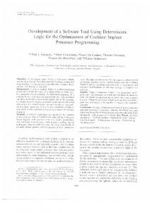
Methods

In this section some methods for reconstructing dihedral angles or amino acids from these probabilistic descriptors are presented and analysed for their potential to find the original angles or amino acid types. In figure 2.2.1 a test program flow is shown for reconstructing dihedral angles. It allows one to compare the constructed angles to the angles of a known structure. The steps are as follows. 1. The protein structure is broken into overlapping fragments of dihedral angles. 2. The fragments are classified, i.e. probability vectors are calculated. 3. The class weights are associated with Gaussians in order to build mixture distributions. 4. From the mixture distributions, dihedral angles are calculated and compared to the original values. 5. A three-dimensional model can be constructed from the dihedral angles and compared to the original structure. 19

Figure 2.2.1: Method for testing the reconstruction capability of a classification. Similarly, the amino acid label reconstruction can be tested.

2.2.1

Dihedral Angles

First some formulae for reconstructing dihedral angles from probability vectors are introduced. A protein structure of length l is represented by a set of l − k + 1
probability vectors v i = vij j∈[1,n] each describing an overlapping fragment xi , where i ∈ [1, l − k + 1]. This raises the problem of combining the overlapping parts. Since there is no rigorous method, several approaches were implemented and tested. Similar to the case of sequence fragments (section 2.2.3 page 26), four principle combinations of the overlaps are proposed, which all have their advantages and disadvantages. Three combinations can be justified in terms of probability estimates. The fourth approach, could be termed an analytical-technical method. The four approaches are named after their primary underlying combination ideas. The three probabilistic approaches are 1. the “geometric mean” (formula (2.2.1)), 2. the “arithmetic mean” (formula(2.2.2)), and 3. the “maximum” approach (formula (2.2.3)), which are introduced one after another in turn. The technical approach is called “inverse Gaussian” and is introduced in paragraph 2.2.1.4 on page 23. 20

2.2.1.1

Geometric Mean T

est Let (φest i , ψi ) denote a pair of estimated dihedral angles and est est est est est T xest = (φest 1 , ψ1 , . . . , φi , ψi , . . . , φl , ψl ) the estimated dihedral angles of the whole protein, then the overlapping parts can be combined by treating them as statistically independent which means multiplying the corresponding probabilities. Normalisation then leads to a geometric mean of the probabilities of an angle pair appearing at different dimensions of the overlapping fragments. Formally given by v     est  Z Z   u Y X n φ φi φ |Iu | t i dφ dψ, (2.2.1) vi′ j pCj X i−i′ +1 = = est ψ ψ ψi i′ ∈I j=1 i

R2

 Xtφ is the bivariate random vector modelling the values of the where X t = Xtψ dihedral angle pair at the tth residue of a fragment. The index set for a residue i of all overlapping fragments xi′ is defined as 

Ii = [max{1, i − k + 1}, min{l − k + 1, i}] and the integrals run over the angles φ and ψ. 2.2.1.2

Arithmetic Mean

The second combination approach is based on the idea that the overlapping parts are actually just different stochastic models accounting for the same variable. That means the corresponding probabilities should be weighted by the respective prior model probabilities and added up. However, as the prior model probabilities are not known, they are assumed to have equal probabilities here. Therefore, the sum is normalised by the number of overlapping models |Ii | leading to an arithmetic mean of the overlapping probabilities. The formula is very similar to the geometric mean approach, but can be simplified to  est     ZZ   n φ 1 XX φi φ = vi′ j pCj X i−i′ +1 = dφ dψ est ψ |Ii | i′ ∈I j=1 ψi ψ i

R2

=

where µj t = class Cj .



µj t φ µj tψ

n XX

1 |Ii | i′ ∈I



i

j=1

vi′ j µj i−i′ +1 ,

(2.2.2)

is the two-dimensional mean vector for the tth residue of

21

2.2.1.3

Maximum

The third approach is similar to the second combination approach in that it also combines the overlapping parts by an arithmetic mean. But instead of calculating the expectation values for each mixture model, the expectation values (i.e. the mean vectors) of the individual classes with highest probabilities are averaged. This is computationally less expensive and formally taken to be  est  1 X φi = µ , (2.2.3) ′ est ψi |Ii | i′ ∈I jmax (i ) i−i′ +1 i

n

where jmax (i′ ) = arg max vi′ j is the index of the class with the highest weight. j=1

From theory it is known, that linear averaging with joint probabilities will not necessarily lead to correct estimates. In section 2.1 it has been shown, that marginal probability densities could lead to better results. With the marginal probability density vectors an arithmetic mean approach can be formulated in est analogy to equation (2.2.2) for φest i and ψi , respectively, by Z n 1 X X marg est φi = φ v′ ′ p (Xi−i′ +1 φ = φ) dφ |Ii | i′ ∈I j=1 i ,i−i +1φ j Cj R

i

n XX

1 = |Ii | i′ ∈I =

i

j=1

n XX

1 |Ii | i′ ∈I

j=1 n XX

1 ∧ ψˆi = |Ii | i′ ∈I

vimarg ′ ,i−i′ +1 φj

Z

φ pCj (Xi−i′ +1 φ = φ) dφ

R

vimarg µj i−i′ +1φ ′ ,i−i′ +1 φ

(2.2.4φ )

vimarg µj i−i′ +1ψ . ′ ,i−i′ +1 ψ

(2.2.4ψ )

j

i

i

j=1

j

In similar ways the geometric mean and maximum approaches, i.e. formulae (2.2.1) and (2.2.3), can be reformulated using marginal probability density vectors est T est by replacing (φest or ψiest and vi′ j with vimarg or vimarg ′ ,i−i′ +1 ′ ,i−i′ +1 i , ψi ) with φi φj ψj   T and pCj X i−i′ +1 = (φ, ψ) with pCj (Φi−i′ +1 = φ) or pCj (Ψi−i′ +1 = ψ), respectively. This leads to the geometric mean approach for marginal probability density vectors v uY X Z n u est It | | i φi = φ vimarg (2.2.5φ ) pCj (Φi−i′ +1 = φ) dφ ′ ,i−i′ +1 φ R

∧ ψiest =

Z R

i′ ∈Ii j=1

j

v uY X n u It | | i vimarg pCj (Ψi−i′ +1 = ψ) dψ, ψ ′ ,i−i′ +1 ψ i′ ∈Ii j=1

j

22

(2.2.5ψ )

and the maximum approach based on marginal probability density values 1 X (2.2.6φ ) µj φest ′ i = |Ii | i′ ∈I max i−i +1φ i X 1 ∧ ψiest = µj . (2.2.6ψ ) ′ |Ii | i′ ∈I max i−i +1ψ i

These approaches are also tested with linearised weights as suggested in subsection 2.1.1.3, page 15. 2.2.1.4

Inverse Gaussian

Here the fourth rather technical approach to reconstructing dihedral angles from probability vectors is introduced and later analysed for its performance. The inverse Gaussian approach is not justified in probabilistic terms, but rather analytically derives the original angles from their probability functions. First the inverse Gaussian approach is developed using joint probabilities. The basic idea for the inverse Gaussian approach is to construct an inverse formula by solving the following equation system for the unknown angles xi . i h T −1 1 exp − 2 (xi − µ1 ) C 1 (xi − µ1 ) nonorm p vi 1 = w 1 (2π)2k | det C 1 | .. . h
T i
−1 1 exp − 2 xi − µj C j xi − µj p ∧ nonorm vi j = wj (2π)2k | det C j | .. . h i T exp − 21 (xi − µn ) C −1 (x − µ ) i n n p ∧ nonorm vin = wn (2π)2k | det C n |

A univariate inverse Gaussian would lead to two possible angle values, left and right from the class mean. To decide which angle is the correct one a second univariate inverse Gaussian (a second class) is needed giving another two possible angle values. Two values of these four possible values are equal or at least very similar and can be interpreted as the wanted angle. As illustrated in subsection 2.1.1.1, page 12, for two dimensions the equation system results in either 0, 1, 2, 3 or 4 solutions (an infinite number of solutions does not occur, as µj 6= µj ′ holds for all j ′ 6= j). But as the equation system is over-defined (many more classes than angles to be estimated, i.e. n ≫ 2k), a single solution could be found this way. In general, multivariate Gaussians are used to model multivariate classes of fragments of length k consisting of 2k dihedral angles. As shown in 23

paragraph 2.1.1.1 for two dimensions, one 2k-variate inverse Gaussian would lead to a 2k-dimensional ellipsoid for a given function value (also called a contour), i.e. the solutions for a single equation lie on a hyperellipsoid of dimension 2k. The formulae are very large and are not given here explicitly. The common points of two such ellipsoids (if they form an equation system) would describe either • • • • • • •

a 2k − 1-dimensional ellipsoid, a single point, two 2k − 1-dimensional ellipsoids, two single points, one 2k − 1-dimensional ellipsoid and one point, the original ellipsoid or no point.

However, the last two cases can be excluded, because the equation system is assumed to be solvable (at least approximately) since it was constructed from a single vector xi and the ellipsoids come from different classes. In order to determine the wanted angle values, a minimum of 2k + 1 2k-variate Gaussians is needed. Although, the number of classes n is much higher then their dimension 2k, it is not guaranteed to find a unique solution. The solution becomes much simpler when the unnormalised marginal probability vectors are used for the following equation system (for ψ angles this looks analogous).

nonorm marg vi,tφ 1

= w1

"

exp −

.. .

∧

⇐⇒

∧

nonorm marg vi,tφ n

µ1 t φ

µn t φ

= wn

v u u ± t−2c1t

v u u ± t−2cnt

φ ,tφ

φ ,tφ

exp −

log

" "

φi+t−1 −µ1 t

φ

2c1tφ ,tφ

p 2πc1 tφ ,tφ

"

log





φi+t−1 −µn t 2cntφ ,tφ

p 2πcntφ ,tφ

2 #

φ

2 #

nonorm v marg q i,tφ 1

w1

nonorm v marg q i,tφ n

wn

24

2πc1tφ ,tφ

2πcntφ ,tφ

# #

= φi+t−1 .. . = φi+t−1

(2.2.7)

A single equation results in two possible values and the common value of the system (if any) should be the desired angle. Theoretically this may to lead to exactly reconstructed angles. For results on these formulae for dihedral angle reconstruction see section 2.3.2.

2.2.2

Backbone Reconstruction

Using the bond lengths and the bond angles from the literature [EH91, HBA+ 07] or from a known protein structure a full atom representation of the protein backbone can be build solely by knowing the dihedral angle sequence. This should work, because the amide plane is known to be a relatively rigid unit, see figure 1.3.1, page 6. Here, the same method as in [Mah09] is used to convert a sequence of dihedral angles to Cartesian coordinates of atoms and bonds. It basically takes any full atom representation of the desired length with arbitrary dihedral angles. The difference between these and the new dihedral angles is calculated and then imposed by several rotational and translational moves. When calculating Cartesian coordinates from a given sequence of φ- and ψ-angles the unknown bond lengths and bond angles as well as the torsional ω-angle have to be guessed, see figures 1.1.1 on page 2 and 1.3.1 on page 6. However, compared to the variation in φ and ψ and the length of proteins, these values actually vary only very little and are assumed the be fixed. It is rather interesting to see how much error is introduced due to this approximation [EH91, HT04, BSDK09]. To investigate this for our implementation, the dihedral angles of known protein structures (the PDBSelect50 subset [PDBb]) are extracted and then the unknowns can be taken either from another, sufficiently long, protein structure (e.g. 2FHF), the literature (i.e. a polyalanine model constructed by USCF Chimera [PGH+ 04]) or from the known structures themselves, respectively. The comparison of the generated structures to the target structures reveals the introduced reconstruction error. The procedure is as follows for each structure in the test set: 1. extract the φ, ψ sequence from the known structure 2. set all φ and ψ angles to zero in a copy of the known structure, so that the structure becomes completely extended 3. do the same for 2FHF and the polyalanine and shorten the polymers to the size of the known structure 4. set the φ and ψ angles to the previously extracted values in the copied structure, 2FHF and the polyalanine 5. compare all three structures to the original unmodified target structure 25

2.2.3

Amino Acids

In this section reconstruction approaches for the discrete sequence terms are introduced. In analogy to the structural fragments the protein sequence is broken into overlapping fragments for which probability vectors are calculated (figure 2.2.1 page 20). From these, the original amino acid labels are reconstructed in order to get a feeling for the crudeness of the simplification due to the Bayesian classification.
According to [SMT08b, CS96] the elements of the probability vector v i = vi j j∈[1,n] for a sequence fragment si of length k are given by wj pCj (S = si ) vij = psi (F ∼ Cj ) = p(F ∼ Cj |S = si ) = P n wj ′ pCj′ (S = si )

(2.2.8)

j ′ =1

and can be interpreted as the n-dimensional vector of probabilities of all n classes Cj given the sequence si . The prior class weights wj are directly taken from the k Q classification and pCj (S = si ) = pCj (St = sit ) is the product of the 20-way t=1

Bernoulli probabilities. As amino acid labels are nominal features, averages or expectation values to construct the amino acid labels from the probability vectors (as done for dihedral angles) are not defined. One way to find a representative is to search for the class with the highest probability at each residue. This leads to the construction formula for the estimated amino acid label si est at the tth t residue of the sequence fragment si , given by si est t

20

= arg max a=1

n X j=1

vij pCj (St = a),

(2.2.9)

where arg max f(a) = amax : f(amax ) ≥ f(a) ∀a and the weighted sum forms the a mixture distribution for amino acids. However, a protein sequence of length l is represented by a set of l − k + 1 probability vectors each describing an overlapping fragment si where i ∈ [1, l − k + 1]. This raises the problem of combining the overlapping parts. There exists no sensible way to combine amino acid types, but the corresponding probabilities can be combined. As for the reconstruction of dihedral angles the same three probabilistic ways and one analytical-technical approach are investigated here for the same reasons as stated in section 2.2.1. They are given as extensions on est est T formula (2.2.9) using the notation sest = (sest 1 , . . . , si , . . . , sl ) for the estimated protein sequence. The linear weighted average over all classes stays for the geometric mean and the arithmetic mean approaches. However, the averaging of the overlapping parts is dropped as the absolute values are enough for finding the amino acid label with maximal probability. 26

2.2.3.1

Geometric Mean

Considering the overlapping parts as independent random variables leads to the geometric mean or product approach, which is taken be sest i

20

= arg max a=1

n YX

i′ ∈Ii j=1

vi′ j pCj (Si−i′ +1 = a),

(2.2.10)

where Ii is the index set for a residue si of all overlapping fragments si′ , formally given by Ii = [max{1, i − k + 1}, min{l − k + 1, i}]. 2.2.3.2

Arithmetic Mean

The arithmetic mean or sum approach is based on the idea that the overlapping parts are different models for the same random variable and is formulated by sest i

2.2.3.3

20

= arg max a=1

n XX

i′ ∈I

i

j=1

vi′ j pCj (Si−i′ +1 = a).

(2.2.11)

Maximum

The maximum approach for amino acids looks a little bit different to the maximum approach for dihedral angles, but it follows the same idea. Estimate the  20 unknown label by taking the representative arg max with the highest proba=1     n and all classes max . Formally ability over all overlapping fragments max ′ j=1

i ∈Ii

written

20

n

max vi′ j pCj (Si−i′ +1 = a). sest i = arg max max ′ a=1 i ∈Ii

2.2.3.4

(2.2.12)

j=1

Inverse Calculation

The fourth rather technical approach to construct the amino acid sequence from probabilities uses marginal probability vectors, similar as in subsection 2.2.1.4 for dihedral angles. The idea is to find the amino acid that led to the probability values by inverse calculation. The unnormalised marginal probability vector for an amino acid sequence fragment si is defined by
nonorm v i = nonorm vij t j∈[1,n]∧t∈[1,k]   = wj pCj (St = si t ) , (2.2.13) j∈[1,n]∧t∈[1,k]

27

where i is the index of the first residue in the fragment, k is the length of the fragment and n is the number of classes. n

′

i,i = arg max Let jmax

nonorm v

i′ j i−i′ +1

wj

j=1

be the class having maximal probability for

fragment i′ at the mutual residue i − i′ + 1 with fragment i. Then i′max = nonorm v

arg max ′ i ∈Ii

i′ i,i′ jmax i−i′ +1

wj

is the overlapping fragment with the highest probability

for that class. With this the amino acid label for the residue i can be estimated using marginal probability vectors by 20

sest i = arg max pC i,i′ a=1

max jmax


Si−i′max +1 = a .

(2.2.14)

For results on these formulae for sequence reconstruction see section 2.3.3. 2.2.3.5

Substitution Matrix

The comparison of a substitution matrix calculated from a set of generated sequences to an established matrix like blosum [HH92] summerises some interesting properties of our method. It shows which substitutions are under- or overrepresented and the correlation coefficient quantifies how close the sampled sequences are to being biologically relevant. In order to calculate a substitution matrix from a pool of generated sequences, the relative frequencies of aligned amino acids pab and the relative frequencies of seeing this cooccurrence by chance pa pb have to be extracted from the sequence pool. According to [HH92] the matrix entries are then given by   1 pab sab = log , λ pa pb where λ is a scaling factor.

2.3

Results

A few classifications have been tested. Depending on the classification the results are different, but the trends stay the same. Therefore, the evaluation is restricted to a classification that did reasonably well in other projects, e.g. comparing proteins. It consists of 162 classes for fragments of length five. In this classification five Gaussian distributions cross the periodic boundary of the ψ angles (class mean ± deviation) at − π2 . No class crosses the φ boundary at 0 and no class spans more than one period. 28

80

35

70

30

60

25

50

20

40

15

30

10

20

5

10

0

Cα -RMSD [˚ A]

φ- and ψ-RMSD [rad·10−5 ]

40

0 original φ

2FHF

polyALA Cα

ψ

Figure 2.3.1: Reconstruction of all structures of the PDBSelect50 subset [PDBb] using their φ- and ψ-angles and either their original geometries, the geometry of 2FHF or a poly-Alanine model, respectively. The boxes indicate the 1st (25%), 2nd (median) and 3rd (75%) quartiles and the whiskers the minimum and maximum.

2.3.1

Influence of Bond Lengths and Angles

Figure 2.3.1 quantifies the influence of bond lengths and angles on the reconstructed coordinates of the PDBSelect50 subset using the original dihedral angles φ and ψ. As expected all modified structures with native geometry have no difference to the original structures, respectively, besides precision errors. The modified structures with the geometry of 2FHF have significantly large root mean squared deviations on the α-carbon positions (Cα -RMSD). The situation with the idealised geometry (polyalanine) does not look much different as seen in figure 2.3.1. For a discussion on these issues see section 2.4.1 on page 34.

2.3.2

Dihedral Angle Reconstruction

In order to demonstrate the potential of the formulae introduced in section 2.2.1 the reconstructed dihedral angles are compared to the native values of a few example structures. Four approaches are tested altogether. Two approaches are probabilistic using joint probability vectors, namely the arithmetic mean (formula (2.2.2)) and the maximum approach (formula (2.2.3)). One probabilistic 29

π

π 2

π 2

0

0

ψ

ψ

π

− π2

−π −π

− π2

− π2

0

φ

π 2

−π −π

π

π

π

π 2

π 2

0

0

π 2

π

− π2

− π2

−π −π

0

φ

(b) maximum on joint probabilities, φ-RMSD: 0.421 (24.1◦ ), ψ-RMSD: 0.467 (26.8◦ ), Cα -RMSD: 27.406˚ A

ψ

ψ

(a) arithmetic mean on joint probabilities, φ-RMSD: 0.422 (24.2◦ ), ψ-RMSD: 0.479 (27.5◦ ), Cα -RMSD: 17.773˚ A

− π2

− π2

0

φ

π 2

−π −π

π

(c) arithmetic mean on marginal probabilities with linearised weights, φ-RMSD: 0.239 (13.7◦ ), ψ-RMSD: 0.283 (16.2◦ ), Cα -RMSD: 22.188˚ A

− π2

0

φ

π 2

π

(d) inverse Gaussian on marginal probabilities with linearised weights, φ-RMSD: 0.276 (15.8◦ ), ψ-RMSD: 0.539 (30.9◦ ), Cα -RMSD: 17.880˚ A

Figure 2.3.2: Four φψ plots of the dihedral angles of the protein 1AKI. Shown in red are the actual target values and in blue the values estimated by using an arithmetic mean (a), using a maximum of the overlapping parts (b), using marginal probabilities with an arithmetic mean of the overlapping parts and with linearised weights (c) and using marginal probabilities with the technical inverse Gaussian approach (d), respectively.

30

200

2.5

160

2

140 120

1.5

100 80

1

60

Cα -RMSD [˚ A]

φ- and ψ-RMSD [rad]

180

40

0.5

20 0

0 (2.2.2)

(2.2.3)

φ

ψ

(2.2.4)

(2.2.7)

Cα

Figure 2.3.3: Performance of four reconstruction formulae tested on the PDBSelect50 subset [PDBb]. (2.2.2): arithmetic mean on joint probabilities, (2.2.3): maximum on joint probabilities, (2.2.4): arithmetic mean on marginal probabilities with linearised weights, (2.2.7): inverse Gaussian on marginal probabilities with linearised weights. The boxes indicate the 1st (25%), 2nd (median) and 3rd (75%) quartiles and the whiskers the minimum and maximum. approach, the arithmetic mean, is also tested with marginal probabilities and linearised weights (formula (2.2.4) combined with formula (2.1.7)). And finally the fourth rather technical approach uses inverse Gaussians (formula (2.2.7)). Results for the other approaches are not shown, because either they take very long to obtain (integration in the geometric mean approaches) or they are not very different to the results presented here. From the probability vectors for structure 1AKI the dihedral angles are reconstructed and compared to the original values. Figure 2.3.2 shows their distributions in scatter plots for each tested formula. In almost all four plots the generated angles fall into the three prominent regions, right-handed helical, strand and lefthanded helical. The deviations to the original values seem to be equally high for the two probabilistic approaches using joint probability vectors. Although they differ in their Cα -RMSD, the dihedral angle difference between the arithmetic mean and maximum approach is only very little as seen in plots 2.3.2a and 2.3.2b. The four approaches are also tested on the whole PDBSelect50 subset [PDBb]. The results are shown in figure 2.3.3. The arithmetic mean approach with marginal probabilities and linearised class weights yields the lowest dihedral angle 31

protein sequence 1TU7A 1FC2C 1ENH 4ICB 1BDD 1AKI 2GB1 1HDDC

performance of formula [%] (2.2.10) (2.2.11) (2.2.12) (2.2.14) 38 38 33 76 42 42 40 79 33 33 37 74 54 55 49 82 40 40 35 82 36 35 27 72 41 43 36 91 33 32 35 72

Table 2.3.1: Reconstruction of a few example sequences. (2.2.10): geometric mean on joint probabilities, (2.2.11): arithmetic mean on joint probabilities, (2.2.12): maximum on joint probabilities, (2.2.14): inverse calculation on marginal probabilities. RMSDs on average. Again the arithmetic mean and the maximum approach with joint probabilities perform equally well on this dataset. On average these two approaches also show no significant difference in Cα -RMSD. In section 2.4.2 the dihedral angle reconstruction results are discussed.

2.3.3

Sequence Reconstruction

In order to demonstrate the potential of the statistical description of the protein sequence, the three probabilistic approaches from section 2.2.3, geometric mean (formula (2.2.10)), arithmetic mean (formula (2.2.11)) and maximum (formula (2.2.12)) with joint probabilities as well as the technical inverse calculation (formula (2.2.14)) with marginal probabilities are tested on a few example sequences and on the large PDBSelect50 subset [PDBb]. The calculated sequences are compared to the native sequences, see table 2.3.1 and figure 2.3.4. The similarity for the technical reconstruction approach (formula (2.2.14)) is highest for all sequences. The other, probabilistic approaches perform significantly worse, but give similar results compared to each other. The average performance of reconstruction of the arithmetic mean approach (formula (2.2.11)) is 41% sequence identity (figure 2.3.4). A matrix calculated from the observed substitutions is shown in table 2.3.2 (lower triangle). The difference to the blosum 40 matrix is shown in the upper part of the same table. The strong negative entries in this difference matrix originate from substitutions that were not observed for the arithmetic mean approach. The correlation coefficient is 0.15. The average reconstruction performance for the inverse calculation approach (formula (2.2.14)) is 93% sequence identity and the correlation coefficient of its substitution matrix and the blosum 90 matrix is 0.5. 32

A R -4 2 -10 A 1 R 0 -1 N 0 -3 D -1 -1 C -1 -8 Q 0 -3 E 0 0 G -2 -1 H 0 -3 I -3 -8 L 0 0 K 0 0 M -1 -8 F -2 -8 P -1 -1 S 0 -1 T 0 -2 W -1 -8 Y -1 -8 V -1 0 A R

N D C Q 1 0 1 0 -3 0 -5 -5 -8 -1 -6 -3 -8 2 0 0 -23 -4 1 1 -9 -8 0 -7 -2 -1 -8 -1 0 0 -2 0 1 0 -1 -1 -2 0 -7 -3 -8 -3 -8 -8 -1 -2 0 0 -1 -1 -8 0 -8 -2 -7 -8 -8 -1 -8 -8 -2 -1 -2 -1 -1 0 -1 -1 -2 0 -1 -2 -8 -1 -7 -8 -8 -1 -7 -8 -1 -2 0 0 N D C Q

E G H I L K M F P S T W Y V 1 -3 2 -2 2 1 0 1 1 -1 0 2 1 -1 1 2 -3 -5 2 -3 -7 -6 2 0 0 -6 -7 2 1 1 -3 -6 2 -1 -6 -5 0 -2 -2 -4 -6 2 -2 2 0 1 1 -1 1 3 1 0 1 4 2 1 0 2 -3 -4 2 -5 -4 -6 3 0 0 -1 -3 2 -2 1 -3 -5 2 -1 -7 -4 1 -2 -1 -7 -7 3 -6 1 0 2 1 -1 1 2 -1 0 1 1 1 2 -7 2 1 0 1 0 1 -2 0 0 0 1 1 1 -20 -5 2 0 -9 -6 0 0 0 4 -10 4 -2 1 -9 -2 -5 -9 -9 0 -1 -7 -5 -8 -4 0 0 -7 -6 2 -3 -2 2 3 1 1 0 -2 -2 -3 -8 -3 -5 -1 0 1 -1 -1 -1 -1 1 -1 -4 0 0 0 -14 -8 0 0 -2 -5 -9 -1 0 -1 -1 -8 0 1 -17 2 -1 -7 -3 -12 0 -1 -2 -8 -8 0 -2 -7 -10 0 -1 3 1 1 -1 -2 -8 -8 0 -3 -8 -8 -4 -2 3 0 0 -1 -3 -2 -2 -2 0 -2 -2 1 -5 -2 -3 -5 0 0 -1 -3 0 -1 -2 -3 -1 1 -19 -5 3 0 -2 -2 -8 0 -1 -3 -8 -1 0 1 -17 1 -1 -2 -1 -8 0 -3 -7 -2 -1 -2 -8 0 -4 -1 -2 -8 -8 0 -2 -8 -8 -2 -2 -3 -2 -8 -1 -3 0 0 0 -1 0 0 -2 -1 0 0 0 1 E G H I L K M F P S T W Y V

A R N D C Q E G H I L K M F P S T W Y V

Table 2.3.2: Substitution matrix for the arithmetic mean approach, formula (2.2.11), (lower triangle) and difference matrix (upper triangle) obtained by subtracting the blosum 40 matrix [HH92] position by position.

33

sequence identity [%]

100 80 60 40 20 0 (2.2.10)

(2.2.11)

(2.2.12)

(2.2.14)

Figure 2.3.4: Sequence reconstruction of the PDBSelect50 subset [PDBb] using four different reconstruction formulae, respectively. (2.2.10): geometric mean on joint probabilities, (2.2.11): arithmetic mean on joint probabilities, (2.2.12): maximum on joint probabilities, (2.2.14): inverse calculation on marginal probabilities. The boxes indicate the 1st (25%), 2nd (median) and 3rd (75%) quartiles and the whiskers the minimum and maximum. In section 2.4.3 the sequence reconstruction results are discussed.

2.4 2.4.1

Discussion Influence of Bond Lengths and Angles

The influence of the bond lengths and angles on the quality of the results is quite strong. Using literature values for them leads to rather large Cα -RMSDs. There seems to be a significantly high variation [BSDK09] and one should consider using amino acid specific bond angles and lengths. This might slightly improve the results. Despite the errors introduced by bond angles and lengths, the dihedral backbone angle ω is known to vary by a few degrees and completely points to opposite directions for Proline residues (cis-conformation of the peptide bond). In order to minimise error originating here the ω-angles should be set at least dependent on the amino acid type. 34

2.4.2

Dihedral Angle Reconstruction

Here, a few properties of the dihedral angle reconstruction approaches are discussed. It is important to note that, besides the approximations caused by using standard bond geometries, a few wrong dihedral angles may lead to high Cα RMSDs. In figure 2.3.2 the dihedral angles RMSDs and the Cα -RMSDs seem not to correlate with each other. Another principle observation concerning the Cα -RMSD is that it may get incredibly high, up to 180˚ A in figure 2.3.3. With high evidence this is due to bad structures. The WURST library used can only deal with single-chained proteins without gaps [TPH04]. If these structures were filtered out, the generated structure model will tend to have lower Cα -RMSDs. The difference between the performance of the arithmetic mean and the maximum approaches on joint probabilities is only very little. This means that each fragment has a high preference for one single class, as the averaging in the arithmetic mean approach (formula (2.2.2)) does not change the results significantly. This finding is consistent with other work [Hof07], where the probability vectors could be compressed using only very few classes in order to build structural alphabets. It also suggests that the classes cover the data quiet well. This does not mean there are no weird angles in the data, but they rather lie in between classes and are covered by a mixture of a few moderately populated classes. Surprisingly, the inverse Gaussian approach does not lead to an exact reconstruction, although this is expected by construction of the formulae. Checking very carefully the numbers, it turns out, that if the class means are very close to the original value, then the angle can be reconstructed quite reliable. However, most class means are significantly far away from the original angle leading to strong precision errors, i.e. the values for one angle deviate quite a lot. Averaging over these numbers necessarily results in badly reconstructed angles. Maybe replacing the average by a weighted average, e.g. using the class weights, would improve the reconstruction. The other approach, the arithmetic mean on marginal probabilities with linearised weights, is also exact by construction but seems to have similar problems. However, there are additional issues to be considered. The original angles often lie close to the boundaries. These angles are smaller (or larger) than any class mean. Taking a weighted average between any two class means would not lead to the desired angle. Even using periodic images would not help here, as the class weights were calculated within a single period only. Calculating class weights of two periods would help here. However, an even better solution would be to change the classification model to use periodic probability distributions, like the von-Mises models. This was not done in this work in order to use existing classifications built for other projects [SMT08b, MST09]. Extending this would require a lot of careful programming, but is strongly recommended for future projects. 35

The exact approaches are interesting for reconstruction, but unfortunately are unsuitable for structure prediction where the probability vectors come from sequence. There the assumption that the class weights may be interpreted to reflect some sort of distance of the wanted angle to the class means does not hold. The weights should rather be regarded as class probabilities. For example, if two classes have positive probability, then the angle does not lie only in between the class means but is likely to be found anywhere around the class means with respect to their density distributions. Taking the arithmetic mean (formulae (2.2.2) and (2.2.4)) of the overlapping parts is theoretically and practically the most reasonable approach. The overlapping fragments are treated effectively as a random variable of different stochastic models for the dihedral angles. Each expression has equal probability. But this could be changed easily, see also final discussion chapter 6, page 87. Considering the use of marginal probability vectors results in lower RMSD values here, however the loss of correlated features leads to limited applicability for sampling approaches (section 4.1.2.1, page 52).

2.4.3

Sequence Reconstruction

Using the pairwise sequence identity to the native sequence as a quality measure for the reconstructed sequences leads to rather conservative numbers. The numbers are lower than expected from a biological point of view. This measure underestimates the biochemical similarity of the sequences. Instead of the plain identity, a similarity score based on substitution matrices like pam or blosum would better reflect the biological relevance of the generated sequences. However, choosing the correct matrix is dependent on the evolutionary distance between the sequences. But, the true (substitutional/mutational) distance between sequences folding to similar structures was not investigated here. Using the average identity of the generated sequences as an approximation of the evolutionary distance would not help, as it would not lead to a measure telling us how realistic the generated sequences are. The best way to check the relevance of the generated sequences would be to synthesise them and determine their structure experimentally, but this is not feasible. However, on the computer sets of native sequences from the same structure cluster (fold) could be analysed in order to see if the generated sequences can be found there. For each fold a sequence profile could be built, which could serve as an estimate of the true variation. Subsequently, this profile could be compared to our substitution matrices. The low correlation between our substitution matrices and the established matrices suggests that there is only very little similarity in the substitution patterns 36

and the potential of the classification is limited for some affected amino acids. Comparing the substitution matrices from our reconstruction formulae to the blosum 40 or blosum 90 matrices is actually not perfect. The blosum x matrices are generated from a pool of sequence alignments with less than x% sequence identity. As the sequence identity of our generated sequences spans a range from 0 to 100%, the observed substitutions actually should be compared to either the blosum 100 matrix or, all sequences with more than x% identity should be clustered first and then compared to blosum x. Additionally, there is also the problem of scaling. To avoid that, a rank correlation coefficient could be calculated. But overall the values would roughly stay the same, since these numbers are dependent on the scoring, which is intentionally kept very simple. Our scoring is solely based on structural features, whereas blosum also considers effects of evolution implicitly. Nevertheless, it would be nice to have a measure for how close the pool of generated sequences is to the natural pool of sequences folding to similar structures. This would become also relevant in the light of more sophisticated scoring functions. A median of 93% sequence identity for the set of sequences generated by the technical approach (formula (2.2.14)) can be considered the limit of what is possible to reconstruct using the classification. It is clear, that a classification is always a simplification. Here that means, that some amino acid sequences are so similar, that they form a motif in the classification and, therefore, can no longer be distinguished or reconstructed. This has also consequences for the construction and comparison of substitution matrices. Some substitutions are put together already in the classification and therefore can not be observed in the substitution matrix. Of course, this further lowers the correlation coefficients to the established matrices. The technical approach yields the highest reconstruction rate. However, this has no meaning if the probabilities come from a protein structure. This will become relevant for sequence prediction (chapter 5). Instead, the probabilistic approaches have the advantage, that they can also be used sensibly with probability vectors created from structure. From these the arithmetic mean approach (formula (2.2.11)) seems to be the best choice for the sequence prediction task. Its calculation is simple and it can be justified most rigorously in statistical terms. The overlapping parts are effectively treated as statistical variables that can take different mixture models as values.

37

38

Chapter 3 Self-consistent mean field optimisation In this chapter an innovative optimisation method for finding self-consistent states introduced for systems that are described by a probabilistic mean-field model [ST]. It is especially suited, but not limited to our Bayesian classification based on overlapping protein fragments. Predicting unknown features such as structure or sequence basically means to optimise the population of their states. The method described here is applied in the following chapters and allows to efficiently explore the conformational or compositional space of proteins. Self-consistent mean field (SCMF) methods [KD96] have traditionally been used to optimise wave functions [Sto05] and have been applied to a variety of problems [HKL+ 98, MBCS01, MM03, Edw65, Dew93, RFRO96, KD98, SSG+ 00, DK97, CdMaT00, XJR03]. In all these applications, the system is subdivided into small subsystems which can interact through a mean field. One assumes the system to be in all states at the same time and iteratively updates the contribution of each state to the mean energy field through the Boltzmann relation. This process consists of alternating steps of calculating the mean energy of a subsystem and its interacting subsystems, updating the probabilities of each state of the subsystem, recalculating the energy and so on. These steps are iterated over all subsystems until a self-consistent state of the whole system is found. This state is reached when the probabilities of the states of the subsystems converge, i.e. they no longer change. In order to describe the mean field previous studies invented energy functions, which are more or less directed by human preconceptions. Especially the selection and relative weighting of terms is an optimisation task in itself. In contrast, this study introduces a purely statistical version of SCMF using rather simple scoring terms. It uses the idea of overlapping subsystems and works with conditional 39

probabilities directly without using the Boltzmann relation. First, the standard procedure is described and some basic notation is introduced. Then, a description of the purely statistical version follows. Finally, a new cooling scheme is introduced. It adaptively lowers the entropy of the system via a temperature-like convergence parameter. Applied to our statistical SCMF version this leads to a method that smoothly narrows down the solution space.

3.1

Standard SCMF

Self-consistent mean field methods aim to find the state of lowest energy. The standard method assumes a conventionally defined energy function and is therefore extended in this work (section 3.2). It is described here for comparison. The system X is divided into small disjoint subsystems Xi . Each subsystem is considered to be in all possible states Si = {xi } at once with a certain probability p(Xi = xi ). This probability is adapted via an iterative procedure until the system converges to a self-consistent state, i.e. the probabilities no longer change. The energy function that one seeks to minimise is taken to be XX Eeff (X, p) = p(Xi = xi ) EXi (xi ). i

xi ∈Si

Each subsystem Xi in state xi feels the influence of its surrounding subsystems Xi′ in a mean field, given by the mean interaction energy X X p(Xi′ = xi′ ) EXi Xi′ (xi , xi′ ), EXi (xi ) = i′ 6=i xi′ ∈Si′

where EXi Xi′ (xi , xi′ ) is the pairwise interaction of Xi being in state xi and Xi′ being in state xi′ . Ideally, this interaction should be calculated among all subsystems. However, in practice, either the energy function is not defined for long-range interactions or the calculation will lead to a combinatorial explosion. Therefore, the mean interaction energy is typically calculated on some subset {Xi′ | i′ ∈ Oi } of closely interacting subsystems, leading to X X EXi (xi ) = p(Xi′ = xi′ ) EXi Xi′ (xi , xi′ ). (3.1.1) i′ ∈Oi xi′ ∈Si′ i′ 6=i

In each iteration step the mean interaction energy of each subsystem in each particular state and the mean field of its surrounding subsystems is calculated and then turned into probabilities using the Boltzmann relation, given by exp (−β EXi (xi )) p(Xi = xi ) = P , exp (−β EXi (x′i )) x′i ∈Si

40

(3.1.2)

Rki′ ,i Rui′ ,i

O ki′ ,i O ui′ ,i O ki,i′ O ui,i′

Rki,i′ Rui,i′ 



Figure 3.2.1: Notation for two overlapping systems Xi′ = Rki′ ,i , Rui′ ,i , Oki′ ,i , Oui′ ,i and Xi = 

 O ki,i′ , O ui,i′ , Rki,i′ , Rui,i′ .

where β is the inverse, Boltzmann-weighted temperature. In order to distinguish from a single iteration step, a loop over all subsystems and all states is called a simulation step. Ideally, the procedure finds a single self-consistent state of the system after several simulation steps. In general, the system will find itself in a number of states. In order to decrease the number of possible states, one can gradually lower the temperature of the system like in simulated annealing [KGV83], see section 3.3.

3.2

Purely statistical SCMF

Instead of using some physical or knowledge-based energy function a purely statistical score function based on conditional probabilities is applied. This allows one to quickly sample the state space without the Boltzmann formalism. In order to achieve this, the standard SCMF protocol is modified. The system is divided into overlapping subsystems, i.e. parts of a subsystem are also modelled in other subsystems. As a consequence, this overlap enables the use of conditional probabilities. That means, the effect that a subsystem has on another can be modelled statistically rather then by some (sometimes arbitrarily simplified) interaction energy. Let us assume statistics on subsystems of systems where the states are known have been collected by treating the subsystems independently and let there be enough statistical data to sufficiently cover the population. Then, the probability of a subsystem being in a specific state can be estimated by fitting its relative frequency to some function p. Let Xi and Xi′ be the two vectors describing the two subsystems that include sites Xi and Xi′ as the first dimensions, respectively (assuming sorted dimensions), and let Xi′ overlap with Xi . Denote the overlapping parts with O i,i′ and O i′ ,i and the rest of the subsystems with Ri,i′ and Ri′ ,i , respectively. Furthermore, assume some observation has been made on an unknown system, then the subsystems can be further split into known and unknown variables, denoted by Xk
and Xu , respectively (see figure 3.2.1). The current probability pcur Xui = xui Xk of the unknown variables of a single site Xui being in state xui is effected by all subsystems overlapping with the subsystem Xi , 41

given by the index set Oi . This effect can be captured by

pcur Xui

=

xui

X

k




Y Y  ′  T2 pold(Xui′ = xui′ pi,i xi ,xi′

i′ ∈Oi xi′ ∈Si′ i′ 6=i

=X Y Y  x∈Si i′ ∈Oi xi′ ∈Si′ i′ 6=i

′ pi,i x,xi′

Xk )

 T2 pold(Xui′ = xui′

Xk )

(3.2.1)

′

where the interaction term pi,i xi ,xi′ reflects the net probability contribution of the u u unknown pair xi , xi′ on the average or marginal probability of the known pair xki , xki′ . In analogy to [Sip90] this is taken to be
p Xki = xki , Xki′ = xki′ Xui = xui , Xui′ = xui′ i,i′
pxi ,xi′ = , p Xki = xki , Xki′ = xki′ with the marginal probability


p Xki = xki , Xki′ = xki′ = p Xki = xki Xki′ = xki′ p Xki′ = xki′
1 X p Oik′′ ,i 1 = xki Oik′′ ,i′ 1 = xki′ = |Ii | i′′ ∈I i   X 1 k k · p Oi′′ ,i′ 1 = xi′ , |Ii′ | i′′ ∈I i′

and the conditional probability
p Xki = xki , Xki′ = xki′ Xui = xui , Xui′ = xui′
= p Xki = xki Xki′ = xki′ , Xui = xui , Xui′ = xui′
· p Xki′ = xki′ Xui = xui , Xui′ = xui′
= p Xki = xki Xui = xui , Xi′ = xi′
· p Xki′ = xki′ Xui = xui , Xui′ = xui′
1 X = p Oik′′ ,i 1 = xki Oiu′′ ,i 1 = xui , Oi′′ ,i′ 1 = xi′ |Ii | i′′ ∈I i
1 X · p Oik′′ ,i′ 1 = xki′ Oiu′′ ,i 1 = xui , Oiu′′ ,i′ 1 = xui′ . |Ii′ | i′′ ∈I i′

Ii is the index set of the subsystems modelling the site Xi . A derivation from formulae (3.1.1) and (3.1.2) is trivial if setting ′

EXi Xi′ (xi , xi′ ) = −β −1 ln pi,i xi ,xi′ .

(3.2.2)

In order to control the entropy of the system a convergence parameter T is introduced, which allows one to simulate cooling effects, just like temperature in 42

simulated annealing [KGV83]. At high T , the probabilities are spread out. As T goes down, the probabilities become more concentrated in the likelier states and probabilities of less populated states will tend to zero, so that the system will end up in the most populated states (see chapter 3.3). The response of a system is not instantaneous. Changes in one part of the system take some iterations to reach other parts of the system. This can lead to oscillations in the probabilities. To avoid this problem, the state probabilities are updated slowly using a memory factor λ ∈ [0, 1]. This leads to


pnew Xui = xui Xk = λ pold Xui = xui Xk + (1 − λ) pcur Xui = xui Xk . (3.2.3)

Iterative application of formulae (3.2.1) and (3.2.3) will populate the sites at states that are consistent with the states at the modelling subsystems, just like in standard SCMF. Interestingly, in contrast to [DK97, Sip90] the method does not need the Boltzmann relation and does not assume the underlying data to be sampled from some well-defined statistical ensemble.

3.3

Simulated Annealing

Simulated Annealing is a general optimisation method, introduced in [KGV83]. The name comes from the process of “annealing” or slowly cooling a material so that particles will have time to find their optimal positions. According to the techniques for forming single crystals of solid state bodies, simulated annealing tries to find the state of lowest energy. In order to form a unimorphous solid state body the solid is melt at a high temperature and then slowly cooled down. In the first step the crystal bonds are broken and the amorphous material is put to a state where the particles are dissolved away from their positions, i.e. they can freely move around. In the next step the mono-crystal is formed by gradually lowering the temperature thereby avoiding local energy minima (i.e. amorphous bonding). These ideas are applied to other, simulated systems to find states of lowest energy by avoiding local minima and overcoming energy barriers. It is clear for such a task, that the optimal annealing strategy is highly dependent on the properties and behaviour of the system. However, linear and exponential cooling schemes have been reported sometimes successful [NA98]. The reason for a success of the exponential scheme is the assumption that the system first (at high temperature) finds itself in a broad valley of the energy landscape which includes the lowest energy state and where it can move around freely. Then, when the temperature is lowered, local minima play an increasing role and the temperature is lowered slower so to allow time for finding the global optimum. However, if the system undergoes phase transitions, it will behave critically for certain temperatures. In the vicinity of such critical points the relaxation times 43

temperature (exp. entropy (exp. temperature (adapt. entropy (adapt.

8

cooling) cooling) cooling) cooling)

6 5 4

6 3 4

2

2

entropy [nats]

temperature [arb. units]

10

1

0 0

200

400

600

800

1000

0 1200

simulation steps Figure 3.3.1: Exponential and adaptive cooling.

become very long [Mur03]. But at other temperatures the system might behave nicely and could be cooled faster. Therefore, the optimal strategy would be to use a cooling scheme, that adapts to the behaviour of the system. A number of adaptive cooling strategies have been proposed [TH95, AG96, SP10]. It is necessary to have a quantity that reflects the system’s behaviour. Here, an innovative adaptive cooling procedure is introduced (algorithm 1). It relies on an entropy-like measure which appropriately captures the diversification of the system. When the entropy of the system changes dramatically on a temperature change, the system could not adapt fast enough to the new temperature, probably because it is undergoing a critical transition. In order to work well, the adaptive cooling scheme has to detect the transition early enough to slow down the cooling and to allow extra time for the relaxation of the system. As the instantaneous entropy S can vary largely due to random spontaneous changes of the system, a long-time average Slong and a short-time average Sshort is calculated. When the temperature is lowered, the entropy is expected to go down on average and Slong > Sshort . For a nicely behaving system the difference ∆S = Slong − Sshort should be a positive constant. If ∆S varies, then the system is no longer at equilibrium and the temperature has to be adapted. For an increasing ∆S the system might enter a critical phase and has to be cooled slower, whereas for a decreasing ∆S the system responds better to the new temperature and can be cooled faster. The entropy-like measure can be calculated easily for the SCMF methods, given 44

1: 2: 3: 4: 5: 6: 7: 8: 9: 10: 11: 12: 13: 14: 15: 16: 17: 18: 19: 20: 21: 22: 23: 24: 25: 26: 27: 28: 29:

T ← Tstart relax the system calculate S {instantaneous entropy} tmax ← desired number of steps S m ← tmax {desired slope} βlong ← 0.9, βshort ← 0.5 (βlong βshort −βlong −βshort +1)(βlong −βshort ) ∆Sthresh ← m 2 (βlong −1) (βshort −1)2 Slong ← S, Sshort ← S   1 Tfinal tmax k ← Tstart kmin ← 0.8 ∆Sold ← 0 while T > Tfinal do apply the system to T calculate S {instantaneous entropy} Slong ← βlong Slong + (1 − βlong )S Sshort ← βshort Sshort + (1 − βshort )S ∆S ← Slong − Sshort if ∆S > √∆Sthresh ∧ ∆S ≥ ∆Sold then {cool slower} k← k else if ∆S < ∆Sthresh ∧ ∆S ≤ ∆Sold then {cool faster} if k ≥ 1.0 − ε then k ←k−ε else if k > kmin then k ← k2 end if end if T ← kT ∆Sold ← ∆S end while Algorithm 1: Adaptive cooling scheme based on entropy.

45

by N 1 XX S= p(Xi = xi ) ln p(Xi = xi ) N i=1 x ∈S i

(3.3.1)

i

where N is the number of (disjoint) subsystems. Here, line 2 of algorithm 1 means to iterate the update formula (3.2.3) over the entire system with a fixed starting temperature until the probabilities no longer change (i.e. after several simulation steps), whereas in line 13 only one iteration over the whole system is necessary (i.e. one simulation step). The cooling scheme assumes a linear decay to be the ideal entropy curve (see also appendix B, page 99, for a derivation of ∆Sthresh , line 7). The algorithm also avoids the overshooting of adaption by remembering the previous difference in entropy averages (2nd condition of lines 18 and 20). This is not essential, but it allows the algorithm to adapt faster. Figure 3.3.1 shows two short simulations with exponential and adaptive cooling applied to protein structure prediction (see chapter 4). At the start the system is equilibrated at a high temperature. Then the two simulations show different behaviour. If the system is cooled exponentially, the entropy follows a rather steep slope. This may result in suboptimal solutions. Whereas, if the cooling adapts to the system’s behaviour, the entropy can be forced to follow a linear slope on average. This allows to cool the system faster in uncritical situations while avoiding steep decays at the same time. As an outlook, one should rigorously find out which slope would be the ideal slope. Here, a linear decay of entropy was assumed to perfectly compromise between fast and careful cooling. This means that linear cooling would be adequate if the space of simulation steps (i.e. temperature space) and the space of the entropy form an isomorphism. The adaptive cooling scheme ensures this by mapping the temperature space to a space that is isomorphous to the entropy. It remains to be shown how important an ideal slope is and what impact a different entropy slope has on the quality of the results. Currently with the simple scoring this impact can not be seen, but would become relevant for more subtle scoring functions.

46

Chapter 4 Structure Prediction One of the aims of this work is to see how much can be predicted with a local, purely statistical description of proteins. As seen in chapter 2, there are certain limitations of our statistical classification even with a full structural description. Keeping those in mind, a rigorous way is shown here for structure prediction from sequence alone using our probabilistic scoring (section 1.3) and optimisation scheme (chapter 3). Typically, protein structure prediction means to have a protein sequence where the three-dimensional structure is unknown and therefore this structure is to be predicted from the sequence. For many proteins, homologous structures have been solved and may serve as templates [EWMR+ 06]. In recent years fragmentbased approaches were the most successful predictors [BDNBP+ 09]. Although definitely an improvement to previous approaches, their success is limited by finding reliable fragment templates. However, often enough no reliable template is known and modelling from scratch becomes necessary. In ab initio prediction methods, the amino acid sequence and a scoring function is the only prior knowledge used. These methods try to model the protein structure without explicitly using templates from known structures. Here, an innovative optimisation method for narrowing down the conformational space in order to enable rapid sampling of structures is introduced. Our approach is not intended to be a full blown structure predictor, but highlights elegant properties of the optimisation scheme using solely descriptive statistics with minimal preconceptions. Similar to the more successful literature prediction approaches, our classification model is based on small protein fragments as well. With this model the question: “How probable is a structure fragment of dihedral angles given the sequence fragment of amino acid types?” can be answered. As different sequence fragments prefer different structural conformations, a sequence fragment introduces a local bias towards the allowed conformational space of the whole protein struc47

Figure 4.0.1: For angle pairs Φ, Ψ ∈ [−π, +π) the problem of inconsistencies in the conformational space due to overlapping fragments of length 5 is illustrated. Yellow/orange indicate highly preferred regions and blue/black less preferred regions.

ture. This is condensed in the probability vectors for sequences, formula (2.2.8), page 26. Each entry in such a vector can be interpreted as a class weight and each class models a small subspace of all possible conformations by a multivariate normal distribution model. The weighted sum of all class models forms a mixture distribution and can be used to narrow down the conformational space to the subspace preferred by the sequence fragment. When trying to predict a whole protein structure, the amino acid sequence is fragmented into overlapping fragments. The overlapping regions are then modelled in k − 1 mixture distributions for fragments of length k. As discussed in subsection 2.2.1, the combination of these mixture models is not straight forward, especially because the mixture models are generally not consistent with each other. That means, two probability vectors v i and v i′ with i > i′ , that model the same angle pair (φm , ψm ) at residue m ∈ [i, i′ + k − 1] 6= ∅, share the same number of classes, but the class weights and the class models at the common residue are different because (φm , ψm ) appears in the corresponding fragments in different dimensions, namely m − i + 1 and m − i′ + 1. This inconsistency is illustrated in figure 4.0.1. The five overlapping φψ mixture distributions for aspartate (D) do not agree with each other. The distributions of fragment LFLVD suggest that this sequence prefers an extended conformation, whereas the distributions of the overlapping fragment DQDIK point to a right-handed helix. Whatever combination scheme is used for calculating a structure from the probability vectors, it would be best to minimise these inconsistencies before the combining. This leads to an iterative update scheme that has been inspired by self-consistent mean field (SCMF) methods [KD96, KD98] and is described in 48

i′

i

Figure 4.1.1: For a fragment of length k = 5, the overlapping regions are highlighted in dark gray. The gray area left of the black fragment i symbolises the index set Ii and the entire gray area symbolises Oi . detail in chapter 3. Here, our statistical SCMF version is applied to work out inconsistencies between states of dihedral backbone angles. The subsystems mentioned in chapter 3 are the overlapping fragments of dihedral angles where the probabilities are described by the probability vectors, formula (2.2.8), page 26, and the states are the classes.

4.1 4.1.1

Methods Optimising Class Weights

Here, the purely statistical version of mean field optimisation (section 3.2) is used to derive a protein structure using solely a probabilistic framework based on fragments [SMT08b]. The system being optimised is the protein structure X given its sequence S. That means, in the notation of the previous chapter, Xk = S and Xu = X . For simplicity, only backbone conformations are considered here. They are described by dihedral angle pairs and amino acid labels, i.e. X = (φ1 , ψ1 , . . . , φl , ψl ) ∈ (R × R)l and S = (a1 , . . . , al ) ∈ [1, 20]l . The protein is subdivided into small overlapping fragments {F i } of a fixed length k = 5. The space of possible conformations S i , X i for a fragment F i has been discretised into n = 162 classes {Cj }. Each class models a small subspace of conformations by k bivariate Gaussian distributions for X i (dihedral angles) and k 20-way Bernoulli distributions for S i (amino acid labels). See also section 1.3. Each fragment F i feels the influence of up to 2(k − 1) overlapping fragments {F i′ | i′ ∈ Oi }, where Oi = [max{1, i − k + 1}, min{l − k + 1, i + k − 1}] is the index set of overlapping fragments, figure 4.1.1. In order to work out the inconsistencies of overlapping parts of the fragments, the probability is considered that the current state/class Cj for fragment F i is consistent with the weighted classes Cj ′ of the overlapping fragments F i′ : i′ ∈ Oi . Differing from the method described in chapter 3, the implementation here deals with states of entire fragments, not just single sites. Each position t ∈ [1, k] within the fragment F i can be considered. Alternatively, the task may be simplified by just looking at the 49

first position (t = 1). Furthermore, angles pairs (φ, ψ) (bivariate case) can be considered or each angle individually. We restrict ourselves to t = 1 and the bivariate case. The index set Oi then reduces to Ii = [max{1, i − k + 1}, i] and the update rule for state probabilities (formula (3.2.3)) is adapted to be


pnew F i ∼ Cj S = λ pold F i ∼ Cj S + (1 − λ) pcur F i ∼ Cj S , (4.1.1)

where λ ∈ [0, 1] controls the speed of
adapting to the new weights. The current state probability pcur F i ∼ Cj S is reflected by the effect that the overlapping sites impose on each other. It is based on the class probability of the given sequence environment pS (F i ∼ Cj ) and the weighted average of the level ′ of agreement of their φψ-distributions oij ′,i,j , formally captured by




pcur F i ∼ Cj S =

pS(F i ∼Cj ) |Ii | n X

j ′′ =1

n XX

pold F i′ ∼ Cj ′ S

i′ ∈Ii j ′ =1

n pS(F i ∼Cj ′′ ) XX |Ii |

i′ ∈Ii j ′ =1




′ oij ′,i,j

! T1


′ pold F i′ ∼ Cj ′ S oij ′,i,j ′′

! T1 . (4.1.2)

The conditional weight or probability of F i being in class Cj given the sequence S is taken to be the initial sequence probability vector (also defined on page 26), formally pS (F i ∼ Cj ) =

p(F i ∼ Cj ) pCj (S i = (ai , . . . , ai+k−1 ))

n X

.

(4.1.3)

p(F i ∼ Cj ′ ) pCj′ (S i = (ai , . . . , ai+k−1 ))

j ′ =1

The prior weight of F i being in class Cj as seen in the training set p(F i ∼ Cj ) comes directly from the Bayesian classification. The conditional probability pCj (S i = (ai , . . . , ai+k−1 )) of S i taking the values of a k-region of the known sequence given F i being in class Cj is the product of k multiway Bernoulli probab′ ilities (formula (1.3.2), page 7). The interesting part is the interaction term oij ′,i,j , which can be formulated by       ZZ φ φ i′ ,i u u oj ′ ,j = pCj O i,i′ 1 = dφ dψ. pCj′ O i′ ,i 1 = ψ ψ R2

where O ui,i′ and O ui′ ,i denote the unknown structural terms of the overlaps of fragments F i and F i′ , respectively (defined in section 3.2). The conditional
probability density pCj O ui,i′ 1 = ψφ of O ui,i′ 1 given F i being in class Cj taking 50


the values of the dihedral angle pair ψφ is defined by the corresponding bivariate Gaussian of class Cj . The computationally demanding evaluation of the double integral is circumvented by considering only class means instead of the complete distribution range, giving  ! ′ µ j 1φ oij ′,i,j = pCj′ O ui′ ,i 1 ≈ µj 1ψ    ZZ φ u dφ dψ, (4.1.4) pCj′ O i′ ,i 1 = = ψ A

where µj is the mean vector of the Gaussian distributions in class Cj and A = [µj 1φ − ǫφ , µj 1φ + ǫφ ] × [µj 1ψ − ǫψ , µj 1ψ + ǫψ ] is the integration domain with (ǫφ , ǫψ ) > 0 being some small vector-valued error ∈ R2 . The convergence parameter T in equation (4.1.2) can be interpreted as an analogon to temperature in simulated annealing and is used to gradually narrow down the system until it converges to the most probable states. The convergence is quantified by some entropy-like measure, which reflects the average number of populated classes per fragment, given by S=

l−k+1 n XX


1 pnew F i ∼ Cj S ln pnew F i ∼ Cj S . k − l − 1 i=1 j=1

(4.1.5)

The system is said to be converged, when S no longer changes. After bringing the system to a self-consistent state at a high value of T , the space of allowed dihedral angles is further narrowed by applying the cooling scheme introduced in section 3.3. Here, the temperature-like parameter T is adjusted after each iteration of formula (4.1.1). Note that there is a fundamental difference how the states in the general method and here are defined. Here, state probabilities for entire fragments are manipulated whereas the method in chapter 3 deals with probabilities for single sites and uses the fragment probabilities only as a scoring function. That means here, the class weights change during the optimisation process.

4.1.2

Calculating and Sampling Structures

Once the system converged to a consistent state of high probability, dihedral angles can be calculated for each residue from the optimised probability vectors. Several approaches are described in chapter 2. As discussed there, only the two arithmetic mean approaches (formulae (2.2.2) and (2.2.4)) would be able to deal with probability vectors sensibly. However, the probabilities optimised here are for whole fragments, so the formula (2.2.4) based on marginal probability density 51

values is not applicable. Since, even under perfect conditions, formula (2.2.2) does not lead to acceptable results as discussed in chapter 2, a different approach is used here to get values for the dihedral angles. These are then used to build the protein structure model. A more natural way than the formulae in chapter 2 is to construct protein structure models from probabilities by applying a sampling approach. That means to generate many dihedral angle sequences which lead to many protein structure models. This would sample the conformational space of the protein and has the potential to discover some naturally occurring flexibility.

4.1.2.1

Mixture Sampling

One way to generate samples of dihedral angles for a protein from probability vectors is to generate them in sequential order in the following manner 1. generate angles for residues 1 to k, 2. generate the angle pair at the next residue i = k + 1 with the conditional probability given the previous angles until all angles are generated. The first step can be done
by first choosing the class Cj via the optimised class weights pfinal F 1 ∼ Cj S and then drawing a sample vector from the multivariate Gaussian associated with class Cj . For this, the ranlib.c library is used [BL]. In the second step, the class weights are recalculated for the next fragment F i′ , i′ ∈ Ii \ {i}, using the sequence S and the already generated angles X 1...i−1 = (φ1 , ψ1 , . . . , φi−1 , ψi−1 ). The class Cj is then chosen according to its recalculated weight given by


precalc F i′ ∼ Cj S, X 1...i−1 =

n X

j ′ =1

pCj O ui′ ,i−k ≈ (φi′ , ψi′ , . . . , φi−1 , ψi−1 )
· pCj (S i′ = si′ ) pfinal F i′ ∼ Cj S




pCj′ O ui′ ,i−k ≈ (φi′ , ψi′ , . . . , φi−1 , ψi−1 )
· pCj′ (S i′ = si′ ) pfinal F i′ ∼ Cj ′ S


!

(4.1.6)

Then, the next angle pair (φi , ψi ) is generated from the corresponding bivariate Gaussian. All generated angles are wrapped to fall into one period. Finally, the resulting angle sequences can be transformed into Cartesian coordinates according to subsection 2.2.2, page 25. 52

Figure 4.1.2: Steps for sampling structures from a given amino acid sequence.

53

(a) 2GB1 crystal structure

(b) extended sample structure with clashes

(c) collapsed sample structure without clashes

Figure 4.1.3: Comparison of extended (b) and collapsed (c) sample structures against the crystal structure (a) of 2GB1.

4.1.2.2

Scoring

Given an amino acid sequence a huge number of samples can be generated with the methods described previously, see also figure 4.1.2. A remaining question is, how to distinguish good models from bad ones. Ranking or scoring is a task on its own. A very popular scoring function is the Rosetta score [SKHB97]. In [Mah09] a scoring, based on the same fragment-based classification that is used here, is applied to Monte Carlo
optimisation. One way accordingly would be to rank the sample structure X S given its sequence with its fragment probabilities


score X S =

l−k+1 n Y X i=1

j=1

pS (F i ∼ Cj ) pCj (X ≈ xi )

!(l−k+1)−1

.

(4.1.7)

Thereby, the fragments are effectively scored independently. Some variations of formula (4.1.7) were used in [Mah09], but here, the basic form is preferred for simplicity.

4.1.3

Refining Structures

The generated structures constructed from sampled dihedral angles can contain steric clashes (i.e. atoms lying on top of each other). Additionally the structures might not be very compact, because a single wrong dihedral angle can move a whole domain. See figure 4.1.3, where structures are aligned on the common central helix. Two simple refinement schemes with ideas, that have been successful in [HKK06], are explained in the next two paragraphs. 54

4.1.3.1

Clash Removal

Like in [HKK06], a clash is defined by any two α-carbons, separated by at least two residues, being closer than 4 ˚ A. In order to remove these clashes, the initial structures are optimised in a greedy way, see algorithm 2. Random stretches of dihedral angles are iteratively resampled until all clashes are removed. 1: 2: 3: 4: 5: 6: 7:

8: 9: 10: 11: 12: 13: 14: 15: 16: 17:

X ← initial structure of length l Nclashes ← number of clashes in X c ← 1000 repeat i ∈ [1, l] randomly i′ ∈ [i + 1, i + 15] randomly generate new dihedral angles for residues i . . . i′ according to the procedure outlined in paragraph 4.1.2.1 by using conditional class weights (formula (4.1.6)) calculate new coordinates X tmp tmp Nclashes ← number of clashes in X tmp tmp if Nclashes < Nclashes then {accept new structure} tmp Nclashes ← Nclashes X ← X tmp c ← 1000 else c←c−1 end if until Nclashes = 0 ∨ c = 0 Algorithm 2: Greedy clash removing.

4.1.3.2

Structure Collapse

In order to generate compact structures a similar scheme as for clash removal is used. In line 10 of algorithm 2 an additional criterion, the radius of gyration, is applied. It is based on the coordinates of the α-carbons and given by v u l l X X 1 u t √ Rg = |Cαi − Cαi′ |. l 2 i=1 i′ =i+1 Only if the number of clashes does not increase and the radius of gyration is decreased, the new structure is accepted for further refinement. The refinement 55

is finished if the radius of gyration is below some target radius of gyration, taken from a known structure or predicted by Rg = 2.0l0.33 . In [Dew93, SKO97] other values for the constants have been given. However, our values are found by trial-and-error to work best for our test datasets. 4.1.3.3

Structure Collapse via Contact Prediction

In [Mah09] an extended structural descriptor was introduced. In addition to the dihedral angles φ and ψ, the number of contacts, c, within a defined sphere are used to describe and score the sample structures. This number was rigorously included in the established classification scheme [SMT08b]. It improved the results in [Mah09] in a way that the generated models looked more compact. Therefore, another criterion for collapsing structures was tested as part of a student project [Han09]. A score very similar to formula (4.1.7) is calculated for each sample. The only difference is the probability of the number of contacts as an extra factor in the summation of pCj (X ≈ xi ), where xi = (φi , ψi , ci , . . . , φi+k−1 , ψi+k−1 , ci+k−1 ). When this score is higher, then the new structure is accepted for further refinement. The refinement is stopped when a maximal number of unsuccessful resampling trials is reached.

4.1.4

CASP

The critical assessment of techniques for protein structure prediction (CASP) is a famous biannual community wide experiment with the goal “to obtain an in-depth and objective assessment of our current abilities and inabilities in the area of protein structure prediction” [MFK+ ]. The participants try to predict as much as they can on yet unknown, but soon to be released structures. During the curse of one season the sequences of the targets are distributed among the predictors. Although our approach is not a full blown structure prediction method, two completely automatic web services were registered for fun in season eight [ST08, SMT08a]. One structure prediction protocol was customised, as there is only three days time for predictions allowed, and the scoring formula (4.1.7) was implemented for quality assessment of predictions from all groups. Both servers received a query from the CASP organisers and directed the calculation to our workstation-cluster. When the calculations were finished an email with the results was send to the organisers. Following the steps of the customised protocol for the structure prediction, 1. the probability vectors for the query sequence were calculated by formula (2.2.8), 56

2. 50000 sample structures were generated directly from the initial probability vectors and ranked by formula (4.1.7), 3. the 110 top-ranked structures were refined according to subsection 4.1.3 and ranked again, 4. the 5 top-ranked refined models were submitted to the organisers. For season nine in 2010 the procedure was slightly modified. Due to improved runtimes and better hardware available, the protocol was extended to narrow down the dihedral angle space by optimising the class weights before sampling a higher number of sample structures. The steps were: 1. the probability vectors for the query sequence were calculated by formula (2.2.8), 2. the class weights were optimised and cooled in approximately 1000 steps using the adaptive cooling scheme from section 3.3 with the parameters Tstart = 1, Tfinal = 10−18 and λ = 0.1 for the update formula (4.1.1), 3. 500000 sample structures were generated from the optimised probability vectors and ranked by formula (4.1.7), 4. the 110 top-ranked structures were refined according to subsection 4.1.3 and ranked again, 5. the 5 top-ranked refined models were submitted to the organisers.

4.2

Results

In order to illustrate the properties of the methods involved in our approach, a test set of rather arbitrary known protein structures, that has been used previously [HKK06], is considered. From these examples, the performances of a suitable reconstruction formula and the sampling approach as well as the evolution of the probabilities as the system is gradually cooled are shown. Also, some results from the CASP competitions are presented.

4.2.1

Most Likely Structures

One of the formulae for reconstructing structures in chapter 2 is used here to construct models for given amino acid sequences. The other formulas are either not suited, because they assume probability vectors created from angles, or they did not perform better. The most rigorously justifiable formula is the arithmetic 57

30

1.6

25

1.2 20

1

15

0.8 0.6

10

Cα -RMSD [˚ A]

φ- and ψ-RMSD [rad]

1.4

0.4 5

0.2 0

0 initial φ

optimised ψ

Cα

Figure 4.2.1: Performance test of the reconstruction formula (2.2.2) for prediction using initial class weights and optimised class weights of seven known protein structures. Each symbol type stands for another protein.

mean (2.2.2). It treats the overlapping sites of the fragments as different statistical models, that together form a mixture model for the angles at those sites. The angles generated this way can be seen as a prediction from the amino acid sequence and are essentially representatives of the active classes. Figure 4.2.1 shows the performance on a few known test structures that have been used previously [HKK06]. The root mean squared angular distances (RMSDs) of the dihedral angles φ and ψ in the calculated structures and the native structures fall in the approximate ranges 0.3 − 1.1 (17◦ − 63◦ ) and 0.9 − 1.3 (52◦ − 74◦ ), respectively. The RMSDs of the Cartesian coordinates of the Cα -atoms are all above 10˚ A. No big differences can be seen in figure 4.2.1 of the structures calculated from the initial and the optimised class weights. Only slight improvements for Cα -RMSDs and φ-RMSDs can be observed for this small test set.

4.2.2

Sampling

In table 4.2.1 a few example structures (that have been used previously [HKK06]) are reconstructed from their structure probability vectors using their original geometry with and without refinement. The positive effect of the refinement on the number of samples close to the native conformation (column 5) is easily recognised. In most cases the sample structure with the lowest Cα -RMSD also 58

target protein code

1FC2C 1ENH 2GB1 2CRO 1CTF 4ICB

l

43 54 56 65 68 76

α

2 2 1 5 3 4

100000 initial samples β

0 0 4 0 3 0

α