Period 4. Figure 4: Interchange and relocation move in NR for the sample instance. 4.3 Proposed hybrid GRASP and tabu he
To appear in Computers & Operations Research - 2011
The dynamic space allocation problem: applying hybrid GRASP and tabu search metaheuristics Geiza Cristina da Silva a Laura Bahiense b Luiz Satoru Ochi c,* Paulo Oswaldo Boaventura-Netto b a
Department Department of Statistic, Federal University of Pernambuco, Recife, Pernambuco, Brazil, CEP 50.740-540. E-mail:
[email protected] b Production Engineering Program, COPPE, Federal University of Rio de Janeiro, Rio de Janeiro, Brazil, CEP 21.941-972. E-mail:
[email protected],
[email protected] c,* Computer Science Institute, Fluminense Federal University, Niterói, Rio de Janeiro, Brazil, CEP 24.210240. E-mail:
[email protected] * Corresponding author. Tel.: +55(21)26295681; Fax: +55(21)26295669.
Abstract This work is devoted to the Dynamic Space Allocation Problem, where project duration is divided into a number of consecutive periods, each of them associated with a number of activities. The resources required by the activities have to be available in the corresponding workspaces and those sitting idle during a period have to be stored. This problem contains the Quadratic Assignment Problem (QAP) as a particular case, which puts it in the NP-hard class. In this context, the difficulty of identifying optimal solutions, even for instances of medium size, justifies the use of heuristic techniques. This work proposes a construction and a hybrid algorithm (HGT) based on the GRASP and Tabu search metaheuristics. Comparisons are presented for values obtained by HGT, pure GRASP versions, Tabu search and literature results. Computational results show the proposed methods to be competitive in relation to instances in the literature and to existing techniques. Keywords: Dynamic Space Allocation Problem, Quadratic Assignment Problem, Metaheuristics, Combinatorial Optimization.
1 Introduction The Dynamic Space Allocation Problem (DSAP) [8], quite recent in the literature, was inspired by the need to optimize the cost of reallocating resources when we assign activities to workspaces and resources to work or storage spaces during a multi-period planning horizon. The reallocation costs include both the distances between locations and preparation costs for moving equipment and other resources. A given project is divided into consecutive time periods, each involving certain activities that have to be executed. A given resource is considered necessary during a given period when it is related to an activity of this period and considered idle otherwise. The place where the project is worked on is divided into workspaces, where activities are carried out and their associated resources are stored, and depots, where idle resources are stored. The set of periods, with their activities and the respective necessary and idle resources, is the project’s agenda. The objective of the problem is to allocate the resources to spaces in such a way as to minimize the reallocation costs over the time periods associated with the project. The DSAP, introduced by McKendall and Jaramillo in [8], is related to other well-known combinatorial optimization problems: the problem of assigning activities to workspaces (Quadratic Assignment Problem, QAP) [4,6], and the problem of allocating activities to multiple
1
To appear in Computers & Operations Research - 2011
time periods (Dynamic Facility Layout Problem, DFLP) [10] The Static Facility Layout Problem (SFLP) is a well-researched problem of finding positions of departments on the plant floor in order to avoid departments overlapping and to minimizing material handling cost (i.e., minimizing the sum of the product of the flow of materials, distance, and transportation cost per unit per distance unit for each pair of departments). When material flows between departments change during the planning horizon, the problem becomes the Dynamic Facility Layout Problem (DFLP). The solution of the DFLP is a group of layouts (one for each period), which minimizes the sum of the material handling cost and the rearrangement cost during the planning horizon. Layout problems are known to be complex and are generally NP-Hard [2]. There are several research reviews describing facility layout problems carefully ([1], [3] and [6]). Loiola et al. [6] dealt with facility layout as a branch of the Quadratic Assignment Problem (QAP), an NP-hard combinatorial optimization problem first introduced by Koopmans and Beckmann [4] to model a facility location problem. In this context, the objective is to find a minimum cost assignment of facilities to locations considering the flow of materials between facilities and the distance between locations. In general terms, the Dynamic Space Allocation Problem (DSAP), addressed by this paper, can be described as follows: it is the assigning of activities to workspaces and idle resources to storage spaces while minimizing the total distance traveled by the resources throughout the duration of the project [8]. The inputs of the DSAP are: the schedule of project activities and the required resources to perform the activities, the layout of the floor plan, the capacity of the storage spaces, and the distances between the locations. The output is a sequence of layouts containing the locations of the activities and their resources in the workspaces as well as the idle resources in the storage spaces. The DFLP consider the minimization of the distances traveled by the materials/products during the planning horizon. The DFLP is related to the DSAP, since the departments require spaces (workspaces) to produce a product, and the materials (which can be considered as resources) travel from department to department. In the DFLP, the facility layout is redesigned every time a change in the flow pattern (i.e., for each period) occurs (e.g., a new product mix is required). Each period considers the relocation of the departments (e.g., old departments, new departments, or modified departments). That is, for each period, there exists a new set of activities requiring resources. Each of the new activities (departments) is allocated to a workspace such that total cost (i.e., the sum of the material handling costs and the relocation costs) is minimized. Therefore, the DSAP generalizes the DFLP and since DFLP is NP-hard, so is the DSAP. Figure 1 shows a small DSAP instance, where the agenda has four periods, five activities and nine resources. The space layout has three workspaces (W1 to W3), along with three depots (D1 to D3). This type of layout, with the rows of workspaces and depots alongside each other, is considered in every instance of the literature. The Manhattan distance metric is used in determining distances. Each space can receive up to three resources. Lastly, in all instances we found in the literature, the resource requirements of an activity spanning multiple periods do not change from one period to another, although in some practical applications an activity can require a different set of resources for each period. Figure 1 shows this situation. Period 1 2 3 4
Activities (Necessary resources) A1 (6,7) A2 (1,5) A2 (1) A3 (3,4) A4 (2,8) A4 (2) A5 (6,9)
2
Idle resources 2,3,4,8,9 2,5,6,7,8,9 1,3,4,5,6,7,9 1,3,4,5,7,8
To appear in Computers & Operations Research - 2011
W1
W2
W3
D1
D2
D3
Figure 1: A small DSAP instance: agenda and space layout For a given solution to be considered feasible, the following conditions must be met: 1. During a given period, exactly one activity can be carried out in a workspace. 2. At any time, a given activity is always carried out in the same workspace. 3. The capacity of a workspace must be sufficient to contain the resources required by its activity. 4. The depot capacities also have to be respected. Figure 2 shows an optimal solution of cost 13 for this instance, found using Cplex. During period 1, resources 1 and 5, used by activity A2, were allocated to workspace W1 and resources 6 and 7, used by activity A1, were allocated to workspace W3, while the idle resources 2 and 8, 3 and 4 and 9 were allocated to depots D1, D2 and D3, respectively, as shown in the figure. The first period is free of traveling cost by convention. During period 2, the resources for A1 become idle and are allocated to D3, covering one distance unit. At the same time, A3 is allocated to W2, which means that its resources 3 and 4 have to come from D2 (one distance unit). Besides, resource 5 of activity A2 is made idle in this period, and is allocated to D1 (one distance unit). The subtotal distance thus equals (2 resources × 1 unit distance + 2 resources × 1 unit distance + 1 resource × 1 unit distance) = 5. The third period finds only A4 being carried out at W1, where A2 is deactivated, with its resources going to W3 (one distance unit). Consequently, resources 2 and 8 travel from D1 to W3, and resource 1 moves in the opposite direction. The subtotal distance thus equals (2 resources × 1 unit distance + 2 resources × 1 unit distance + 1 resource × 1 unit distance) = 5. Lastly, period 4 has activity A4 continuing to be executed (in W1) requiring only resource 2, making idle resource 8 (one distance unit), while activity A5 is carried out in W3, receiving its resources from D3 (one distance unit). The subtotal distance thus equals (1 resource × 1 unit distance + 2 resources × 1 unit distance) = 3. The sum of the distances traveled by all resources is 13, which is equal to the optimal problem solution value.
A2(1,5) 2,8
A4(2,8) 1,5
A1(6,7) 3,4 9 Period 1
3,4 Period 3
A2(1) 2,8,5
A3(3,4) 6,7,9 Period 2
A4(2) 1,5,8
6,7,9
3,4 Period 4
A5(6,9) 7
Figure 2: An optimal solution for the sample instance In this paper, we present a construction algorithm and a hybrid heuristic based on GRASP (greedy randomized adaptive search procedure) and Tabu search metaheuristics, in order to obtain near-optimal solutions for the DSAP. Section 2 contains a brief review of the literature and a mathematical formulation is presented in Section 3. Section 4 presents the proposed heuristics and Section 5 shows the computational results obtained using a set of test problems taken from the literature. Section 6 provides conclusions and suggestions for future research.
3
To appear in Computers & Operations Research - 2011
2 Brief review of the literature The DSAP is a recently formulated problem for which there are few contributions in the literature. It was proposed by McKendall et al. [7], which associated it with the minimization of costs for transporting given resources such as equipment, tools and replacement parts, in situations encountered during maintenance operations at nuclear power plants. These costs have been frequently associated, in theoretical instances, with the distances traversed by the resources. The authors presented a mathematical formulation for exact resolution and two heuristic algorithms based on simulated annealing. McKendall Jr. and Jaramillo [8] presented five construction algorithms and a Tabu search strategy (Tabu I). A new constraint was added to the formulation to keep the idle resources that remain idle for consecutive time periods in the same location, a reasonable assumption that reduces the search space. Tabu I keeps two tabu lists, one for displacements of activities and the other for movements of resources. At each iteration, the best movement is chosen and the resulting solution becomes the current one for the next iteration. Comparison with previously used methods showed that combining the construction algorithms with Tabu I give better results, both in solution quality and computing time. In [9], a modified mathematical formulation and three Tabu-type algorithms are proposed. The mathematical formulation has objective function and constraints modified in order to consider the costs of transporting and loading/unloading resources in different locations during the time horizon. These modifications make the new instances very different from those ones proposed with the first formulation. Moreover, they did not present in [9] new instances that are capable of taking advantage of the model generalization. The first Tabu algorithm, Tabu II, is a simple tabu search, which differs from Tabu I in terms of the individual manipulation of idle resources. The second heuristic algorithm, Tabu III, recalculates the sizes of the tabu lists at each iteration and uses intensification and diversification strategies. The diversification is guided by evaluation functions for inefficient movements of activities and idle resources. A modified objective function based on these functions is used to evaluate these movements. The intensification strategy consists in not allowing movements yielding reduction percentiles over a threshold value. The third heuristic algorithm, Tabu IV, is similar to Tabu II but evaluates and orders every possible movement, with the best ones M being selected to create a candidate movement list (CML). The first CML member is then accepted with probability p. If it is accepted, the resulting solution becomes current for the next iteration. Otherwise, the same strategy is applied to the next movement, and so on, until a movement is selected. If the strategy fails, the best CML movement is chosen. Computational results show the second heuristic algorithm as the best among those compared in the paper. 3 Mathematical formulation The formal DSAP definition considers the following parameters and indexes: Indexes: J = set of activities (j = 1, 2, ..., |J|); R = set of resources (r = 1, 2, ..., |R|); P = set of periods (p = 1, 2, ..., |P|); N = total location number (workspaces and depots); L = location set, |L| = N (k, l = 1, 2, ..., N); W = workspace set, W L (w W);
4
To appear in Computers & Operations Research - 2011
S = depot set, S L (s S) and W S = L; Rjp = set of resources required by activity j in period p; Ip = set of idle resources during period p; Ap = set of activities in period p. Parameters: dkl = distance between locations k and l; Cs = capacity of depot s. Our decision variables are xrkp which equals 1 if the resource r is assigned to the location k in period p, and 0 otherwise, and yjw which equals 1 if the activity j is assigned to the workspace w, and 0 otherwise. The mathematical formulation proposed in [7], modified in order to consider the generalized situation where the resource requirements of an activity spanning multiple periods can change from one period to another, is presented below: Minimize:
(1) subject to:
|R|
N
N
|P|1
r 1
k 1
l 1
p 1
d kl xrkp xrlp1
(6)
(7)
xrkp 0 or 1, r R, k L, p P,
(8)
y jw 0 or 1, j J , w W .
(2) (3) (4) (5)
sS
xrsp 1, r I p ,p P,
rI p
xrsp Cs , s S , p P,
wW
y jw 1, j J ,
jAp
y jw 1, w W , p P,
rR jp
xrwp R jp y jw , j Ap , w W , p P,
The objective function (1) minimizes the distance traveled by the resources over the project time periods. Constraints (2) guarantee that every idle resource in each period will be assigned to a single depot and constraints (3) make sure that depot capacity is respected throughout each period. Constraints (4) and (5) specify, respectively, that every activity be assigned to a single workspace and that every workspace have at most one assigned activity. Constraints (6) guarantee that every resource required by a given activity in each period is assigned to the same workspace where this activity is going on. Finally, constraints (7) and (8) state that the decision variables are binary. The addition of index p to the required resources set of activity j, in order to define Rjp instead of Rj, made the model capable of dealing with the situation where an activity j requires different sets of resources in consecutive periods. Trough this little change the model became more general and the solution methodologies were not affected by this adjustment. This formulation is clearly quadratic, but it can be linearized by substituting expression (1a) for (1), where zrklp,p+1 is a binary decision variable. Additionally, constraints (9-11) have to be included [7]: (1a)
(9)
xrkp xrlp1 1 zrklp, p1 , r R, k , l L, l k , p P,
|R|
N
N
|P|1
r 1
k 1
l 1
p 1
d kl z rklp, p1
5
To appear in Computers & Operations Research - 2011
(10)
xrkp xrlp1 2 zrklp, p1 , r R, k , l L, l k , p P,
(11)
zrklp, p1 0 or 1, r R, k , l L, l k , p P.
4 Proposed heuristic algorithms This work presents a construction algorithm and a hybrid heuristic based on GRASP and Tabu search metaheuristics, together with the isolated implementation of these two methods. These algorithms have achieved good results for a number of combinatorial optimization problems [8, 9] and the combination of their ideas in hybrid heuristics have been fruitful for difficult problems such as QAP. 4.1 The construction algorithm The construction algorithm proposed here has two phases. The first one aims to allocate activities to workspaces and, in the second one, idle resources are assigned to depots. In the first phase, we consider the set J of activities and the set W of workspaces. At each iteration, an initial candidate list (ICL) is drawn up of the best results to be considered for inclusion in the solution. In the first phase, each feasible solution is iteratively constructed as follows. First, an activity a J is randomly associated with a workspace. At each iteration, a restricted list of candidates (RLC) is obtained from the remaining ICL, and an activity-workspace pair is randomly chosen from RLC and included in the solution. ICL contains the activity not yet assigned, paired with the available workspaces. For each pair, the insertion cost in the partial solution is calculated. ICL is then sorted in non-decreasing cost order and the first ICL elements are selected to compose RLC. value is given by × min(n_av, |W|), where n_av is the number of available workspaces and [0,1] is the same GRASP parameter. The second phase is the Randomized Storage Policy (RSP) proposed in [8] and adapted from RSP by considering the resource assignment made in the last period, denoted by RSPA. RSP associates idle resources to depots as follows: after obtaining a complete activity allocation, each idle resource is allocated to the depot nearest to the activity requiring it. The first idle resources to be allocated are those first called up for use. In addition, a resource that will remain idle during the remaining periods will be allocated to the depot nearest to the workspace where the activity which last used it was allocated. In the first period, RSPA initializes the allocation of idle resources to depots as in RSP but, in the sequence, the allocation from the previous period is considered when making a new allocation. Then, if a given resource remains idle, its previous allocation is maintained for the new period. The remaining idle resources are allocated as in RSP. 4.2 Neighborhood structures Once a feasible solution s is available, two natural neighborhood structures proposed in [7] are used: NA(s) is related to the assignment of activities in s, and NR(s) is related to the assignment of idle resources in s. When considering the neighborhood NA(s), an interchange move changes the workspaces of two activities in one or more periods, and a relocation move removes an activity from a workspace and reassigns it to an available (empty) location. Figure 3 illustrates, and highlights in bold, an interchange move and a relocation move in the neighborhood NA(s), based on the example presented in Figure 2. The interchange move occurs at period 1, where activities A1 and A2 have their workspaces interchanged: A1 changes from workspace W3 to workspace W1 and A2 changes from W3 to W1, always satisfying the feasibility
6
To appear in Computers & Operations Research - 2011
conditions presented before. The relocation move occurs at period 4, where activity A5 is removed from workspace W3 and it is relocated to workspace W2. A1(6,7) 2,8
A3(3,4)
A2(1,5) 3,4 9 Period 1
A4(2,8) 1,5
2,8,5
A2(1) 6,7,9
Period 2 A4(2) 1,5,8
3,4 6,7,9 Period 3
A5(6,9) 3,4 Period 4
7
Figure 3: Interchange and relocation move in NA for the sample instance When considering neighborhood NR(s), an interchange move interchanges the depots of two (or more) idle resources in all consecutive periods where the resources remain idle. On the other hand, a relocation move removes one idle resource from a depot, in all consecutive periods where the resource remains idle, and then reassigns it to a different depot, if the depot capacity is not exceeded. Figure 4 illustrates, and highlights in bold, an interchange move and a relocation move in the neighborhood NR(s), based on the example presented in Figure 2. The interchange move occurs at consecutive periods 3 and 4, where resources 1 and 3 interchange their respective depots. The relocation move occurs at consecutive periods 1 and 2, where the idle resource 2 is reassigned from depot D1 to depot D2. A2(1,5) 8
A4(2,8) 3,5
A1(6,7) 3,4,2 9 Period 1
1,4 Period 3
A2(1) 8,5
A4(2) 3,5,8
6,7,9
A3(3,4) 6,7,9 2 Period 2
1,4 Period 4
A5(6,9) 7
Figure 4: Interchange and relocation move in NR for the sample instance 4.3 Proposed hybrid GRASP and tabu heuristic algorithm In the Hybrid GRASP and Tabu heuristic algorithm (HGT), the construction phase yields an initial solution using the construction algorithm, presented in 4.1. In the local search phase, all possible activity and idle resource movements are performed as in 4.2, independently of one another, in order to find the best feasible move (either an activity or an idle resource move). This best move is executed and the current solution is updated. The search terminates when the current solution can no longer be improved. HGT uses Tabu search as an intensification step. Starting with the current solution, the tabu algorithm executes the following steps until a fixed given number of non-improving consecutive iterations is achieved: Evaluate all possible movements related to activities and, for each one, execute heuristic algorithm RSPA in order to reallocate the idle resources according to the new activities matrix obtained. Choose the best movement. Update current solution and Tabu list. A dynamic FIFO Tabu list stores the recent moves performed in the activity set. A movement is classified as Tabu if it belongs to the Tabu list or if it is a reverse movement of another movement belonging to the Tabu list. The size of the list ranges between a lower bound li and an upper bound ls. The time during which a given movement is considered Tabu is determined by
7
To appear in Computers & Operations Research - 2011
the list size. At the beginning, and at each iterations without improvement, the new size of the list is randomly chosen inside the interval [li, ls]. An aspiration criterion allows a Tabu movement to be performed if the cost of the solution yielded by the movement, followed by the application of heuristic RSPA, is better than the best current one. At the end of this process, the solution is updated according to the better value. The final result is the best solution obtained after running a fixed number of iterations. The main differences of our tabu search with respect to previous ones are: The movements are made only with activities, while [8] and [9] execute the best movement also for idle resources. The use of RSPA heuristic algorithm to yield a partial solution for idle resources. Heuristic HGT (ITER_GRASP, , ITER_TABU, li, ls, ) 1. for k 1 until ITER_GRASP do 2. Sol constructionAlgorithm (); 3. Sol localSearch (Sol); 4. Sol tabuSearch (Sol, ITER_Tabu, li, ls, ); 5 updateSolution (Sol, bestSol); 6. endfor 7. return bestSol; end. Figure 5: Hybrid GRASP / Tabu Algorithm 5 Computational results The set of tested instances is available in [7]. It is composed of 96 instances (P01 to P96) containing problems with 6, 12, 20 and 32 locations and 9, 18, 30 and 48 resources, each one with 10, 15 and 20 periods. Half of the locations are workspaces and the other half are depots. Each depot has a maximum capacity of three resources, and the number of required resources per activity varies between 1 and 3. Lastly, the number of activities ranges between 6, for small instances, and 87, for larger instances. In order to better evaluate the HGT algorithm, we also implemented pure versions of GRASP and Tabu search. To obtain pure GRASP, the tabu call was taken off the HGT algorithm, which left Steps 1 to 3 and 5 to 7 to be executed. For pure tabu, an initial solution was built by the algorithm described in Section 4.1 with = 1 (greedy solution). Then, in Figure 5, only Step 4 is considered. All parameters involved (Table 1) in the proposed techniques were determined with the aid of preliminary testing. The parameters li, ls and have been rounded to integers using the floor operator. The algorithms were written in C, using the GCC 4.2.3 compiler with –O3 option. We used a computer with an Intel® Core™2 Quad Processor Q6600 with 2.40 GHz, 4 Gbytes of RAM, and the Linux 2.6.24-19 operating system. Parameter GRASP Iterations Tabu Iterations li
HGT 20 1.0 50 1.1 | J |
ls
| W | 1 | J | 0.2 Tabu Iterations
GRASP 100 1.0
TS
100 1.1 | J | | W | 1 | J | 0.2 Tabu Iterations
Table 1: Parameters in proposed HGT, GRASP and Tabu Search
8
To appear in Computers & Operations Research - 2011
Optimal solutions were reported in the references for 25 instances, P01−P24 and P27. We solved the formulation described in Section 2 using Cplex 11 and, besides the previous known optimal values, we were able to find optimal solutions to instances P25, P26, P28, P29, P30, P31, P32, P35, P36, P39 and P40. Surprisingly, for instances P25, P26, P28, P32, P35, P36, P39 and P40 the best known upper bounds (heuristic algorithm solutions) reported in [9] were smaller than the optimal solutions found by Cplex 11. Table 2 reports the results for the instances solved by Cplex 11, comparing the solutions and computational times for Cplex 11 and literature, GRASP, Tabu (TS) and HGT algorithms. The first column presents the instances, the second column presents the solutions found by Cplex 11, followed in the third column by their computational times. The fourth column presents the best solutions found by the literature, followed by their computational times, the sixth column presents the best solutions found by GRASP procedure, followed in the seventh column by their computational times, the eighth column presents the best solutions found by Tabu procedure, followed in the ninth column by their computational times and finally, the tenth column presents the best solutions found using the HGT procedure, followed by their computational times. Best solutions are set off in bold typeface. There are some values reported by [9] that are lesser than those found by Cplex. They are indicated by underlined italics. The last line in Table 2 shows the average processing time and the average objective function values for each algorithm. Note that the average objective function value in the literature column is lesser than that found by Cplex. The computer reported in [9], a Pentium IV 2.4 GHz, has an estimated power of 4595 MFlops (http://www.activewin.com/reviews/hardware/processors/intel/p424ghz/benchs.shtml), while our computer has an estimated power of 44300 MFlops (http://techgage.com/print/intel_core_2_quad_q6600). Thus, in order to perform a fair comparison between the computational times, we use the rate of 4595/44300 Mflops to adjust the best literature times (fifth column of Table 2). All the computational times are expressed in seconds.
Inst.
Cplex
CPU(Cplex)
Lit.
CPU(Lit)
GRASP
CPU(GRASP)
TS
CPU(TS)
HGT
CPU(HGT)
P1 P2 P3 P4 P5 P6 P7 P8 P9 P10 P11 P12 P13 P14 P15 P16 P17 P18 P19 P20 P21 P22 P23 P24 P25
16 25 18 25 16 27 16 31 25 46 32 41 28 45 35 49 35 60 46 60 46 67 55 74 31
0.3 0.3 0.3 3.5 1.3 5.5 3.5 0.9 6.8 19.0 7.7 15.0 11.0 18.9 17.8 4.5 16.2 62.3 26.6 57.8 46.5 103.2 24.6 32.6 59,551.0
16 25 18 25 16 27 16 31 25 46 32 41 28 45 35 49 35 60 46 60 46 67 55 74 30
0.8 1.0 0.8 0.8 1.6 2.1 2.3 1.6 1.8 2.1 1.8 2.1 2.6 1.8 2.1 1.8 7.5 4.9 5.2 4.7 4.7 4.7 4.2 3.1 7.5
16 26 18 26 16 27 16 31 25 46 32 43 28 45 35 49 35 62 46 63 48 67 56 74 31
0.0 0.0 0.0 0.0 0.0 0.0 0.1 0.0 0.1 0.1 0.1 0.1 0.1 0.1 0.1 0.1 0.2 0.2 0.2 0.2 0.2 0.2 0.2 0.2 0.5
16 26 18 26 16 27 16 31 25 46 32 43 28 45 35 49 35 62 46 63 48 67 56 74 31
0.0 0.0 0.0 0.0 0.0 0.0 0.0 0.0 0.0 0.0 0.0 0.0 0.0 0.0 0.0 0.0 0.1 0.1 0.1 0.0 0.0 0.0 0.1 0.0 0.2
16 25 18 25 16 27 16 31 25 46 32 41 28 45 35 49 35 62 46 60 48 67 55 74 31
0.2 0.2 0.2 0.3 0.3 0.2 0.2 0.2 0.4 0.4 0.5 0.4 0.5 0.4 0.5 0.5 0.9 0.5 0.6 0.4 0.6 0.5 0.7 0.5 1.6
9
To appear in Computers & Operations Research - 2011
P26 P27 P28 P29 P30 P31 P32 P35 P36 P39 P40 Aver.
43 43 55 29 49 42 69 73 95 68 108 45.1
20,663.1 1,008.4 582.3 94,397.6 27,609.2 1,950.3 3,716.4 790,670.6 57,012.0 177,400.5 211,216.3
42 43 54 29 50 42 66 68 90 67 104
8.3 4.9 4.4 10.2 8.6 7.8 7.3 12.8 117.9 13.0 15.1
40,174.0
44.5
7.9
43 43 55 29 49 42 69 73 95 69 108 45.4
0.6 0.7 0.6 0.4 0.5 0.7 0.5 2.3 1.6 2.3 1.7
43 43 55 29 49 42 69 73 95 69 108
0.1 0.1 0.1 0.1 0.2 0.2 0.1 0.4 0.2 0.4 0.2
0.4
45.4
0.1
43 43 55 29 49 42 69 73 95 69 108 45.2
1.8 1.7 1.2 1.6 1.6 2.3 1.2 4.9 3.2 4.5 3.0 1.1
Table 2: Results of Cplex, literature, Tabu, GRASP and HGT For the 36 instances where Cplex 11 was able to find the optimal solution, Tabu and GRASP procedures achieved the optimum value in 28 of them. HGT algorithm was able to get to the optimum with 33 instances. For the remaining suboptimal solutions, the maximum gap was 5.0%. Table 3 shows the comparison between the best solution achieved by our Tabu, GRASP and HGT algorithms and the best results reported in [9], for the 60 instances where the optimal value is not known, i.e., P33, P34, P37, P38 and from P40 to P96. The first column shows the instance, the second column shows the best solution reported in [9], followed in the third column by its computational time. The fourth column shows the best cost obtained by the proposed algorithm, followed by its time, in the fifth. Finally, the sixth column indicates the algorithms that obtained this result. Lines Aver. in Table 3 show the average processing time and the average objective function values for each algorithm. All the computational times are expressed in seconds. The GRASP algorithm proposed in this work was able to improve the known upper bounds 49 times, tied 2 times and decreased the best known upper bound, for instance in P62 by 12.4%. The maximum gap was 7.8%, also for P38. It yields, on average, solutions with a cost 1.6% less than the best known values from the literature. Inst. P33 P34 P37 P38 P41 P42 P43 P44 P45 P46 P47 P48 Aver.
Lit_Best 53 72 47 77 78 104 110 137 66 111 111 169 94.6
CPU(Lit_Best) 17.2 20.6 12.0 26.6 25.0 20.0 267.9 20.8 47.6 39.6 33.8 23.7 46.2
12 Locations Our_Best CPU(Our_Best) 0.8 52 1.9 72 48 0.4 83 0.3 0.9 78 0.7 102 0.7 110 140 0.4 1.2 66 116 1.1 115 0.8 171 0.5 96.1 0.8
Best Result GRASP, TS, HGT [9], GRASP, TS, HGT [9] [9] [9] , GRASP, TS, HGT GRASP, TS, HGT [9], GRASP, TS, HGT [9] [9], GRASP, TS, HGT [9] [9] [9] -
Inst. P49 P50 P51 P52 P53
Lit_Best 45 63 55 98 49
CPU(Lit_Best) 25.3 25.5 24.0 20.8 36.2
20 Locations Our_Best CPU(Our_Best) 1.2 44 1.2 60 7.8 53 0.7 89 1.7 47
Best Result GRASP, TS, HGT GRASP, TS, HGT GRASP, HGT GRASP, TS, HGT GRASP, TS, HGT
10
To appear in Computers & Operations Research - 2011
P54 P55 P56 P57 P58 P59 P60 P61 P62 P63 P64 P65 P66 P67 P68 P69 P70 P71 Aver.
67 63 97 67 106 101 159 82 129 121 190 105 156 157 234 112 178 170 113.2
24.2 22.6 27.6 81.2 106.2 96.6 70.8 120.5 100.2 68.2 68.5 106.5 203.1 119.5 84.6 112.5 262.9 176.2 88.0
62 60 89 66 100 93 153 74 112 116 175 98 150 145 218 113 166 162 106.3
1.5 1.8 1.6 4.0 34.2 3.7 2.4 4.4 3.1 7.1 4.9 89.4 4.6 74.5 33.5 7.0 14.6 9.1 15.2
Inst. P72 P73 P74 P75 P76 P77 P78 P79 P80 P81 P82 P83 P84 P85 P86 P87 P88 P89 P90 P91 P92 P93 P94 P95 P96 Aver.
Lit_Best 265 74 97 110 155 73 101 110 175 119 176 192 282 125 192 193 302 171 262 284 395 189 281 318 464 204.2
CPU(Lit_Best) 128.1 130.4 106.2 116.4 80.4 97.4 163.2 117.7 87.7 266.8 240.8 357.4 247.8 343.9 540.5 461.8 342.3 447.5 696.7 400.7 1458.4 770.3 887.0 717.2 663.6 405.9
32 Locations Our_Best CPU(Our_Best) 52.0 248 54.8 71 63.0 90 107.6 101 86.4 144 6.4 70 11.4 92 128.4 99 91.7 163 342.1 109 36.9 162 330.9 183 210.1 266 367.6 117 343.4 177 419.8 181 236.6 276 720.7 159 25.2 243 570.0 269 380.7 371 706.9 176 568.3 271 679.2 301 49.7 436 191.0 272.4
GRASP, TS, HGT GRASP, TS, HGT GRASP, TS, HGT GRASP, TS, HGT HGT TS, HGT GRASP, TS, HGT GRASP, TS, HGT TS, HGT TS, HGT TS, HGT HGT TS HGT GRASP, HGT TS, HGT TS, HGT TS, HGT -
Best Result GRASP, HGT GRASP, TS, HGT GRASP, TS, HGT HGT TS, HGT GRASP, TS, HGT TS, HGT HGT HGT HGT TS HGT HGT HGT HGT HGT HGT HGT TS HGT HGT HGT HGT HGT TS -
Table 3: Best results of literature and our proposed algorithms The Tabu algorithm proposed in this work yielded the best solutions in 48 instances, where the average gap reduction was 4.0% and the greatest reduction was 13.2%, for instance in P62. In four other instances, Tabu had the same performance as the best algorithm in the literature and, in the remaining 11 instances, the maximum gap was 7.8%, for P38.
11
To appear in Computers & Operations Research - 2011
Our proposed HGT algorithm was able to obtain lower cost solutions for 50 instances and to tie with the best algorithm in the literature in four instances. The average improvement obtained in the objective function was by 4.7%. Considering all the 96 instances, the average percentual deviations from algorithms GRASP, TS and HGT to the best known solution was of 1.6, 2.2 and 2.8, respectively. Moreover, the optimal or best known solution was found for 79 instances by GRASP, for 80 instances by TS, for 86 instances by HGT, while the literature algorithm has found it only in 37 cases. We can observe that, concerning time, Tabu search is more efficient than GRASP and HGT. On the average, nevertheless, these two algorithms are faster than those in the literature. 6 Conclusions and future work The DSAP problem, relatively new in the literature, can model many important real-life problems where rearranging resources is a difficult or expensive task. It is also significant due to its relations with three well known hard combinatorial problems: QAP, DFLP and GQAP. A new hybrid heuristic (HGT), based on GRASP and Tabu search, was proposed in this paper. In order to verify its efficiency, the computational results obtained were compared against the pure GRASP and Tabu search heuristics. The hybrid algorithm was able, on average, to yield solutions with better costs than the best solutions produced by GRASP or Tabu search. When comparing the GRASP and the Tabu search algorithms, the latter was found to be the most efficient for the chosen parameters, both in processing time and in the quality of the solutions generated. We believe that GRASP can be improved through a more in-depth study of value [12] or by using a reactive strategy, as was done with other problems of high complexity, as in [11]. It is important to note that, by using Cplex 11 over a previously defined formulation, we were able to correct the upper bounds P25, P26, P28, P32, P35, P36, P39 and P40, which are incorrectly presented in the literature. We were also able to solve to optimality some open instances. As directions for future research we would suggest:
Expanding this problem, merging it with the Resource Constrained Project Scheduling problem, in order to embrace other business problems. Testing other heuristic procedures, like VNS (variable neighborhood search), ILS (iterative local search) and hybrid versions using these metaheuristics;
Acknowledgements We are grateful to CNPq/CT-Info and Universal, CAPES, FAPEMIG and FAPERJ for their support of this work. References [1] Drira A, Pierreval H, Hajri-Gabouj S, Facility layout problems: A survey, Annual Reviews in Control 31 (2007) 255–267. [2] Garey M. R, Johnson D. S, Computers and intractability: A guide to the theory of NPcompleteness, WH Freeman, (1979) New York. [3] Gu J, Goetschalckx M, McGinnis L. F, Research on warehouse operation: A
comprehensive review, European Journal of Operational Research 177 (2007) 1–21.
12
To appear in Computers & Operations Research - 2011
[4] Koopmans TC, Beckmann M. Assignment problems and the location of economic activities. Econometrica 1957;25:53-76. [5] Lee C-G, Ma Z. (Department of Mechanical and Industrial Engineering, University of Toronto, Toronto, Ontario, M5S 3G8, Canada). The generalized quadratic assignment problem, Research Report; 2005. [6] Loiola EM, Abreu NMMA, Boaventura-Netto PO, Hahn P., Querido TM. A survey for the quadratic assignment problem. European Journal of Operational Research 2007;176:657–690. [7] McKendall Jr A, Noble J, Klein C. Simulated annealing heuristics for managing resources during planned outages at electric power plants. Computers & Operations Research 2005;32:107125. [8] McKendall Jr A, Jaramillo J. A tabu search heuristic for the dynamic space allocation problem. Computers & Operations Research 2006;33:768–789. [9] McKendall Jr A. Improved tabu search heuristic for the dynamic space allocation problem. Computers & Operations Research 2008;35:3347–3359. [10] Rosenblatt MJ. The dynamics of plant layout. Management Science 1986;32:76–86. [11] Silva GC, Andrade MRQ, Ochi LS, Martins SL, Plastino A. New heuristics for the maximum diversity problem. Journal of Heuristics 2007;13:315-336. [12] Resende MGC. Metaheuristic hybridization with Greedy Randomized Adaptive Search Procedures. In: Zhi-Long Chen and S. Raghavan, editors. TutORials in Operations Research. INFORMS; 2008, p. 295-319.
13