Applied Mathematics, 2013, 4, 1381-1391 http://dx.doi.org/10.4236/am.2013.410187 Published Online October 2013 (http://www.scirp.org/journal/am)
The Dynamics of Vector-Host Feeding Contact Rate with Saturation: A Case of Malaria in Western Kenya Josephine Wairimu, Ogana Wandera School of Mathematics, University of Nairobi, Nairobi, Kenya Email:
[email protected] Received July 15, 2013; revised August 15, 2013; accepted August 22, 2013 Copyright © 2013 Josephine Wairimu, Ogana Wandera. This is an open access article distributed under the Creative Commons Attribution License, which permits unrestricted use, distribution, and reproduction in any medium, provided the original work is properly cited.
ABSTRACT In this study, we develop an expression for a saturated mosquito feeding rate in an SIS malaria model to determine its effect on infection and transmission dynamics of malaria in the highlands of Western Kenya. The basic reproduction number 0 is established as a sharp threshold that determines whether the disease dies out or persists in the population. Precisely, if 0 1 , the disease-free equilibrium is globally asymptotically stable and the disease always dies out and if 0 1 , there exists a unique endemic equilibrium which is globally stable and the disease persists. The contribution of the saturated contact rate to the basic reproduction number and the level of the endemic equilibrium are also analyzed. Keywords: SIS Host-Vector Models; Malaria; Contact Rate with Saturation; Global Stability
1. Introduction Malaria is an infectious disease caused by a parasite of the genus, Plasmodium. It is transmitted between human hosts by female anopheles mosquitoes as they seek blood meal for their eggs development. When a mosquito bites an infected person, a small amount of blood is taken in, which contains microscopic malaria parasites. When the mosquito takes its next blood meal, these parasites mix with the mosquito saliva and are injected into the person being bitten and the transmission process is perpetuated. Malaria constitutes a big health problem especially within sub-saharan Africa and Asia. World Malaria Report 2011 estimates that it causes between 250 - 260 million infections and more than a million deaths (mostly among children in Africa), annually. In Kenya, reports show that despite the many control strategies to eliminate malaria, it has re-emerged and increased in incidence. The disease continues to wreck havoc on millions especially from the poor countries [1]. Vector abundance in Western Kenya is driven by temperature variation, ecosystem characteristics and human activities. The population varies depending on the site, the season and the species of the vector. Some sites in Western Kenya have 12.7 fold indoor resting densities during the long rainy season (March-June) and 23.3 fold Copyright © 2013 SciRes.
during the dry season (January-March) [2]. This implies that the vector population is never constant as assumed in many models. On the other hand host population changes due to seasons and economic activities, natural deaths and death due to diseases like malaria and migration to urban centers and other regions for greener pastures. For our model to capture the reality of the epidemics in Western Kenya highlands, we assume that the host and mosquito populations change with time. Most malaria models assume a constant human biting rate in their models, which means that hosts are freely available whenever a mosquito wants to bite, but in practice, this is more of a simplifying assumption. Research shows that for small host population, this rate is proportional to the host population size, and for large host population, it is constant [3,4]. The feeding cycle of a mosquito involves, host-seeking, feeding, resting, site-seeking, oviposition and host seeking resumes [5,6]. The probability of finding a host and successfully obtaining a blood meal depends on many factors. Among them is human avoidance and defensive behaviour [7,8]. If the mosquito survives this process, and has a successful blood meal, it rests, finds a larval habitat, oviposits and continues host seeking. Since this process drives malaria transmission, it is necessary to address the specific AM
1382
J. WAIRIMU, O. WANDERA
form of the mosquito-human contact process. Arditi [9], argues that the rates of (successful predation) contact between a predator and a prey is most properly a function of the ratios of their proportions. This would fit into malaria mosquitoes which inhabit homesteads and other areas where human hosts are available, like farms and urban areas [10]. It is also clear that this contact rate does not increase without bound, as the predator-prey ratio increases, this is because once a mosquito is fed, it rests before ovipositing, to resume host seeking and biting again [11]. When the predator-prey ratio value is low, the contact rate will be limited by the predators ability to find the prey, on the other hand if the ratio is high, the contact rate is limited by the predators satiation (desired predation rate) [4,9]. For malaria, the contact rate takes a similar course where the mosquito bites will increase as a function of host-vector ratio until the ratio reaches a critical level [12]. Saturation models are also not lacking in literature. A cholera model with saturation in the incidence was proposed by Capasso [13]. They argue that when there is a real threat to infected people becoming cautious and taking preventive measures which control further infection. Heesterbeek [14] formulated a saturated individual contact rate in relationships such as courting and marriage, where they assume that the population mixes randomly. Zu and Ma [15] analyzed a SEIR epidemic model whose latent period is described by delay and included a saturated incidence rate. Zhang and Ma [16] studied a SEIR model with saturation in contact rates and did a thorough analysis of its global dynamics. In 2010, Ming and Li [17] formulated vector borne disease model, where they argue that increasing the density of the susceptible hosts with respect to infected ones leads to Holling type II saturation on the force of infection of host. In this model the biting rate of vectors and both populations are assumed to be constant. Further the model neglects disease related deaths a very crucial factor in malaria infection. A model by [18] on dengue with variable human population is formulated and analyzed for both local and global dynamics. Ngwa et al. [19] analyzed the stability of a malaria model, with disease deaths, recovery and variable host and vector populations. However they assumed that the biting rate of vectors is constant hence their infection term is the one described in [20]. Realising then the need to predict the dynamics and transmission of malaria with great precision, we are motivated to engage in this study, as we pay particular attention to saturation in mosquito feeding habits and the varying host and vector populations. The rest of the paper is subdivided as follows. Section 2 covers vector-host contact with saturation. In Section 3, Copyright © 2013 SciRes.
the saturated contact process model is formulated. Section 4 is dedicated to the existence of equilibiria, while Section 5 studies the stability of the Disease Free and the Endemic equilibrium. Finally in Section 6 we give some results on numerical simulation.
2. Vector-Host Contact with Saturation Vector-host contact results from the need for mosquitoes to obtain a blood meal for their eggs development. A given vector’s biting rate is limited by both host population density and its own feeding frequency [21]. Therefore the per vector biting rate should increase as a function of the host-vector ratio until the ratio reaches a critical threshold, which we denote Qv , above which, biting rate saturates and the average vector can feed at its preferred rate bv (contacts per vector per time). Below this threshold, the relative scarcity of hosts constrains the rate at which a vector can feed on the given type of hosts (it must seek other sources). We assume that an average host can receive bites at a maximum rate bh beyond which it successfully defends itself against the vector (including leaving the place altogether) [12]. Then this threshold density ratio is given by Qv
bv . bh
There are two ways of modeling the biting rate which increases for small host population and then approaches a maximum for large populations. The first is using a smooth verhulst-type function of the form Nh Nh Nv f1 bv N h Nv A Nv
here bv is the preferred biting rate, and A, the population density ratio at which there is 50% saturation, and it measures how soon the saturation occurs. Dietz [22] and Ming [17] have used an equivalent form of saturation [23]. The other way of modeling the vector biting rate saturation is by using a continuous and piecewise function with a “switch point”, Qv deleanating the boundary between the two ranges as used by kribs in [23,24]. This function takes the form Nh N Nh v N h bv Q , N < Qv v v f2 Nv Nh b , > Qv v Nv
(1)
AM
J. WAIRIMU, O. WANDERA
where bv is the maximum preferred biting rate and Qv is the threshold density ratio. There are other Hollingtype responses suggested in [14]. The difference between the two saturation models is the saturation sharpness, that is, how quickly the per vector biting rate levels off as the hosts become plentiful, that a vector can feed at its preferred rate, bv . The saturation is gradual for the function f1 model and sudden for the model described by f 2 see Figure 1. The sharpness is crucial for our malaria model because mosquito populations can change drastically in a short span of time [23]. We also choose the predator-prey type or response since the biting in malaria transmission is vector initiated. The fact that the second model is also easy and captures more dynamics adds to the reason we apply it here in this malaria model. From the reasons above, we shall assume a saturated contact process as used in [23,24] with the so-called Holling Type 1 form. Under this assumption, the per-vector contact rate can be described as a function of the hostN vector density ratio z h as Nv f z bv min z Qv ,1 .
When z Qv (many host per vector) the rate completely saturates at the maximum desired biting rate f z bv , while for z Qv (i.e. few hosts per vector) z f z bv , and the rate rises linearly with the hostQv vector ratio. The later is our interest in this study since the saturated contact process f z bv has been used in the classical Ross model for malaria [20]. Substituting N z h in the function f z and multiply by N v , we Nv obtain the total biting rate which is bv min N h , Qv N v .
1383
which can be rewritten in the form minbh N h , bv N v .
We note that for the current host density the maximum number of vectors that can effectively bite hosts at one given time is Qv N v . Therefore the parameter Qv is an important determinant in our model. It determines which of the two population densities is driving the biting contact rate. To examine the rate of appearance of new malaria infections from the rate of mosquito feeding contacts, we have to take into account the probability of infection resulting from an effective contact where one party (host or vector) is infected with malaria parasite and the other is not. Let π h be the probability that such a contact between an infected vector and an uninfected host results in infecting the host, π v as the proportion of blood meal contacts between infected hosts and uninfected vectors which result in an infected vector. Further if Sh , I h are the susceptible and infectious hosts respectively and Sv , I v are the susceptible and infectious vectors respectively, the new infections will be given as defined in [12]. • For the Hosts Sh I v I π h π h bh Sh v Nh Nv Nv
bh N h
• For the Vectors bh N h
Sv I h πb S πv v v I h v , Nv Nh Qv Nv
bv Qv In many malaria models, saturation has been assumed to be constant [20,25,26]. Here we consider the density dependent biting rate, and the populations ratio plays a vital role in the transmission. If the vectors-host ratio is low, the bites are few and hence the probability of transmission reduces too. As the ratio increases the infection will rise as a function of the ratio until it reaches the threshold and it becomes a constant. We wish to model this change in biting rate as the vector-host ratio changes and study its effect on the basic reproduction ratio.
since bh
3. The Model Equations
Figure 1. A graphical comparison between f1 and f2. Copyright © 2013 SciRes.
The model we derive here is mathematically equivalent to the classical Ross model [20]. The saturation in contact processes will address how the infection rates depend on this ratio. We assume that mosquito has a variable population growth such that birth v v . For the human population, we assume a density dependent mortality rate, such that the total population vary with time and is modified by a logistic equation that include disAM
J. WAIRIMU, O. WANDERA
1384
ease induced deaths. A description of the variables and parameters used in the model follows in Tables 1 and 2 respectively. The dynamics of our model will be governed by the following set of equations: Iv Sh h π h bh Sh N h I h h Sh , v Iv h h h I h , I h π h bh Sh Nv S π v bv I Sv S , v h v v v Qv Nv π v bv S I h v v I v , Iv Qv Nv N N I h h h h h h N v v v N v .
(2)
The term h in the susceptible hosts compartment corresponds to a constant recruitment of susceptible hosts I by natural birth. The transmission term π h bh Sh v Nv corresponds to frequency dependent infection of susceptible hosts by infectious mosquitoes, on infection they move to the infectious compartment. The infected hosts who recover h I h become susceptible again as malaria has no permanent immunity. The last terms h Sh , h I h represents per capita deaths of the susceptible, infected
hosts respectively. In the susceptible mosquito vectors, v represent the recruitment of susceptible mosquitoes π b I by birth. The term v v Sh v corresponds to the transQv Nv mission of malaria to an susceptible mosquito by and infected host. Both the susceptible and infectious mosquitoes are subject to natural deaths as defined in the terms v Sv , v I v respectively. Infective period of mosquitoes ends with their death due to their relatively short life-cycle so we do not have recovery or immune term in the vector equations [27,28]. All the parameters in the model are non negative and the model equations are well posed. For initial values Sh , I h , Sv , I v , N h , N v in 6 , the solutions exist and remains in the region for all t 0 . In the absence of disease the host population dynamics is given by N h h h N h . In this kind of demographic structure, the total human and mosquito population size N h t approaches a carrying capacity h for any non
h
zero initial population size. The mosquito population N v t also approaches a carrying capacity v . For ease of studying the system,
v
we let setting h π h bh and v tion now takes the form
Iv Sh h h Sh N h I h h Sh , v I Ih h Sh v h h h I h , Nv S S v v I h v v Sv , v Nv Sv v I v . Iv v I h N v N h h h N h h I h N v v v N v .
Table 1. Variables used in the model related to infection contact process. Variable
Definition
Sh
Susceptible Host Population Density
Sv
Susceptible Vector Population Density
Ih
Infectious Host Population Density
Iv
Infectious Vector Population Density
Nh
Total Host Population Density (Constant)
Nv
Total Vector Population Density (Variable)
Table 2. Parameters used in the model related to infection contact process. Parameter
Definition
h , v
Hosts, Vectors Density Dependent Birth Rate
πh
Probability of Host Infection per Contact
πv
Probability of Vector Infection per Contact
h
Hosts Rate of Recovery
Qv
Vector-Host Ratio above Which Per-Vector Biting Saturates
bh
Host Irritability Biting Threshold
bv
Preferred (max.) Vector Feeding Rate
h,
Disease Dependent Death Rate
Copyright © 2013 SciRes.
π v bv , and the equaQv
(3)
which is defined in feasible region (i.e. where the model makes biological sense)
S , I , S , I , N , N h
h
v
v
h
v
6
: Sh N h , 0 I h N h ,
Sv N v , 0 I v N v , N h 0, N v 0
where 6 denotes the non-negative cone of 6 including its lower dimensional faces. It is clear that is positively invariant with respect to (3). We denote the boundary and the interior of by and respectively. AM
J. WAIRIMU, O. WANDERA
4. Global Stability of the Disease Free Equilibrium We recall the equations of the model and use the relation Sh N h I h and Sv N v I v , to study the system Iv I h h N h I h N h h h I h v Nv Iv v I v Iv v I h N v N h h h N h h I h N v v v N v .
(4)
1385
appearing. Hence our system is a triangular system. Using Vidyasagar theorem on K ([31], Theorem A.4 given in annex) we can reduce the stability study to the stability of the equivalent system Iv I h h N h I h N h h h I h v N v I v v I v Iv v I h N v N N I h h h h h h
(5)
This system is considered now on
4.1. A Compact Positively Invariant Set
Using Barrier theorems (e.g. [29,30]) we prove that the following set K I h , I v , N h , N v 0 I h N h h , 0 I v N v v h v
is a positively invariant compact set for system (4). Moreover K is a global attractor on the nonnegative orthant 4 . Since the ODE is Lipschitz, it is sufficient to check that the vector field induced by the system is either tangent or entering K on the boundary K . Clearly we have the following implications: 1) N v 0 N v 0 and N v v N v 0 ;
v
2) I h 0 Ih 0 ; 3) Since I v N v we have I v 0 Iv 0 ; 4) N h 0 N h 0 and N h h N h 0 ;
I , I , N h
v
h
0 I h N h N h , 0 I v N v
A similar argument, as in the preceding section, shows that is a global attractor on the nonnegative orthant 3 for system (5), as shown in Figure 2.
4.3. Basic Reproduction Ratio For system (5) there exists a disease free equilibrium (DFE), which is (0,0, N h ) in . According to the technique by van den Driessche-Watmough [32], we define the transmission vector and the vector of other transfers defined on the “infected components” Iv h Nh Ih N h h h I h v , v I v Nv Iv v I h Nv
h
5) When N v I v and N v N v Iv v 2 v N v 0 ;
6) When N h I h and N h
v
v h
h
we have
we have
N h Ih h 2 h 2 h h N h 0 . The preceding relations prove that all trajectories tends to K , which ends the proof of our claim. This also implies that all the trajectories are forward bounded. We denote the demographic equilibria by N h h
h
and N v
v
v
.
4.2. Reduction of the Model We remark that in the last equation only the state N v is Copyright © 2013 SciRes.
Figure 2. Domain of study. AM
J. WAIRIMU, O. WANDERA
1386
The Jacobian of these vectors computed at the DFE gives 0 F v
N h h Nv , 0
h h h 0 V , v 0
Therefore Ih h h h v N v
0 v h h h
h N h v N v
h h h (9)
0
If 0 1 we have I h 0 and, from relation (7), I v 0 . From (6a) we obtain
Nh Ih
h h h h
Ih
N v 0 Iv
Now from relation (8) we get N h N h and finally from (7), we get I v N v . In conclusion, if 0 1 , we have an unique endemic equilibrium in the interior of .
The spectral radius of FV 1 gives finally 02
h h h h v
hence
FV 1
0 1
v h N h h h h v N v
4.4. Equilibria
4.5. Global Stability of the DFE
Let I h , I v , N v denote an equilibria. We have the following system of equations
The DFE is on the boundary of . Theorem 4.1 The disease-free equilibrium P0 0, 0, N h of system (5) is globally asymptotically stable in the nonnegative orthant if and only if 0 1 and is unstable if 0 1 . Proof. When 0 1 the unstability of the DFE is a consequence of the theorem in [32,33]. To prove the global stability, we consider a LasalleLyapunov function V [34-36] on the positively invariant compact set. By this definition we mean that on , V is continuous and nonnegative. The function V is not positive definite. We define
h Nh Ih v I h
Iv h h h I h N v
(6a)
N v I v v I v N v
(6b)
h h N h h I h
(6c)
The following relations are satisfied : • From (6a) Iv
v I h
v N v
I h v
v I h N v ; v I h v N v
(7)
Nh
h
N h h I h . h
(8)
Replacing these values in (6a) gives
h N h
h v I h Ih Ih h h h I h . h v I h v N v
We see that if I h 0 , then I v 0 and therefore N h N h . In other words, we obtain the DFE. Then we suppose I h 0 . Then, from the last expression we obtain
v h N h h h h v N v v h h h h I h h h h h v N v 0 1 Copyright © 2013 SciRes.
V I h , I v v I h h h h I v .
• From (6c)
h h I h
We take advantage on the fact that the ODE (5 ) can be written Nh Ih 0 h h h h N v I 0 Ih h Nv Iv Iv v v 0 Iv 0 N v N h Nh h h h 0 That we can write, in short, X A X X b If we T define v v , h h h , 0 , then, the derivative along the trajectories V is given by V v T A X X v T b
But v T b 0 , then V v T A X AM
J. WAIRIMU, O. WANDERA
vT A X I v h h h h h h v 1 v , Nv Nh Ih h h h v , o Nv
v h
I h h h v v , Nv
v h
Nh Ih h h h v , 0 Nv
I h h h v v , Nv
h h h v 0 1 , 0 For the inequality in the last row we assume N h I h N h on . Finally, with 0 1 , since I V v T h Iv I V h h h v v I h Nv h h h v 0 1 I v 0
Now the largest invariant set contained in the set E defined by E
I , I , N h
v
h
V I h , I v 0
is certainly contained in the set of points for which I v 0 or I h 0 . We have two situations: • To be in an invariant set with I v 0 has for consequences that I h 0 and consequently N h N h , hence to be at the DFE; • To be in an invariant set with I h 0 implies either I v 0 , thus to be at the DFE, or N h I h 0 , which is cannot be contained in an invariant set by the last equation system (5). We have proved that the largest invariant set contained in V 0 and in the positively invariant set is the singleton constituted by the DFE. By Lasalle’s theorem [35,36] this proves that the DFE is globally asymptotically stable in , hence in the nonnegative orthant.
4.6. Stability of the Endemic Equilibrium In this section we will prove that, when 0 1 then the unique endemic equilibrium which is asymptotically staCopyright © 2013 SciRes.
1387
ble. Theorem 4.2 The endemic equilibrium EE I h , I v , N h of system (5), is given by Equations (7), (8) and (9), and is asymptotically stable in . Proof. We consider the Jacobian of system (5) J I h , Iv , Nv Nh Ih Iv h h h h h Nv N v N v I v I v h v v Nv Nv 0 h
Iv N v 0 h
h
We can see that our system is not monotone and cannot be monotone for any orthant of n , since we have the (3,1) entry of J negative and the (1,3) entry positive. The Jacobian computed at the EE, using the relation of (6), can be expressed as Nh Iv h N v Ih I J I h , I v , N v v v Ih h
h h h
Ih Iv
Ih Iv
v 0
Iv N v 0 h
h
We will examine the characteristic polynomial of J I h , I v , N v , denoted by Char J X X 3 a1 X 2 a2 X a1 . It is well known that a1 Trace A
a3 Det A
The coefficient a2 is equal to the sum of the principal minors 2 2 . The Routh-Hurwitz criteria ensures that J I h , I v , N v is Hurwitz iff ai 0 for i 1, ,3 and a1a2 a3 0 . The upper 2 2 -block of J is Nh Iv h Nv Ih M Iv v I h
h h h v
Ih Iv
Ih Iv
Hence the determinant is given by AM
J. WAIRIMU, O. WANDERA
1388
det M h v h v
Nh Ih Iv I I v h h h h v Iv Ih N v I v I h
N I I a1a2 a3 h h v v h h Iv Nv Ih
Nh v h h h N v
I I I I N I h v h v v h v v h h h h h v Iv N N I N v v h v
The determinant of J is
N h v h h h h v h h Nv
N J I h , I v , N v h h v h v h h h Nv h h v
h2 v
Ih N v
h v h h h h v h v h h h h v h v h h h h v
h N h h I h N v h N v
h N h N v
a3 h v h h h 0 1 0
We consider now the trace of J which is negative Trace J a1 h
Nh Iv I v h h 0 Iv Nv Ih
We have now to compute a2 the sum of the 2 2 principal minors. a2
N h h v N v h h h v
N
v
I v h N h h I h h I h N v
I v h N h h I h h v N h h v v h h h Iv N v I h N v
I h h v N h h v N I I v h h v v h v Iv Nv Nv I h Nv
I v h N h h I h h v N h h v Iv I h N v N v
N 1 I I I I N h h v I h v h v v h v v h h h Nv I h Nv Nv I h Nv
I h h v I I I I N h v h v v h v v h h h Iv Nv Nv I h Nv
I h h v 0 Iv
The first three requirements of Routh-Hurwitz’s criteria are satisfied. We have now to conduct a long calculation to prove a1a2 a3 0 Let compute a1a2 a3 Copyright © 2013 SciRes.
2 2 N h I v2 Ih Iv 2 Ih 2 Nh Iv h v h h v v h N v 2 N v N v N v 2 I h
h h v
2 Ih Iv 2 Nh Nh Iv h h v h h N v 2 I h2 N v N v
h h v
N h NI I N I2 h2 h h v h h v h h h v2 h2 Nv Nv I h Nv Iv
h2 v
Ih N h v h h h h h v h Iv Nv
h2 v
N h I v2 I2 I I N I2 h v2 h h h v h v v h2 h 2 v 2 Nv Nv Nv Nv I h
h h v
2 N h I v Ih Iv 2 Nh Nh Iv 2 h h v h h h h N v 2 I h2 N v I h N v N v
h h v
2 Ih Nh I 2 Ih h2 v h h v 2 Iv Nv Iv
h v h h h 0
This proves the asymptotic stability of the endemic equilibrium.
4.7. Global Stability of the Endemic Equilibrium, when There Is No Disease Induced Mortality We suppose in this section that h 0 . In this case we can reduce the system to a two dimensional system, thanks to Vidyasagar’s theorem. The original system is then, for the stability point of view, equivalent to Iv h h I h Ih h Nh Ih N v I I N v I v I v h v v v N v
(10)
In this case this system is a Ross system, and the global stability of the endemic equilibrium is well known, see for example [25,35,37].
4.8. Estimating Qv The saturation threshold ratio Qv is an important parameter that determines which of the two populations, that is the host and the mosquito, is driving malaria inAM
J. WAIRIMU, O. WANDERA
fection. We will assume that the indoor resting density for mosquitoes is 2.5 for each household that has approximately 6.5 persons (Githeko, personal communicaNh tion), then 2.6 . We also assume that bv 9 , and Nv bh 10 , this gives Qv 0.9 . Recalling our function for z the feeding rate with saturation, f z bv min ,1 , Qv implies that Qv z , and the vector feeds at its preferred rate, bv . When Qv z , N h must be greater than N v , so the biting rate will depend on the vector and not the host population. This would result to high vector host contact and high malaria transmission. In this case 0 2.495 1 and malaria will persist in the population
1389
as shown in Figures 3(b) and (d). If however the host irritation from vector bites is high, then we assume a bh 3 , then Qv 3 z . This implies from our model that there are few host for each vector and the relative scarcity of hosts constrains the rate at which an average vector can feed. The biting rate therefore will be driven by the host and not the vector population. For its survival it may be forced to seek other sources for its blood meal. Reduced host biting translates to lower malaria infection and a reduced basic reproduction number. Then 0 0.718 1 , the infection dies out, and the infectious population goes to zero as shown in Figures 3(a) and (c). Using the values in Table 3 we simulate system 2, and show the dynamics of various populations in the figures below.
(a)
(b)
(c)
(d)
Figure 3. (a) Variation of susceptible host and vector populations at the Disease Free equilibrium. Qv = 0.3 and R 0 = 0.718 < 1; (b) variation of susceptible host and vector populations at the Endemic equilibrium. Qv = 0.09 and R 0 = 2.495 > 1; (c) variation of Infected Host, Infected Vector, Total Host and Total Vector populations at the Disease Free equilibrium. Qv = 0.3 and R 0 = 0.718 < 1; (d) variation of Infected Host, Infected Vector, Total Host and Total Vector populations at the Endemic Equilibrium. Qv = 0.09 and R 0 = 2.495 > 1. Copyright © 2013 SciRes.
AM
J. WAIRIMU, O. WANDERA
1390
Table 3. Parameters used in the model related to infection contact process. Parameter
Value
Dimension
h
0.04
Unit Time
v
0.13
Unit Time
πh
0.22
Unit Time
πv
0.48
Unit Time
h
0.33
Unit Time
bh
0.21
Unit Time
bv
0.43
Unit Time
h
0.0329
Unit Time
h
0.033
Unit Time
v
0.033
Unit Time
REFERENCES [1]
S. I. Hay, M. Simba, M.Busolo, A. M. Noor, H. L. Guyatt, S. A. Ochola and R. W. Snow, “Defining and Detecting Malaria Epidemics in the Highlands of Western Kenya,” Emerging Infectious Diseases, Vol. 8, No. 6, 2002, pp. 555-562.
[2]
B. Ndenga, A. Githeko, E. Omukunda, G. Munyekenye, H. Atieli, P. Wamai, C. Mbogo, N. Minakawa, G. Zhou and G. Yan, “Population Dynamics of Malaria Vectors in Western Kenya Highlands,” Journal of Medical Entomology, Vol. 43, No. 2, 2006, pp. 200-206.
[3]
R. E. Gurtler, L. A. Ceballos, P. O. Krasnowski, L. A. Lanati and R. Stariolo, “Strong Host-Feeding Preferences of the Vector Triatoma Infestans Modified by Vector Density: Implications for the Epidemiology of Chagas Disease,” PLoS Neglected Tropical Diseases, Vol. 3, No. 5, 2009, p. e447.
[4]
C. S. Holling, “The Functional Response of Predators to Prey Density and Its Role in Mimicry and Population Regulations,” Memoirs of the Entomological Society of Canada, Vol. 97, No. S45, 1965, pp. 5-60.
[5]
M. J. Klowden, “The Endogenous Regulation of Mosquito Reproductive Behavior,” Experientia, Vol. 46, No. 7, 1990, pp. 660-670.
[6]
G. A. Ngwa, “On the Population Dynamics of the Malaria Vector,” Bulletin of Mathematical Biology, Vol. 68, No. 8, 2006, pp. 2161-2189.
[7]
D. W. Kelly and C. E. Thompson, “Epidemiology and Optimal Foraging: Modelling the Ideal Free Distribution of Insect Vectors,” Parasitology, Vol. 120, No. 3, 2000, pp. 319-327.
[8]
F. J. Lopez-Antunano, “Epidemiology and Control of Malaria and Other Arthropod-Borne Diseases,” Memórias do Instituto Oswaldo Cruz, Vol. 87, No. 3, 1992, pp. 105114.
[9]
C. Jost, O. Arino and R. Arditi, “About Deterministic Extinction in a Ratio-Dependent Predator-Prey Model,” Bulletin of Mathematical Biology, Vol. 61, No. 1, 1999, pp. 19-32.
5. Conclusion and Discussion In this study, we developed a vector feeding habits saturation model for the spread of malaria with disease induced deaths and varying human and host populations. We have shown that the two populations drive the entire infection process through the threshold population density ratio Qv , which plays a vital role in the basic reproduction number. Our model captures the natural fluctuations known to occur in mosquito and host populations in malaria dynamics, and the effect of varying contacts between the vector and the host. The inclusion of diseaseinduced deaths was also of importance. Having in mind that majority of malaria deaths occur in children in Kenya, Mathematical analysis was done to establish that in the absence of the disease, a disease-free equilibrium will always exist if 0 1 . In the presence of the disease, that is when 0 1 , an endemic equilibrium is established with the infectious populations greater than zero. We observe from Figure 3 that a decrease in Qv increases 0 and vice versa. When the human population is very low, mosquitoes will turn to other bloodmeal source, and malaria transmission goes down. Then Qv controls the magnitude of malaria transmission. This implies that the best methods of controlling malaria in the highlands should target the adult mosquito, its biting habits and alternative sources of blood meals. Our results are consistent with results in literature that, 0 is a threshold that completely determines the global dynamics of disease transmission [38].
6. Acknowledgements We wish to acknowledge guidance from Calistus Ngonghala in the initial model formulation. Also Inria, France, the French Embassy in Nairobi and the University of Nairobi, Kenya, for their financial, logistic and moral, support during the writing of this article. Copyright © 2013 SciRes.
[10] S. G. Staedke, E. W. Nottingham, J. C. Kamya, M. R. Rosenthal and P. J. Dorsey, “Short Report: Proximity to Mosquito Breeding Sites as a Risk Factor for Clinical Malaria Episodes in an Urban Cohort of Ugandan Children,” The American Journal of Tropical Medicine and Hygiene, Vol. 69, No. 3, 2003, pp. 244-246. [11] A. L. Menach, F. E. McKenzie, A. Flahault and D. L. Smith, “The Unexpected Importance of Mosquito Oviposition Behaviour for Malaria: Nonproductive Larval Habitats Can Be Sources for Malaria Transmission,” Malaria Journal, Vol. 4, 2005, p. 23. http://dx.doi.org/10.1186/1475-2875-4-23 [12] C. Kribs-Zaleta, “Estimating Contact Process Saturation in Sylvatic Transmission of Trypanosoma Cruzi in the United States,” PLoS Neglected Tropical Diseases, Vol. 4, No. 4, 2010, p. e656. http://dx.doi.org/10.1371/journal.pntd.0000656 [13] V. Capasso and G. Serio, “A Generalisation of the Kermack-Mckendrick Deterministic Epidemic Model,” Ma-
AM
J. WAIRIMU, O. WANDERA thematical Biosciences, Vol. 42, No. 1-2, 1978, pp. 4361. [14] J. A. P. Heesterbeek and J. A. J. Metz, “The Saturating Contact Rate in Marriage and Epidemic Models,” Journal of Mathematical Biology, Vol. 31, No. 5, 1993, pp. 529539. [15] R. Xu and Z. Ma, “Global Stability of a Sir Epidemic Model with Nonlinear Incidence Rate and Time Delay,” Nonlinear Analysis: Real World Applications, Vol. 10, No. 5, 2009, pp. 3175-3189. [16] J. Zhang and Z. Ma, “Global Dynamics of an SEIR Epidemic Model with Saturating Contact Rate,” Mathematical Biosciences, Vol. 185, No. 1, 2003, pp. 15-32. [17] L. M. Cai and X. Z. Li, “Global Analysis of a VectorHost Epidemic Model with Nonlinear Incidences,” Applied Mathematics and Computation, Vol. 217, No. 7, 2010, pp. 3531-3541.
1391
Human Host and Mosquito Vector with Temporary Immunity,” Applied Mathematics and Computation, Vol. 189, No. 2, 2007, pp. 1953-1965. [27] N. J. T. Bailey, “The Mathematical Theory of Infectious Diseases and Its Application,” Macmillan Publishers, London, 1975. [28] H. W. Hethcote, “Qualitative Analysis of Communicable Disease Models,” Mathematical Biosciences, Vol. 28, No. 3-4, 1976, pp. 335-356. [29] Bony and J. Michel, “Principe du Maximum, Inégalite de Harnack et Unicitédu Problème de Cauchy Pour les Opérateurs Elliptiques Dégénérés,” Annales de l’institut Fourier, Vol. 19, No. 1, 1969, pp. 277-304. [30] M. Quincampoix, “Differential Inclusions and Target Problems,” SIAM Journal on Control and Optimization, Vol. 30, No. 2, 1992, pp. 324-335.
[18] L. Esteva and C. Vargas, “A Model for Dengue Disease with Variable Human Population,” Journal of Mathematical Biology, Vol. 38, No. 3, 1999, pp. 220-224.
[31] M. Vidyasagar, “Decomposition Techniques for LargeScale Systems with Nonadditive Interactions: Stability and Stabilizability,” IEEE Transactions on Automatic Control, Vol. 25, No. 4, 1980, pp. 773-779.
[19] G. A. Ngwa and W. S. Shu, “A Mathematical Model for Endemic Malaria with Variable Human and Mosquito Populations,” Mathematical and Computer Modelling, Vol. 32, No. 7-8, 2000, pp. 747-763.
[32] P. Van Den Driessche and J. Watmough, “Reproduction Numbers and Subthreshold Endemic Equilibria for Compartmental Models of Disease Transmission,” Mathematical Biosciences, Vol. 180, No. 1-2, 2002, pp. 29-48.
[20] R. Ross, “The Prevention of Malaria,” Springer-Verlag, Berlin, 1911.
[33] O. Diekmann, J. A. P. Heesterbeek and J. A. J. Metz, “On the Definition and the Computation of the Basic Reproduction Ratio R0 in Models for Infectious Diseases in Heterogeneous Populations,” Journal of Mathematical Biology, Vol. 28, No. 4, 1990, pp. 365-382.
[21] C. Kribs-Zaleta, “Vector Consumption and Contact Process Saturation in Sylvatic Transmission of T. cruzi,” Mathematical Population Studies, Vol. 13, No. 3, 2006, pp. 135-152. [22] K. Dietz, “Overall Population Patterns in the Transmission Cycle of Infectious Disease Agents,” Springer, Berlin, 1982. [23] C. M. Kribs-Zaleta, “To Switch or Taper off: The Dynamics of Saturation,” Mathematical Biosciences, Vol. 192, No. 2, 2004, pp. 137-152. [24] C. M Kribs-Zaleta, “Sharpness of Saturation in Harvesting and Predation,” Mathematical Biosciences and Engineering, Vol. 6, No. 4, 2009, pp. 719-742. [25] P. Auger, E. Kouokam, G. Sallet, M. Tchuente and B. Tsanou, “The Rossmacdonald Mode in a Patchy Environment,” Mathematical Biosciences, Vol. 216, No. 2, 2008, pp. 123-131. [26] J. Tumwiine, J. Y. T. Mugisha and L. S. Luboobi, “A Mathematical Model for the Dynamics of Malaria in a
Copyright © 2013 SciRes.
[34] J. K. Hale, “Ordinary Differential Equations,” Krieger, 1980. [35] J. P. LaSalle, “The Stability of Dynamical Systems,” Society for Industrial and Applied Mathematics, Philadelphia, 1976. [36] J. P. LaSalle, “Stability Theory for Ordinary Differential Equations,” Journal of Differential Equations, Vol. 4, No. 1, 1968, pp. 57-65. [37] J. A. Yorke, H. W. Hethcote and A. Nold, “Dynamics and Control of the Transmission of Gonorrhea,” Sexually Transmitted Diseases, Vol. 5, No. 2, 1978, pp. 51-56. [38] C. C. McCluskey, “Global Stability for an SIR Epidemic Model with Delay and Nonlinear Incidence,” Nonlinear Analysis: Real World Applications, Vol. 11, No. 4, 2010, pp. 3106-3109.
AM