Memory & Cognition 2003, 31 (2), 285-296
The effect of feature frequency on short-term recognition memory E. E. JOHNS and D. J. K. MEWHORT Queen’s University, Kingston, Ontario, Canada We report two experiments using Sternberg’s (1969) multitrial recognition-memory paradigm. We used colored shapes as stimuli and manipulated the frequency of the shapes (but not of the colors) across trials. For lures containing an extralist shape (i.e., a shape not studied in the current study list), responses were faster if the shape had occurred infrequently than if it had occurred frequently in the preceding trials. For lures containing an extralist color and a studied shape, by contrast, the frequency of the shape in the preceding trials was irrelevant. We conclude that correct rejections depend solely on contradictory evidence. Furthermore, low-frequency target items were recognized more easily than high-frequency targets. Both the interaction of frequency with the features of the lures and the main effect of frequency for the targets are problematic for current accounts of recognition.
In studies of short-term recognition memory, subjects study a short list of items and are then tested for their memory of the items. In yes–no recognition, for example, the study phase is followed by a test probe or by a series of test probes. For each probe item, the subject must indicate whether or not the item occurred in the preceding study list. Each subject is usually tested on a series of study and test lists. When the number of study items lies below memory span, subjects are normally error free on the recognition test. Sternberg (1969) argued that response times (RTs) in such a task provide a relatively pure measure of memory retrieval. His initial f indings—that RT increased with the size of the study set, that the set-size functions for yes and no responses were parallel and that RT for targets did not vary with the item’s position in the study set (i.e., flat serial-position functions)—motivated his position that retrieval in recognition memory depended on an exhaustive serial scan of the studied items. Subsequent researchers developed alternative search theories (e.g., Murdock, 1971; Theios, Smith, Haviland, Traupmann, & Moy, 1973; Townsend, 1971), all of which retained the assumption that the memorized items were processed in search of the probe. Some researchers tried to extend the search idea to longer lists; they reasoned that subjects might subdivide long lists and restrict memThe research was supported by grants to D.J.K.M. from the Natural Sciences and Engineering Research Council of Canada and by an AEG grant from SUN Microsystems of Canada. We thank Andrew Heathcote, Scott Brown, and Kerry Chalmers and members of the cognitive lab— Don Franklin and Mike Jones—for comments on a draft of the paper. Some of the data were reported in a paper read at the annual meeting of the Canadian Society for Brain, Behaviour, and Cognitive Science, Vancouver, 2002. Correspondence should be addressed to D. J. K. Mewhort, Department of Psychology, Queen’s University, Kingston, ON K7L 3N6, Canada (e-mail:
[email protected] or
[email protected]).
ory search to only the most relevant subset(s) of the memorized set (e.g., Clifton & Gutschera, 1971; Homa, 1973; Kaminsky & DeRosa, 1972; Naus, 1974; Naus, Glucksberg, & Ornstein, 1972). Although there were advantages for lists that could be easily subdivided into categories (Naus et al., 1972), a critical prediction of the idea— that RTs increase with size of the relevant subset—was not obtained (Kaminsky & DeRosa, 1972; Naus, 1974). Although Sternberg (1969) reported flat serial-position functions, other researchers (e.g., Burrows & Okada, 1971; Corballis, Kirby, & Miller, 1972) found that when the study items were presented quickly and the retention interval was minimal, RTs decreased sharply with serial position. Serial-position effects were interpreted as support for the memory strength theory originally proposed by Norman and Wickelgren (1969). According to strength theory, the probe automatically contacts its representation in memory and the strength of that representation is evaluated via a signal-detection mechanism (see Green & Swets, 1966). If the strength value exceeds a criterion, the subject can respond “yes”; if it falls below the value, he/she must respond “no.” Applied to the Sternberg paradigm, strength theory assumes that memorized items can differ in “strength.” Because the most recent item is the strongest item in memory, probes that match the most recent item elicit rapid responses. Moreover, set-size effects can be derived from serial-position effects: The larger the set, the smaller the probability that the most recent item would be tested, and, therefore, the slower the RT. The strength notion was supported not only by serialposition effects for targets but also by effects of prior experience for lures. A lure that had occurred as a positive item on the preceding trial was harder to reject than a novel lure (Monsell, 1978), and a lure that had occurred on the preceding trial was more difficult to reject than a lure that had occurred on a more remotely preceding trial
285
Copyright 2003 Psychonomic Society, Inc.
286
JOHNS AND MEWHORT
(McElree & Dosher, 1989). By strength theory, the previous experience with the lure would strengthen it, and the more recent the experience, the stronger the item. Thus, a lure that had been recently experienced would have an elevated strength and would be less clearly below the criterion for acceptance on the recognition test. Ratcliff’s (1978) resonance model included some aspects of both the memory search and strength ideas. A probe item is compared in parallel with the memorized items; a single familiarity value that reflects the similarity between the probe and memorized set is evaluated via a single-detection-style decision mechanism. Individual study items may vary in encoded strength, so that serialposition effects are accommodated. The model successfully fit data from the Sternberg (1969) and three related paradigms, including paradigms involving superspan sets. Ratcliff’s (1978) model may be seen as the forerunner of current global memory models (Hintzman, 1984; Murdock, 1982; Shiffrin & Steyvers, 1997). Global models claim that subjects compare the probe with each of the study items and calculate an overall familiarity value. Although the models differ in the details of the calculation and in the way that they describe the familiarity value, they agree that decisions are based on a single scalar that is evaluated using the decision mechanism borrowed from signal-detection theory (see Clark & Gronlund, 1996). The decision model implies that subjects seek evidence that the item was in the list, treating no as a default response to be used when familiarity is insufficient to support a yes response. Accordingly, the same factors must affect yes and no decisions: Whatever promotes a yes response should hinder a no response and vice versa. The traditional view has been challenged by a series of experiments using stimuli that permit one to measure and manipulate the featural overlap among stimulus items (Johns & Mewhort, 2002b; Mewhort & Johns, 2000). In a critical experiment (Mewhort & Johns, 2000, Experiment 3), each study list comprised four items defined by their values on two dimensions: Aa, Ab, Bc, Cc, where A, B, and C represent the values on the first dimension and a, b, and c represent the values on the second. Mewhort and Johns (2000) compared performance on two types of negative probe, Ax and Bb, where x represents a value not present in the study list. Both types of negative probe overlap two items in the study set by one feature each; the Ax item overlaps the Aa and Ab items while the Bb item overlaps the Bc and Ab items. Thus, by standard measures, the two types of probe should yield comparable familiarity values and present comparable difficulty for the subject. In fact, the Ax probe was dramatically easier to reject than the Bb probe. Mewhort and Johns argued that the Ax probe was easy because the feature that had not occurred in the study set, the extralist feature, served as clear evidence that the probe could not have been in the study set. That is, subjects base negative decisions on contradiction rather than on lack of fa-
miliarity: If an aspect of the probe that contradicts the study set can be identified, the subject will respond “no.” Subsequent work indicated that an extralist feature is easier to identify the fewer the studied values occurring on that dimension (Johns & Mewhort, 2002b). How extensively would one have to modify existing theory to accommodate the findings? Perhaps only the measure of familiarity needs to be modified. Suppose that a profile of all the features contained in the study set is assembled. Subjects could compare the features of the probe against the features of the study-set profile, tallying the number of probe features contained in the study set (as opposed to tallying the number of times that features of the probe occurred in the study set). The new measure could then be evaluated by means of the standard decision model. Probes that include extralist features would yield low values on the measure and would, therefore, be rejected easily. One can accommodate the effect of the number of studied values on the dimension of the extralist feature with a similar argument involving features and subfeatures (see Johns & Mewhort, 2002b). The proposed modification to theory is minor in that it modifies only the nature of the familiarity metric, a metric that already varies from model to model. We have urged a more fundamental change to the standard approach (Johns & Mewhort, 2002b; Mewhort & Johns, 2000). We believe that subjects assess both familiarity and evidence for contradiction. Sufficient familiarity information will prompt a yes response; sufficient contradictory information will prompt a no response. Although the two kinds of evidence will be correlated, they need not be perfectly correlated, and a single-criterion decision model does not apply. Rather, some form of race model may be appropriate (see Anderson, 1973). The present work tests whether our results can be accommodated with a familiarity measure, or whether a fundamentally different approach is warranted, as suggested above. EXPERIMENT 1 Experiment 1 used Sternberg’s (1969) varied-set procedure with colored shapes as stimuli. Each negative probe combined a color or shape that had occurred in the relevant study set with a shape or color that had not—the extralist feature. If correct rejections depend on the familiarity of the test item, characteristics of the feature that occurred in the study set should affect the subject’s ability to say “no” to the probe. By contrast, if correct rejections depend on detecting the feature of the probe that contradicts the study set, only the characteristics of the extralist feature should affect the subject’s ability to say “no” to the probe. Finally, if familiarity and contradictory evidence are both weighed in the decision-making process, as in REM (retrieving effectively from memory; Shiffrin & Steyvers, 1997), then characteristics of both the studied feature and the extralist feature should affect performance on negative probes.
FEATURE FREQUENCY AND STM
287
The probe characteristic that we manipulated was the frequency of the shapes across trials. In the varied-set Sternberg (1969) paradigm, subjects’ experience with items on early trials can influence performance on subsequent trials (see McElree & Dosher, 1989; Monsell, 1978). Accordingly, we anticipated that a negative probe containing a shape that has occurred frequently across the trials of the experiment would be more difficult to reject than a negative probe containing a shape that has occurred infrequently. The experimental question is whether the frequency effect will interact with the role of that feature in the negative probe. The familiarity view anticipates that the frequency of the studied feature in the probe should affect performance; the contradiction theory predicts that only the frequency of the extralist feature in the probe should affect performance. Method
Subjects. Fourteen students from an introductory psychology course participated in the experiment in return for bonus credit in the course. All subjects had normal or corrected-to-normal vision; none were color-blind. Apparatus. The experiment was conducted using an MS-DOS computer equipped with color graphics. Subjects made their responses by pushing microswitches attached to the games port of the computer; three buttons were used for start, yes, and no. Millisecond timing was achieved using an update to Heathcote’s (1988) timing routines. Stimuli. The stimuli were 162 colored shapes derived from the factorial combination of 9 colors and 18 shapes. For each subject, we divided the 18 shapes at random into two sets of 6 and 12; the set of 6 shapes would serve as high-frequency shapes and the set of 12 shapes would serve as low-frequency shapes. In the experiment, high-frequency shapes occurred twice as often as low-frequency shapes. Because there were twice as many low- as high-frequency shapes and because the high-frequency shapes were sampled twice as often as the low-frequency shapes, on average, each high-frequency shape occurred four times as often as each low-frequency shape. The frequency manipulation was applied only to the shapes. On each occurrence of a shape, it was assigned a color chosen at random; hence, the high-frequency items were the 54 items that involved the 6 high-frequency shapes in the 9 possible colors; the remaining 108 items served as low-frequency items. The 18 stimulus shapes are illustrated in Figure 1. Each shape was drawn with a maximal extent of about 3.1 cm horizontally and vertically. The shapes appeared in nine different colors, always on a black background. The colors were chosen, subjectively, to be discriminable without varying vastly in luminance. They can be defined by their RGB values, that is, by the presence of low-intensity red (r), medium-intensity red (R), low-intensity green (g), medium-intensity green (G), low-intensity blue (b), and medium-intensity blue (B). By their common verbal labels, with RGB values in parentheses, the colors were gray (RGB), blue (GbB), purple (RgB), pink (rRB), red (rR), brown (Rg), yellow (rRGb), green (Gb), and peach (rRGB). Study and test items. Each study set was made up of three colored shapes. Two shapes were selected at random from the six highfrequency shapes; the third was selected at random from the pool of 12 low-frequency shapes. The shapes were combined with three different colors drawn at random from the pool of nine colors. Positive probes were items copied from the study set. Each item in the study set was equally likely to appear as a positive probe. Because there were two study items that included high-frequency shapes and only one that involved a low-frequency shape, there
Figure 1. The 18 stimulus shapes. By their most common verbal labels, from left to right: donut, diamond, star, cross, heart, flower/butterfly, house, moon, triangle, clover, arrow, magnet/ igloo, tulip, hat/bell, pinwheel, vee/book, vase, wave.
were twice as many tests of high-frequency as of low-frequency positive items. Negative probes were colored shapes that had not appeared in the relevant study set. All negative probes included a color or a shape that had appeared in the study set combined with a color or a shape that had not appeared in the study set. We will identify a probe composed of a color from the study set and an extralist shape as old color/ new shape and a probe composed of an extralist color and a shape that was in the study set as new color/old shape. Within each of the old color/new shape and new color/old shape conditions, the shape could be either high or low frequency; thus, there were four kinds of negative probe in all. All features from the study items were equally likely to occur in the test item. As for the positives, there were twice as many negative probes that included a high-frequency shape as negative probes that included a lowfrequency shape. Procedure. Each subject was tested individually, in a 1-h session. The session began with a preview of the stimuli. First, the 18 shapes were shown together. The subject confirmed that the shapes were discriminable by naming them; the experimenter suggested alternatives for awkward names and cautioned against using the same name for more than one shape (e.g., flower for Shapes 6, 13, and 15 in Figure 1). Next, the nine colors were displayed, and the subject confirmed the detectability of the colors by giving them separate names. The experiment comprised a long series of trials, each consisting of a study list followed by a single test item. At the start of each
288
JOHNS AND MEWHORT
trial, the message “When ready, press START” was displayed in white at the center of the screen. The subject initiated the trial by pressing the start button with either thumb. Next, the three study items were displayed, one at a time, in random order. Each item was displayed in the center of the screen for 2 sec, followed by a .25-sec blank screen. The last item was followed by a mask 3.2 cm. square, with each pixel painted in a randomly chosen color; the mask was centered on the screen and remained for 2 sec. After .25 sec of blank screen, the test item was presented, again centered on the screen. The test item was displayed until the subject pressed either the yes or the no button. Half the subjects used the index finger of the dominant hand for yes and the index finger of the other hand for no; the remaining subjects used the opposite arrangement. The recognition decision was followed by a conf idence judgment: The message “Are you sure?” was displayed, and the subject responded by pressing either the yes or the no button. Trials were arranged in blocks of 24 trials. At the end of each block, the number of errors in that block was displayed, and the subject was encouraged to take a break. Subjects were pressed to maintain high accuracy. They were informed that reaction time was being recorded and were asked to respond as quickly as they could while maintaining accuracy. Each subject received seven blocks of 24 trials. Each block included 12 positive trials (eight high-frequenc y and four low-frequency probes) and 12 negative trials (four high-frequency and two lowfrequency probes in each of the old color/new shape and new color/ old shape conditions). The order of conditions was randomized individually for each subject. After the last experimental block, the 18 shapes were displayed again, as at preview. The subject was told that 6 of the shapes had occurred repeatedly in the experiment and the other 12 much less often; they were required to identify the 6 shapes that they thought had occurred most frequently. Frequency manipulation. At the beginning of the experiment, there was no difference in the frequency of high- and low-frequency shapes. Accordingly, we used the first block to establish the frequency manipulation and will report data from the subsequent six blocks. Although the high-frequency shapes were used, on average, four times as often as the low-frequency shapes, the frequency of particular shapes varied. The average separation between the most frequently occurring low-frequency shape and the least frequently occurring high-frequency shape was 37 occurrences; the minimum separation for any subject was 25 occurrences.
Results and Discussion Subjects were aware of the frequency manipulation, picking out, on average, 4.7 of the 6 high-frequency shapes on the final identification task.
Table 1 summarizes the recognition data for Experiment 1. We report a series of performance measures: overall accuracy, RT for correct trials, percentage of sure trials, accuracy on sure trials, and RT for correct sure trials. Although overall accuracy was high, at 94.8%, the logic of our experiment requires perfect encoding so that all of the variance reflects retrieval processes. If encoding errors were permitted, it would be impossible to categorize lures as new color/old shape or old color/new shape; the feature that we call “new” might have been erroneously encoded by the subject and the feature that we call “old” might not have been encoded by the subject. For the 13 subjects who used the not sure category, mean accuracy on not sure trials was 43.1%, indicating that encoding on not sure trials was inadequate. Accordingly, we will focus on RT data for correct sure trials. However, it is evident from the table that the measures agree reasonably well with each other. For negative probes, the RT data showed an interaction between frequency and probe type [F(1,13) = 8.15, p < .05]. There was a low-frequency advantage when the low-frequency shape served as the extralist feature but not when color served as the extralist feature and the lowfrequency shape had been studied. That is, frequency mattered only when the manipulation operated on the extralist feature. The form of the interaction also resulted in an overall advantage for low-frequency items over high-frequency items [F(1,13) = 21.92, p < .001]. Finally, overall accuracy for negative probes was higher for low-frequency items (99.7%) than for high-frequency items (96.6%) [F(1,13) = 12.22, p < .01]. The RT data provide a clear answer to the experimental question: When a negative probe includes a feature that has occurred in the study set and one that has not occurred in the study set, the frequency of the extralist feature affects performance, but the frequency of the feature from the study set does not matter. If the stimulus color contradicts the study set, subjects use it to reject the stimulus, and the frequency of the shape does not matter. If the stimulus shape contradicts the study set, subjects use that information to reject the probe, and the shape’s frequency does affect RT. Negative decisions in this task
Table 1 Summary of Recognition Performance for High-Frequency (HF) and Low-Frequency (LF) Probes in Experiment 1 Measure Probe Type Positives HF LF Negatives New Color/Old Shape HF LF Old Color/New Shape HF LF
Correct Trials (%)
RT For Correct Trials
Sure Trials (%)
Correct Sure Trials (%)
RT for Correct Sure Trials
89.1 93.8
1,292 1,282
93.6 93.5
91.0 95.4
1,234 1,243
96.7 99.4
1,389 1,338
97.0 97.6
98.1 100.0
1,380 1,317
96.4 100.0
1,389 1,114
96.1 98.2
97.3 100.0
1,367 1,095
FEATURE FREQUENCY AND STM must be predicated on evidence that contradicts the study set, not on familiarity, nor on a combination of familiarity and contradictory evidence. The data also establish that subjects’ ability to detect an extralist feature is affected by its frequency across the trials of the experiment. In previous work, we argued that it was easier to detect an extralist feature as the number of extralist features increased (Mewhort & Johns, 2000) and as the number of studied alternatives to the extralist feature decreased (Johns & Mewhort, 2002b). Feature frequency is a third factor that affects detectability of the extralist feature: An infrequent feature was easier to identify as contradictory information. Because the features that occurred frequently in trials are also the features that occurred recently in a series of trials, our frequency effect should relate directly to recency effects for negative probes. As described earlier, a negative probe that has occurred recently in the series of trials is harder to reject than a novel negative probe (Monsell, 1978), and a negative probe that has been studied on the preceding trial is harder to reject than one that has been studied at least three trials earlier (McElree & Dosher, 1989). These researchers claimed the effects as support for strength theory: Exposure to an item would enhance its strength, so that when it appeared as a negative probe, it was too strong to reject easily. Because strength is assumed to diminish over trials, the greater the time since the earlier presentation of the item, the less the enhanced strength and the less the difficulty of rejecting the item. The argument treats position within the series of trials for negative probes as the analogue of serial position within the study list for positives: The more recent the item, the greater its strength and the greater the inclination to accept the item as old. The present data present two diff iculties for the strength interpretation of the frequency effect in the negatives. First, because lures containing high-frequency shapes should be stronger than low-frequency lures, strength theory predicts that they should be more difficult to reject than lures containing low-frequency shapes, a main effect for shape frequency. Our data, however, show an interaction: Lures that contained high-frequency shapes were not more difficult than lures containing lowfrequency shapes unless the shape was an extralist feature. Second, strength theory assumes that high strength not only hinders a no response, it also promotes a yes response. Accordingly, positive probes that have occurred frequently and /or recently within the series of trials should have enhanced strength and be responded to more easily that low-frequency items. Table 1 shows that positive items that included high-frequency shapes were not responded to more quickly than positive items that included low-frequency shapes (F < 1). In fact, there was a tendency in the opposite direction: There were marginally more misses for high-frequency items (10.9%) than for low-frequency items (6.2%) [F(1,13) = 4.05, p < .06]. Previous encounters with test items seem to have the same—negative—effect on both positive and negative probes. Whenever a variable either improves sub-
289
jects’ performance on both positive and negatives items or hinders subjects’ performance on both positive and negative items, that regularity is called a “mirror effect.” Because the signal-detection decision process requires that characteristics that help yes responses must hamper no responses, and vice versa, any mirror effect is problematic for strength theory. Global models have similar difficulties accommodating our data. Although the models do not explicitly model the multitrial situation, a single scalar that reflects familiarity can only predict main effect differences with manipulated frequency; it cannot predict the obtained interaction of the frequency of a lure’s shape with its study status—studied or unstudied. Similarly, because global models base decision on a signal-detection model, any variable that generates a mirror effect is problematic for them (see Glanzer & Adams, 1985). In Experiment 1, the effect of frequency on positive probes was only suggestive: Although frequency may have affected the hit rate, there was no effect in RT for positive responses. One reason why frequency might have affected negatives more strongly than positives in Experiment 1 concerns the ratio of positive and negative items. With the varied-set Sternberg (1969) procedure and a three-item memory set, seven out of eight times that an item was encountered, it was either an item in the memory set or a positive probe. Monsell (1978) found that a lure that had occurred as a positive item on the preceding trial was more difficult to reject than a lure that had occurred as a negative probe on the preceding trial. By analogy, a target that has occurred as a negative item on a preceding trial might be more difficult to accept than a target that has occurred as a positive item on a preceding trial. Because most preceding instances of a target were also positive items, the varied-set procedure may have minimized frequency effects on positives. Experiment 2 used a fixed-set Sternberg procedure; this design allows for a more equal balance of positive and negative items. EXPERIMENT 2 Experiment 2 used a fixed-set Sternberg (1969) procedure to address two issues stemming from Experiment 1. First, we extended our test for the role of contradictory evidence. The second issue was the possibility of a mirror effect with manipulated frequency. We extended the test of contradiction by including four negative conditions. We retained the new color/old shape and old color/new shape negative conditions from Experiment 1 and introduced (1) new color/new shape probes (probes composed of an extralist color and an extralist shape) and (2) old color/old shape probes (probes with a studied color and a studied shape but in a different combination). The negative conditions provide two separate tests of the contradiction notion. The first concerns the number of extralist features (see Mewhort & Johns, 2000). New color/new shape probes include three extralist features (color, shape, and the conjunction between color and
290
JOHNS AND MEWHORT
shape); new color/old shape and old color/new shape probes include two extralist features (color or shape and the color–shape conjunction), and old color/old shape probes include only one extralist feature, the conjunction of color and shape. RT should increase as the number of extralist features decreases. The second test from the negative conditions concerns the interaction of frequency with the studied/unstudied status of the probe’s features. Because new color/old shape probes can be rejected on the basis of the extralist color, the frequency of the shape should be irrelevant, as in Experiment 1. Because new color/new shape probes can be rejected using either the extralist color or the extralist shape, the frequency effect should occur on the trials for which the extralist shape was the basis for rejection. Because old color/new shape probes can be rejected only on the basis of the extralist shape, there should be a strong advantage for low-frequency shapes. In summary, the low-frequency advantage should increase across three conditions: new color/old shape, new color/new shape, and old color/new shape. Finally, in the old color/ old shape condition, subjects must detect the extralist conjunction. Conjunctions that include low-frequency shapes will, by definition, have occurred less often than conjunctions that include high-frequency shapes; hence, we anticipate a frequency effect in the old color/old shape condition as well. To explore the possibility of a mirror effect, Experiment 2 used a fixed-set design. We used a 3-item study set, and each set was tested with 24 probes. The 24 test items included 4 tests of each of the 3 positive items plus 12 unique negative items. Because there is no precise way to equate positive and negative items, the design was a compromise. With the arrangement in Experiment 2, the number of different negative items exceeded the number of different positive items per list, although the display time for positive items, which includes study time, exceeded the display time for negative items. Method
Subjects. The subjects were 24 undergraduates drawn from the same pool as before. None of the subjects had participated in Experiment 1. Apparatus and Stimuli. The apparatus and stimuli were the same as in Experiment 1. Study and test items. The study sets were constructed as in Experiment 1. Each study set was made up of three items, composed of three different shapes paired with three different colors. Two study items included high-frequency shapes; the third included a low-frequency shape. For each list, there were 24 test items, 12 positive and 12 negative. The 12 positive probes were made up of four tests of each of the three studied items. The 12 negative probes included three different instances in each of four probe conditions, defined by the factorial combination of color (studied or unstudied) and shape (studied or unstudied). Thus, the four negative conditions were (1) an extralist color combined with an extralist shape (new color/new shape), (2) an extralist color combined with a shape from the study list (new color/old shape), (3) a color from the study list combined with an extralist shape (old color/new shape), and (4) a color from the study list combined with a shape from the study list (old color/old shape).
Within each negative condition, two of the three probes included a high-frequency shape and the third included a low-frequency shape. The two probes within each condition that used high-frequency shapes always used different high-frequency shapes. Thus, over the test sequence, all six high-frequency shapes were used: Two highfrequency shapes occurred in the positive items and were each repeated in the new color/old shape and old color/old shape conditions, two high-frequency shapes were used once each in the new color/new shape probes, and two were used once each in the old color/new shape probes. Only three low-frequency shapes were used in each test list: One was used in a positive item and repeated in the new color/old shape and old color/old shape conditions, the second was used for one new color/new shape item, and the third was used for one old color/new shape condition. All nine colors were used in each test sequence: Three colors occurred in the positive items and were repeated in the old color/new shape and old color/old shape conditions, three were used in the new color/new shape probes, and three in the new color/old shape probes. The first test in the sequence of 24 always involved a highfrequency shape but was equally often positive or negative. Apart from this constraint, the order of test items was random. Procedure. As before, each subject was tested individually in a 1-h session. The session started with a preview of the stimuli, as in Experiment 1. Next, the subject was tested on a minimum of 25 lists. Before each list, the “When ready, press START” message was displayed and the subject initiated the study phase by pressing the start button. Next, the three study items were displayed. Each shape was drawn within an imaginary square measuring 2 cm 3 2 cm (two thirds of the size used in Experiment 1). The three items were arranged on the screen centered at the three vertices of an equilateral triangle that was approximately 10.5 cm wide and 7.0 cm high. The display of study items remained on the screen for a minimum of 10 sec. At 8.5 sec, there was a short beep to indicate that the 10 sec were nearly up. If more study time was desired, the subject was to hold down the no button until ready to proceed. Thus, the maximum study time was under the subject’s control; subjects were instructed not to proceed until the list had been mastered thoroughly. When the subject chose to proceed, a blank screen was presented for 250 msec; then, a colored mask was displayed at the center of the screen for 2 sec. As in Experiment 1, the mask was constructed by painting each pixel in a randomly chosen color, but the mask was much larger, at 10.5 cm square, so as to extend past all three study items. The mask was followed by a blank screen for 250 msec. Next, the 24 test items were displayed, one at a time. The subjects responded by pushing the yes button if they thought the test item had been in the study list and the no button if it had not been present. Half the subjects used the dominant hand on the yes button and the nondominant hand for no; the other subjects used the opposite arrangement. Each response was followed by a blank screen for 400 msec; then, the next test item appeared. After all 24 items had been tested, the number of errors on that list was displayed. If the list was perfect, a short fanfare was performed by the computer. If there were more than four errors, the computer sounded a few bars from Chopin’s “Funeral March,” and the list was replaced. Subjects were informed of the error criterion; they were asked to try for high accuracy. They were also told that RTs were being recorded and that they should respond as quickly as possible within the confines of accuracy. After the last list was complete, the 18 shapes were displayed. As in Experiment 1, the subject was asked to identify the 6 shapes that had occurred most often. Frequency manipulation. The frequency manipulation produced a 4:1 ratio of the occurrences of high-frequency to low-frequency shapes. The average separation between the most frequently occurring low-frequency shape and the least frequently occurring highfrequency shape was 20.6 occurrences, and the most frequently oc-
FEATURE FREQUENCY AND STM Table 2 Summary of Recognition Performance for Experiment 2 Measure Reaction Time Probe Type Positives HF LF Negatives New Color/New Shape HF LF New Color/Old Shape HF LF Old Color/New Shape HF LF Old Color/Old Shape HF LF
Percent Correct
Untrimmed
Trimmed
96.80 98.12
,993 ,891
1,037 ,939
100.0 99.80
,816 ,750
,791 ,750
98.51 98.61
,985 ,954
1,001 ,997
99.70 100.00
,915 ,795
,918 ,810
95.64 97.22
1,395 1,217
1,507 1,327
curring low-frequency shape never occurred more often than the least frequently occurring high-frequency shape. We used the first four lists to establish the frequency manipulation and report data for the subsequent 21 lists that met the error criterion. Scoring. Lists with more than four errors were discarded because so many errors suggest that the list was not properly encoded. With inaccurate encoding, it is meaningless to classify probe colors and shapes as studied or unstudied, so that even correct responses cannot be analyzed.
Results and Discussion On average, subjects spent 16.7 sec studying the memory items for the 25 lists that met the scoring criterion. Of the 24 subjects, 15 required no replacement lists, 6 required a single replacement list, and 3 required 2 replacement lists. Subjects were aware of the frequency manipulation, picking out, on average, 4.8 of the 6 highfrequency shapes on the final identification task. Table 2 shows the accuracy and RT data for the two positive and eight negative conditions. The first column of RT data shows the means based on all correct responses in the lists that met the scoring criterion. The second column shows trimmed RTs. We trimmed the data, f irst, by excluding the first test in each test sequence. The mean RT for probes in the first test position was 373 msec slower than for comparable probes in the second test position; the tendency for the first test to be abnormally slow was noted by Murdock and Anderson (1975; see also Ratcliff & Hockley, 1980), who recommended excluding it from analyses. We also excluded the RTs on observations immediately preceded by a test item that involved the same shape, color, or both shape and color. Such items can often be responded to on the basis of the preceding response; for example, a subject who has just responded “yes” to a green-triangle can respond “no” to a triangle of any other color, or to any other green shape, without reference to the memory set. For this reason, the trimmed data are, in most cases, slightly slower than the untrimmed data. We believe that
291
effects of the sequence in which test items are presented is a contaminant for present purposes and therefore report analyses of the trimmed data. It is clear from the table, however, that trimming did not alter the pattern of results. Two aspects of the negative data test our idea that subjects reject test items if they find evidence in the item that contradicts the study set. The f irst concerns the number of extralist features in the probe. The new color/new shape condition involves extralist features on color, shape, and the conjunction of color and shape; the new color/old shape and old color/new shape conditions involve extralist features on either color or shape and on the conjunction of color and shape; and the old color/old shape condition involves an extralist feature only on the conjunction of color and shape. As illustrated in Figure 2, RT for correct rejections increased as the number of extralist features decreased [F(1,23) = 108.35, p < .001], replicating Mewhort and Johns (2000). The effect of the number of extralist features suggests that subjects reject negative probes on the basis of contradictory information, although, as we acknowledged earlier, a familiarity metric based on the number of studied features in the probe might also accommodate these data. The new test of the contradiction idea is shown by the interaction of the frequency variable with the four negative probes. Figure 3 shows the size of the low-frequency advantage for each of the probe types. There was no lowfrequency advantage in the new color/old shape condition, but a low-frequency advantage appeared in the other three conditions, increasing through conditions new color/old shape, new color/new shape, and old color/new shape [F(1,23) = 4.33, p < .05 for the linear trend; F(1,23) < 1 for the quadratic trend]. Because a low-frequency advantage occurred in three of the four conditions, there was also an overall advantage for lures that included a lowfrequency shape [F(1,23) = 10.64, p < .01]. In the new color/old shape condition, color is the extralist feature; because the shape is irrelevant to the decision, the frequency of the shape does not affect performance. In the new color/new shape condition, there was a small low-frequency advantage, suggesting that subjects used the extralist shape to reject the item on some trials but may have used the extralist color to reject the item on other trials. In the old color/new shape condition, a strong low-frequency advantage confirmed that subjects reject the probe on the basis of the extralist shape. To summarize, the advantage for a low-frequency shape depended on the extent to which the shape constituted contradictory evidence that could be used to reject the probe. Note that the low-frequency advantage did not correlate with the absolute level of performance in the conditions: The frequency effect was minimal in the new color/old shape condition (Figure 3), but overall RTs were fastest in the new color/new shape condition (Figure 2). Finally, the low-frequency advantage for the old color/ old shape condition differed from that in the other three negative conditions [F(1,23) = 4.44, p < .05]. In the old color/old shape condition, the only extralist feature is the
292
JOHNS AND MEWHORT
Figure 2. Response latency for correct rejections as a function of item frequency (high frequency [HF] and low frequency [LF]) and the number of extralist features. A probe consisting of an unstudied color and an unstudied shape has three extralist features: color, shape, and the color–shape conjunction. A probe consisting of a studied color and an unstudied shape or of an unstudied color and a studied shape has two extralist features: the unstudied feature and the color–shape conjunction. A probe consisting of a re-pairing of a studied color and a studied shape has one extralist feature: the color–shape conjunction.
conjunction of the color and shape. Because highfrequency shapes occurred four times as often as lowfrequency shapes, conjunctions involving high-frequency shapes also occurred four times as often as conjunctions involving low-frequency shapes. Hence, we predicted a low-frequency advantage in the old color/old shape condition. The frequency effect associated with conjunctions cannot, however, be directly compared with the frequency effect associated with simple shapes. For a subject with no replacement lists, a high-frequency shape occurred, on average, 66.67 times, and a low-frequency shape occurred, on average, 16.67 times in the experiment. With nine colors, a particular conjunction with a high-frequency shape occurred, on average, 7.40 times, and a conjunction with a low-frequency shape occurred, on average, 1.85 times. There is no reason to expect that the frequency effect is linear across such a wide scale. The frequency effect in the positives, however, reflects the same scale as the old color/old shape negatives. We discuss the positive data in detail below, noting here only that there was no difference in the magnitude of the lowfrequency advantage for positives and for old color/old shape negatives [F(1,23) = 1.77, p > .05]. As in Experiment 1, the data confirm that subjects use contradiction, and only contradiction, to reject a negative probe. An unstudied feature in a probe contradicts the study set, and the more such features, the easier it
was to reject the probe. Moreover, a rare feature stands out. If it stands out, it facilitates rejection of the probe if it contradicts the study set. Its frequency does not matter, however, when the contradictory information—the extralist feature—lies on another dimension. The findings are hard to reconcile with a model that bases decision on a single familiarity index, suggesting, instead, that different evidence underlies yes and no responses. We have proposed such a model, the iterative resonance model (Johns & Mewhort, 2002a; Mewhort & Johns, in press). The model claims that a test item is compared against memory and an echo is obtained. The echo is a feature-by-feature profile of the similarity between the test item and the memory set. Evidence for a no is calculated by tallying features of the probe not present in the echo. Evidence for a yes is calculated from the overall similarity. If neither a yes nor a no criterion is reached, a new echo is calculated; successive echoes change by honing in on the best-matching study item. RT is a function of the number of iterations required to reach one of the criteria. The current version of the iterative resonance model, like other current theories, models only a single trial at a time; hence, it does not address frequency across trials. We anticipate extending the model to the multitrial situation by decoupling the comparison set from the trial’s study set (as suggested by McElree & Dosher, 1989, for other resonance models).
FEATURE FREQUENCY AND STM
293
Figure 3. The size of the low-frequency advantage for five probe types, Experiment 2. NC/OS, new color, old shape; NC/NS, new color, new shape; OC/NS, old color, new shape; OC/OS, old color, old shape, re-paired.
The second issue explored in Experiment 2 was the possibility of a mirror effect with manipulated frequency. For negatives where the frequency of the extralist information was manipulated, subjects responded more quickly to low- than to high-frequency probes. We turn now to the positives, again looking for an advantage for low-frequency probes. As is evident in Table 2, performance on low-frequency positives was both more accurate [F(1,23) = 8.83, p < .01] and faster [F(1,23) = 11.42, p < .01] than for high-frequency probes. Thus, the fixed-set procedure yielded a mirror effect, with both positives and negatives showing an advantage for lowfrequency items. The test sequence for each study list included four tests of each study item. Figure 4 shows RT for correct positive responses as a function of repetition within the test sequence and frequency across lists in the experiment. RT decreased across the four tests within each list [F(3,69) = 12.59, p < .001], and the low-frequency advantage attenuated with repetition [F(3,69) = 3.24, p < .05]. The improvement with repeated testing is consistent with both intuition and a number of previous studies (e.g., Atkinson & Juola, 1973). The interaction between frequency and repetition may be a consequence of repeating positive, but not negative, items within the test sequence. For a repeated test of an item, subjects may respond “yes” with minimal processing of the item itself simply because the item has been repeated. A second possibility is that when a low-frequency item is presented four times in close succession, it ceases to function as a low-frequency item and loses its advantage over high-frequency items. The data demonstrate that repetition (repeating a test item within the test sequence for a given list) has the op-
posite effect on recognition performance from frequency (repeating a test item across the lists of the experiment). Hence, repetition and frequency must be treated as different manipulations and cannot be explained by a common mechanism, such as strength or familiarity. Earlier findings that experience in prior lists affects performance on negatives were thought to support strength theory: Items that had occurred recently were thought to have elevated strength and the elevated strength made them difficult to reject. According to strength theory, positive items that recur across trials should also have elevated strength; elevated strength on a positive item should make it easier to accept. The present finding of a low-frequency advantage for positives, therefore, discredits the strength interpretation of the frequency effect. We propose that recency over trials for negatives is not the counterpart of recency within the study list for positives; rather, repeating negative items across trials of the experiment should be treated as the counterpart of repeating positive items across trials of the experiment. Repetition across trials hampers performance for both positives and negatives and cannot be explained by enhanced strength. Inasmuch as negative recency effects were widely thought to support strength theory, strength theory has lost an important empirical support. Does the mirror effect obtained with manipulated frequency reflect the same factors as that obtained with normative word frequency? With normative frequency, the probability of both hits and correct rejections increases as the frequency of the test word decreases (Glanzer & Adams, 1985). The mirror effect with normative frequency was initially seen as a challenge to familiarity-based
294
JOHNS AND MEWHORT
Figure 4. Response latency for positive probes as a function of item frequency and the number of repetitions of the test within the sequence of 24 tests for each list. HF, high frequency; LF, low frequency.
models, for it contradicts the principle that what aids hits must hinder correct rejections and vice versa. Shiffrin and Steyvers (1997), however, successfully modeled the effect of normative word frequency by assuming different representations for high- and low-frequency words. Furthermore, Malmberg, Steyvers, Stephens, and Shiffrin (2002) have provided independent evidence that lowfrequency words tend to include low-frequency orthographic patterns and that low-frequency orthographic patterns are associated with a mirror effect. In the present situation, by contrast, shapes were randomly assigned to be high- or low-frequency stimuli independently for each subject. It is difficult, therefore, to attribute memorial differences to structural differences in the stimuli. The mirror effect reported here for manipulated frequency, accordingly, represents a new challenge for familiaritybased theories. The finding of a mirror effect with manipulated frequency contrasts with a number of recent studies that have failed to demonstrate a mirror effect with manipulated frequency (Chalmers & Humphreys, 1998; Greene, 1999; Maddox & Estes, 1997; but see also Tulving & Kroll, 1995). The studies all employed a three-phase paradigm: familiarization with the stimuli, study list, test list. Frequency was manipulated during the first phase, with some stimuli shown more often than others. It is possible that the frequency manipulation in the three-phase studies was critically different from ours. The presentations that constituted the frequency manipulation were different in time, context, and/or processing demands from the presentation of the items as study items. In our experiments, by contrast, the items from one list were maximally confusable with many other presentations of the same items in different lists. We suggest
that the obtained frequency effect depends not on frequency per se but rather on the confusability of multiple contexts. A high-frequency negative lure is difficult to reject because it has occurred recently, and the subject must be sure that the recent occurrence was not as a study item in the current list. A high-frequency target is difficult to accept because it has occurred repeatedly, and the subject must be sure that it occurred in the current study list and not in some other recent study or test list. The notion that confusable contexts underlie the obtained effect is consistent with the fact that the effect was much stronger in Experiment 2 than in Experiment 1. In Experiment 1, all of the negatives included an extralist color or shape, making the discrimination between old and new items relatively easy. That is, if the test item had a familiar shape and a familiar color, the subject could conclude that the item must have been in the list even without checking that it had occurred in the relevant study context. If the color and shape were familiar because they had occurred in a previous list, the subject might make a false alarm, but there was no penalty for errors in Experiment 1. In Experiment 2, by contrast, the lures included old color/old shape probes, so that subjects could not respond simply on the basis of the familiarity of the constituent features. Furthermore, the subject was pressed not to make errors by the threat of replacement lists. Because Experiment 2 required subjects to be sure that a test item had occurred in a particular study context, a strong effect of multiple contexts was obtained. How might one accommodate the effects of frequency/ multiple contexts in a model of recognition memory? As we have seen, strength models deal with the multi-context situation, but make the wrong prediction for positive
FEATURE FREQUENCY AND STM items. Neither familiarity models nor the iterative resonance model deals with the multitrial situation. In principle, familiarity models will f ind any mirror effect problematic. Because the iterative resonance model bases yes and no decisions on different evidence, a mirror effect is not fundamentally problematic, and we hope to extend the model to the multitrial situation. One current model does deal explicitly with multiplecontext situations: the context-noise model of Dennis and Humphreys (2001). In their model, a test probe is used to retrieve a composite that reflects the various contexts in which the item has previously occurred. The composite is then compared with the relevant study context; decision is modeled as a Bayesian process. Items that have occurred in many contexts, especially many different contexts, retrieve noisy composites, so that a disadvantage for frequently occurring items—both positive and negative—is readily accommodated. Because the model calculates an odds ratio that evaluates positive and negative evidence together, however, it has the same difficulty as the global models with our negative data. Although it can predict that the frequency of a lure affects performance, it has no way of distinguishing the effect of frequency of the studied feature in the lure from the effect of frequency of the extralist feature in the lure; the data in both our experiments show that only the frequency of the extralist information affects performance. Dennis and Humphreys’s (2001) emphasis on distinguishing contexts is not incompatible with the decision mechanism used in the iterative resonance model. There are a number of different ways to marry the iterative resonance model with the context-noise model to accommodate all of the data reported here. We anticipate extending the iterative resonance model in this direction, and we look forward to seeing alternative approaches to the challenge of modeling recognition in the multitrial situation. CONCLUSIONS 1. A contradictory feature in a negative probe is easier to detect if it has occurred infrequently on the preceding trials of the experiment than if it has occurred frequently. In both experiments, a probe containing a low-frequency extralist feature was more easily rejected than a probe containing a high-frequency extralist feature. In previous studies, we showed that the number of extralist features and the number of studied alternatives on the dimension of the extralist feature affect the detectability of the contradictory information. Frequency of the extralist feature is a third factor that affects its detectability. 2. A low-frequency feature in a negative probe aids performance if and only if it serves as an extralist feature. In both experiments, we tested negative probes consisting of one feature from the study list and one extralist feature; performance improved when the extralist feature was low frequency but was unaffected by the frequency of the studied feature. The data rule out familiarity (or metrics that combine familiarity with contra-
295
diction) as the basis for decision; otherwise, the frequency of the studied feature would also affect performance. To reject a negative probe, subjects actively use only the information that contradicts the study set. Our data are problematic for theories that model decision with either the traditional signal-detection account or a Bayesian odds ratio of positive and negative evidence. Rather, they suggest a model of recognition in which positive and negative decisions are based on different evidence, such as the iterative resonance model (Johns & Mewhort, 2002a; Mewhort & Johns, in press). 3. Performance on both positive and negative probes was better if the items had occurred infrequently in the preceding trials of the experiment. Hitherto, the occurrence of a negative probe in the trials preceding the current trial has been treated as analogous to the occurrence of a positive probe within the study set on the current trial. The disadvantage for a recently presented negative was thought to correspond to the advantage for a recently presented positive, and the two effects, taken together, supported a strength theory of recognition. When the effects of repeating positives and repeating negatives across trials are considered together, however, both types of probe show an advantage for low-frequency items, a finding that directly contradicts strength theory. Our experiments, therefore, not only produced new effects incompatible with strength theory, but they also undercut evidence widely thought to support strength theory. 4. The advantage for both low-frequency positives and low-frequency negatives is a mirror effect with manipulated frequency. The mirror effect is most often associated with characteristics of the stimulus items, such as normative word frequency (Glanzer & Adams, 1985). The mirror effect is widely acknowledged to be awkward for familiarity theories. Of course, the mirror effect is not contrary to the principles of the iterative resonance model because it requires different evidence for yes and no responses. 5. Existing models of recognition have described performance on a single idealized trial. To handle our data, a model of recognition memory must track an item across the trials of the experiment. More than a decade ago, McElree and Dosher (1989) argued that “the mechanism underlying recognition judgments is responsive to properties of items outside the experimenter-defined memory set” (p. 347); they handled prior-trial effects in terms of item strength. Our data demand a more detailed representation for prior-trial events and a mechanism that distinguishes the various contexts in which an item has occurred. Building a model at this level of detail constitutes a new challenge for the memory field. REFERENCES Anderson, J. A. (1973). A theory for the recognition of items from short memorized lists. Psychological Review, 80, 417-438. Atkinson, R. C., & Juola, J. F. (1973). Factors influencing speed and accuracy of word recognition. In S. Kornblum (Ed.), Attention and performance IV (pp. 583-612). New York: Academic Press. Burrows, D., & Okada, R. (1971). Serial position effects in high-
296
JOHNS AND MEWHORT
speed memory search. Perception & Psychophysics, 10, 305-308. Chalmers, K. A., & Humphreys, M. S. (1998). Role of generalized and episode specific memories in the word frequency effect in recognition. Journal of Experimental Psychology: Learning, Memory, & Cognition, 24, 610-632. Clark, S. E., & Gronlund, S. D. (1996). Global matching models of recognition memory: How the models match the data. Psychonomic Bulletin & Review, 3, 37-60. Clifton, C., & Gutschera, K. D. (1971). Hierarchical search of twodigit numbers in a recognition memory task. Journal of Verbal Learning & Verbal Behavior, 10, 528-541. Corballis, M. C., Kirby, J., & Miller, A. (1972). Access to elements of a memorized list. Journal of Experimental Psychology, 94, 185190. Dennis, S., & Humphreys, M. S. (2001). A context noise model of episodic word recognition. Psychological Review, 108, 452-478. Glanzer, M., & Adams, J. K. (1985). The mirror effect in recognition memory. Memory & Cognition, 13, 8-20. Green, D., & Swets, J. (1966). Signal detection theory and psychophysics. New York: Wiley. Greene, R. L. (1999). The role of familiarity in recognition. Psychonomic Bulletin & Review, 6, 309-312. Heathcote, A. (1988). Screen control and timing routines for the IBM microcomputer family using a high-level language. Behavior Research Methods, Instruments, & Computers, 20, 289-297. Hintzman, D. L. (1984). MINERVA 2: A simulation model of human memory. Behavior Research Methods, Instruments, & Computers, 16, 96-101. Homa, D. (1973). Organization and long-term memory search. Memory & Cognition, 1, 369-379. Johns, E. E., & Mewhort, D. J. K. (2002a, July). The evidence underlying correct rejections in short-term recognition memory. Paper presented at the conference on short-term/working memory, Quebec City. Johns, E. E., & Mewhort, D. J. K. (2002b). What information underlies correct rejections in short-term recognition memory? Memory & Cognition, 30, 46-59. Kaminsky, C. A., & DeRosa, D. V. (1972). Influence of retrieval cues and set organization on short-term recognition memory. Journal of Experimental Psychology, 96, 449-454. Maddox, W. T., & Estes, W. K. (1997). Direct and indirect stimulusfrequency effects in recognition. Journal of Experimental Psychology: Learning, Memory, & Cognition, 23, 539-559. Malmberg, K. J., Steyvers, M., Stephens, J. D., & Shiffrin, R. M. (2002). Feature frequency effects in recognition memory. Memory & Cognition, 30, 607-613. McElree, B., & Dosher, B. A. (1989). Serial position and set size in short-term memory: The time course of recognition. Journal of Experimental Psychology: General, 118, 346-373. Mewhort, D. J. K., & Johns, E. E. (2000). The extralist-feature effect:
A test of item matching in short-term recognition memory. Journal of Experimental Psychology: General, 129, 262-284. Mewhort, D. J. K., & Johns, E. E. (in press). Sharpening the echo: An iterative-resonance model for short-term recognition memory. Memory. Monsell, S. (1978). Recency, immediate recognition memory, and reaction time. Cognitive Psychology, 4, 465-501. Murdock, B. B., Jr. (1971). A parallel-processing model for scanning. Perception & Psychophysics, 10, 289-291. Murdock, B. B., Jr. (1982). A theory for the storage and retrieval of item and associative information. Psychological Review, 89, 609626. Murdock, B. B., & Anderson, R. E. (1975). Coding, storage and retrieval of item information. In R. L. Solso (Ed.), Theories in cognitive psychology: The Loyola Symposium (pp. 145-194). Hillsdale, NJ: Erlbaum. Naus, M. J. (1974). Memory search of categorized lists: A consideration of alternative self-terminating search strategies. Journal of Experimental Psychology, 102, 992-1000. Naus, M. J., Glucksberg, S., & Ornstein, P. A. (1972). Taxonomic word categories and memory search. Cognitive Psychology, 3, 643654. Norman, D. A., & Wickelgren, W. A. (1969). Strength theory of decision rules and latency in retrieval from short-term memory. Journal of Mathematical Psychology, 6, 192-208. Ratcliff, R. (1978). A theory of memory retrieval. Psychological Review, 85, 59-108. Ratcliff, R., & Hockley, W. E. (1980). Repeated negatives in item recognition: Non-monotonic lag functions. In R. S. Nickerson (Ed.), Attention and performance VII (pp. 555-573). Hillsdale, NJ: Erlbaum. Shiffrin, R. M., & Steyvers, M. (1997). A model for recognition memory: REM—retrieving effectively from memory. Psychonomic Bulletin & Review, 4, 145-166. Sternberg, S. (1969). Memory-scanning: Mental processes revealed by reaction-time experiments. American Scientist, 57, 421-457. Theios, J., Smith, P. G., Haviland, S. E., Traupmann, J., & Moy, M. C. (1973). Memory scanning as a serial self-terminating process. Journal of Experimental Psychology, 97, 323-336. Townsend, J. T. (1971). A note on the identifiability of parallel and serial processes. Perception & Psychophysics, 10, 161-163. Tulving, E., & Kroll, N. (1995). Novelty assessment in the brain and long-term memory encoding. Psychonomic Bulletin & Review, 2, 387-390.
(Manuscript received June 18, 2002; revision accepted for publication October 18, 2002.)