The Effect of Locality Based Learning on Software Defect ... - CiteSeerX

The Effect of Locality Based Learning on Software Defect Prediction

Bryan Lemon Thesis submitted to the College of Engineering and Mineral Resources at West Virginia University in partial fulfillment of the requirements for the degree of Master of Science in Computer Science Tim Menzies, Ph.D., Chair Bojan Cukic, Ph.D. Tim McGraw, Ph.D. Lane Department of Computer Science and Electrical Engineering Morgantown, West Virginia 2010 Keywords: c 2010 Bryan Lemon Copyright

Abstract The Effect of Locality Based Learning on Software Defect Prediction Bryan Lemon Software defect prediction poses many problems during classification. A common solution used to improve software defect prediction is to train on similar, or local, data to the testing data. Prior work [12, 64] shows that locality improves the performance of classifiers. This approach has been commonly applied to the field of software defect prediction. In this thesis, we compare the performance of many classifiers, both locality based and non-locality based. We propose a novel classifier called Clump, with the goals of improving classification while providing an explanation as to how the decisions were reached. We also explore the effects of standard clustering and relevancy filtering algorithms. Through experimentation, we show that locality does not improve classification performance when applied to software defect prediction. The performance of the algorithms is impacted more by the datasets used than by the algorithmic choices made. More research is needed to explore locality based learning and the impact of the datasets chosen.

Dedication To my mother, For her support and caring throughout my entire education. Without her, I would not be where I am today.

iii

Acknowledgments I would like to thank Dr. Menzies for introducing me to Data Mining, it was this initial class that set the direction for my education at West Virginia University. You introduced me to the world of research. You taught me the difference between creating something new and doing research. The classes I took from you went beyond teaching the subject matter; you taught not just the ”How?”, but the ”Why?”. It was a privilege to be one of your students and one of your research assistants. You not only taught me many things, but you changed how I look at Computer Science. I am thankful to the Lane Department of Computer Science and Electrical Engineering, West Virginia University, and the professors for the education I have received. The skills I have learned here will help me as I further my education, and beyond into the work force. I would like to thank Dr. VanScoy for the classes I took from her. Each lecture was not just informative, but entertaining. Like all the professors I have had the privilege to take courses from here at WVU, the professor did not just ”end” at the door to the classroom. I would like to thank my mother for the kind, loving support she has give me throughout my education. She provided the foundation that my entire education is based on. Without her, I would not be where I am today. Finally, I would like to thank my all friends, namely Joseph D’Alessandro, Trevor Kemp, Justin McCarty, Andrew Matheny, Brian Powell, and Greg Gay for being sounding boards for new ideas, friends when I needed one, and keeping me from taking life too seriously. Thank you.

iv

Contents 1

Introduction 1.1 Statement of Thesis . . . . . . . . . . . . . . . . . . . . . . . . . . . . . . . . . . 1.2 Contributions of This Thesis . . . . . . . . . . . . . . . . . . . . . . . . . . . . . 1.3 Structure of This Document . . . . . . . . . . . . . . . . . . . . . . . . . . . . . .

2

Background and Related Work 2.1 Software Defect Prediction . . . . . . . . . . . . . 2.1.1 Types of Software Defect Prediction . . . . 2.1.2 Static Code Metrics . . . . . . . . . . . . . 2.2 Locality as it Pertains to Classification . . . . . . . 2.3 Burak Relevancy Filtering . . . . . . . . . . . . . 2.3.1 Burak Versus Standard Clustering Methods 2.4 Classification Algorithms . . . . . . . . . . . . . . 2.4.1 Locality Based Learners . . . . . . . . . . 2.4.1.1 Locally Weighted Naive Bayes . 2.4.1.2 RIPPER . . . . . . . . . . . . . 2.4.1.3 Ridor . . . . . . . . . . . . . . . 2.4.2 Non-Locality Based Learners . . . . . . . 2.4.2.1 Naive Bayes . . . . . . . . . . . 2.4.2.2 C4.5 . . . . . . . . . . . . . . . 2.4.2.3 OneR . . . . . . . . . . . . . . . 2.5 Clustering Algorithms . . . . . . . . . . . . . . . 2.5.1 K-Means . . . . . . . . . . . . . . . . . . 2.5.1.1 Single Pass K-Means . . . . . . 2.5.2 Greedy Agglomerative Clustering . . . . . 2.5.3 Indexing Algorithms . . . . . . . . . . . . 2.5.3.1 Ball Trees . . . . . . . . . . . . 2.5.3.2 KD-Trees . . . . . . . . . . . . 2.5.3.3 Cover Trees . . . . . . . . . . . 2.6 Summary . . . . . . . . . . . . . . . . . . . . . .

v

. . . . . . . . . . . . . . . . . . . . . . . .

. . . . . . . . . . . . . . . . . . . . . . . .

. . . . . . . . . . . . . . . . . . . . . . . .

. . . . . . . . . . . . . . . . . . . . . . . .

. . . . . . . . . . . . . . . . . . . . . . . .

. . . . . . . . . . . . . . . . . . . . . . . .

. . . . . . . . . . . . . . . . . . . . . . . .

. . . . . . . . . . . . . . . . . . . . . . . .

. . . . . . . . . . . . . . . . . . . . . . . .

. . . . . . . . . . . . . . . . . . . . . . . .

. . . . . . . . . . . . . . . . . . . . . . . .

. . . . . . . . . . . . . . . . . . . . . . . .

. . . . . . . . . . . . . . . . . . . . . . . .

. . . . . . . . . . . . . . . . . . . . . . . .

. . . . . . . . . . . . . . . . . . . . . . . .

. . . . . . . . . . . . . . . . . . . . . . . .

. . . . . . . . . . . . . . . . . . . . . . . .

1 3 4 4 6 7 8 10 11 12 13 13 14 14 16 16 19 20 22 22 24 26 27 28 29 29 30 31 32

3

4

5

6

New Clump 3.1 Proposed Algorithm . . . . . . . . . . . . . . . . . . 3.2 The Design of Clump . . . . . . . . . . . . . . . . . 3.2.1 Training . . . . . . . . . . . . . . . . . . . . 3.2.1.1 Scoring Function . . . . . . . . . 3.2.1.2 Dependent/Independent Attributes 3.2.1.3 Boosting . . . . . . . . . . . . . . 3.2.1.3.1 AdaBoost . . . . . . . . 3.2.2 Testing . . . . . . . . . . . . . . . . . . . . 3.2.3 Discretization . . . . . . . . . . . . . . . . . 3.2.4 Runtime Complexity . . . . . . . . . . . . . 3.2.5 Rule Complexity . . . . . . . . . . . . . . . 3.3 Summary . . . . . . . . . . . . . . . . . . . . . . .

. . . . . . . . . . . .

. . . . . . . . . . . .

Laboratory Studies 4.1 Experimental Design . . . . . . . . . . . . . . . . . . . 4.1.1 Testing Framework . . . . . . . . . . . . . . . . 4.1.2 Datasets . . . . . . . . . . . . . . . . . . . . . . 4.1.3 Dataset Format . . . . . . . . . . . . . . . . . . 4.1.4 Experimental Method . . . . . . . . . . . . . . . 4.1.5 Evaluation of Results . . . . . . . . . . . . . . . 4.2 Various Classification Algorithms . . . . . . . . . . . . 4.2.1 A Close Look at Locally Weighted Naive Bayes . 4.3 Pre-Processing by Relevancy Filtering . . . . . . . . . . 4.3.1 A Difference in Results . . . . . . . . . . . . . . 4.4 Pre-Processing by Clustering . . . . . . . . . . . . . . . 4.5 Summary . . . . . . . . . . . . . . . . . . . . . . . . . Results and Discussions 5.1 Global Versus Local Classifiers . . . . . . 5.2 Locality By Relevancy Filtering . . . . . 5.3 Locality By Clustering . . . . . . . . . . 5.3.1 Greedy Agglomerative Clustering 5.3.2 K-Means . . . . . . . . . . . . . 5.4 Summary . . . . . . . . . . . . . . . . .

. . . . . . . . . . . .

. . . . . . . . . . . .

. . . . . . . . . . . .

. . . . . . . . . . . .

. . . . . . . . . . . .

. . . . . . . . . . . .

. . . . . . . . . . . .

. . . . . . . . . . . .

. . . . . . . . . . . .

. . . . . . . . . . . .

. . . . . . . . . . . .

. . . . . . . . . . . .

. . . . . . . . . . . .

. . . . . . . . . . . .

. . . . . . . . . . . .

. . . . . . . . . . . .

. . . . . . . . . . . .

. . . . . . . . . . . .

. . . . . . . . . . . .

. . . . . . . . . . . .

. . . . . . . . . . . .

. . . . . . . . . . . .

. . . . . . . . . . . .

. . . . . . . . . . . .

. . . . . . . . . . . .

. . . . . . . . . . . .

. . . . . . . . . . . .

33 34 37 38 38 40 40 41 41 42 43 44 44

. . . . . . . . . . . .

46 47 47 48 49 53 54 55 59 59 60 61 62

. . . . . .

. . . . . .

. . . . . .

. . . . . .

. . . . . .

. . . . . .

. . . . . .

. . . . . .

. . . . . .

. . . . . .

. . . . . .

. . . . . .

. . . . . .

. . . . . .

68 69 70 76 80 81 88

Conclusions 6.1 Overview . . . . . . . . . . . . . . . . . . . . . . . . . . 6.2 The State of Locality Based Learning in Defect Prediction 6.3 Future Work . . . . . . . . . . . . . . . . . . . . . . . . . 6.3.1 Additions to Clump . . . . . . . . . . . . . . . . . 6.3.1.1 Human Interaction . . . . . . . . . . . . 6.3.1.2 Interface Options . . . . . . . . . . . .

. . . . . .

. . . . . .

. . . . . .

. . . . . .

. . . . . .

. . . . . .

. . . . . .

. . . . . .

. . . . . .

. . . . . .

. . . . . .

. . . . . .

. . . . . .

101 101 102 103 104 104 104

vi

. . . . . .

. . . . . .

. . . . . .

. . . . . .

. . . . . .

. . . . . .

. . . . . .

. . . . . .

6.3.2

6.3.1.3 Rule Creation . . . . . . . . . . . . . . . . . . . . . . . . . . . 105 Additional Work . . . . . . . . . . . . . . . . . . . . . . . . . . . . . . . 105

A How to Reproduce the Experiments A.1 Obtaining the Tool . . . . . . . A.2 Obtaining the Data . . . . . . . A.2.1 Using your Own Data . A.3 Running the Experiments . . . .

. . . .

. . . .

. . . .

. . . .

vii

. . . .

. . . .

. . . .

. . . .

. . . .

. . . .

. . . .

. . . .

. . . .

. . . .

. . . .

. . . .

. . . .

. . . .

. . . .

. . . .

. . . .

. . . .

. . . .

. . . .

. . . .

. . . .

. . . .

107 107 107 108 108

List of Figures 2.1 2.2 2.3 2.4 2.5 2.6 2.7 2.8 2.9 2.10 2.11 2.12

Pseudo code of the Burak Filter . . . . . . . . . . . . . Pseudo code of Locally Weighted Naive Bayes . . . . Pseudo code of RIPPER [45] . . . . . . . . . . . . . . Pseudo code of Ripple Down Rules(RIDOR) . . . . . Pseudo code of Naive Bayes . . . . . . . . . . . . . . Pseudo code of C4.5 . . . . . . . . . . . . . . . . . . Pseudo code of OneR . . . . . . . . . . . . . . . . . . Pseudo code of K-Means [38] . . . . . . . . . . . . . Triangle of Inequality . . . . . . . . . . . . . . . . . . Pseudo code of Greedy Agglomerative Clustering [66] Pseudo code of Ball Trees [54] . . . . . . . . . . . . . Pseudo code of KD-Trees . . . . . . . . . . . . . . . .

3.1 3.2 3.3 3.4

A sample rule tree for the KC1 dataset . . . . . . . . . . . . . . . . . . . . . . . Pseudo code of the Clump Training process . . . . . . . . . . . . . . . . . . . . Pseudo code of the Clump Testing process . . . . . . . . . . . . . . . . . . . . . Runtime Complexity of Clump, Naive Bayes [36], Ridor, OneR [6], LWL [22], j48/C4.5 [7], and RIPPER [24] on a dataset with n training cases, m testing cases, d tree depth, and k attributes. . . . . . . . . . . . . . . . . . . . . . . . . . . . .

. 42

4.1 4.2 4.3 4.4

The pseudo code to run an experiment with Ourmine [27] . . . Attributes used in datasets for LWL and Classifier experiments A sample arff file for the partial KC1 dataset . . . . . . . . . . An example confusion matrix . . . . . . . . . . . . . . . . . .

. . . .

5.1 5.2

Attributes used in datasets for Clustering and Burak experiments . . . . . . . . . . 75 Pseudo code of Merging a Classifier and a Clusterer . . . . . . . . . . . . . . . . . 79

viii

. . . . . . . . . . . .

. . . . . . . . . . . .

. . . . . . . . . . . .

. . . . . . . . . . . .

. . . . . . . . . . . .

. . . .

. . . . . . . . . . . .

. . . .

. . . . . . . . . . . .

. . . .

. . . . . . . . . . . .

. . . .

. . . . . . . . . . . .

. . . .

. . . . . . . . . . . .

. . . .

. . . . . . . . . . . .

. . . .

. . . . . . . . . . . .

. . . .

. . . . . . . . . . . .

. . . .

. . . . . . . . . . . .

. . . .

. . . . . . . . . . . .

12 15 17 18 21 23 24 26 27 28 30 31

. 35 . 39 . 41

47 50 51 54

List of Tables 2.1 2.2

Comparing the difference between classifiers: Clump, Ridor, and Traditional Ripple Down Rules . . . . . . . . . . . . . . . . . . . . . . . . . . . . . . . . . . . . 20 Comparing the difference between clustering algorithms: Clump, K-Means, and Locally Weighted Learning . . . . . . . . . . . . . . . . . . . . . . . . . . . . . . 25

3.1 3.2

Number of rules . . . . . . . . . . . . . . . . . . . . . . . . . . . . . . . . . . . . 43 Number of conditions . . . . . . . . . . . . . . . . . . . . . . . . . . . . . . . . . 43

4.1 4.2 4.3 4.4 4.5 4.6 4.7 4.8 4.9 4.10 4.11 4.12 4.13 4.14 4.15

Configuration Options for the Classification Algorithms Various K values for LWL on UCI dataset Fish Catch. . Various K values for LWL on UCI dataset Housing. . . Various K values for LWL on UCI dataset Body Fat. . Various K values for LWL on NASA dataset KC3. . . . Burak Reproduction Results . . . . . . . . . . . . . . Various K values for LWL on NASA dataset CM1. . . Various K values for LWL on NASA dataset KC1. . . . Various K values for LWL on NASA dataset KC2. . . . Various K values for LWL on NASA dataset MC2. . . Various K values for LWL on NASA dataset MW1. . . Various K values for LWL on NASA dataset PC1. . . . Various K values for LWL on SoftLab dataset AR3. . . Various K values for LWL on SoftLab dataset AR4. . . Various K values for LWL on SoftLab dataset AR5. . .

. . . . . . . . . . . . . . .

. . . . . . . . . . . . . . .

. . . . . . . . . . . . . . .

. . . . . . . . . . . . . . .

56 57 57 58 58 60 63 63 64 64 65 65 66 66 67

5.1 5.2 5.3 5.4 5.5 5.6 5.7 5.8 5.9 5.10

Results of Within Company with no preprocessing . . . . . . . . . . . . . . Results of Cross Company with no preprocessing . . . . . . . . . . . . . . . Results of the Within-Company tests with logging the numerics . . . . . . . . Results of the Cross-Company tests with logging the numerics . . . . . . . . Burak Filter results of Within Company with no preprocessing - Clump . . . Burak Filter results of Within Company with no preprocessing - Naive Bayes Burak Filter results of Cross Company with no preprocessing - Naive Bayes . Burak Filter results of Cross Company after logging numerics - Clump . . . . Burak Filter results of Cross Company after logging numerics - Naive Bayes . Burak Filter results of Cross Company after logging numerics - OneR . . . .

. . . . . . . . . .

. . . . . . . . . .

. . . . . . . . . .

71 72 73 74 76 77 77 77 78 78

ix

. . . . . . . . . . . . . . .

. . . . . . . . . . . . . . .

. . . . . . . . . . . . . . .

. . . . . . . . . . . . . . .

. . . . . . . . . . . . . . .

. . . . . . . . . . . . . . .

. . . . . . . . . . . . . . .

. . . . . . . . . . . . . . .

. . . . . . . . . . . . . . .

. . . . . . . . . . . . . . .

. . . . . . . . . . . . . . .

5.11 5.12 5.13 5.14 5.15 5.16 5.17 5.18 5.19 5.20 5.21 5.22 5.23 5.24 5.25 5.26 5.27 5.28 5.29 5.30 5.31 5.32 5.33 5.34 5.35 5.36 5.37 5.38 5.39 5.40 5.41 5.42 5.43 5.44 5.45 5.46 5.47 5.48 5.49 5.50 5.51 5.52

Naive Bayes with and without Greedy Agglomerative Clustering on AR3 . . . . . 81 Naive Bayes with and without Greedy Agglomerative Clustering on AR4 . . . . . 82 Naive Bayes with and without Greedy Agglomerative Clustering on AR5 . . . . . 82 Naive Bayes with and without Greedy Agglomerative Clustering on CM1 . . . . . 83 Naive Bayes with and without Greedy Agglomerative Clustering on KC1 . . . . . 83 Naive Bayes with and without Greedy Agglomerative Clustering on KC2 . . . . . 84 Naive Bayes with and without Greedy Agglomerative Clustering on KC3 . . . . . 84 Naive Bayes with and without Greedy Agglomerative Clustering on MC2 . . . . . 85 Naive Bayes with and without Greedy Agglomerative Clustering on MW1 . . . . . 85 Naive Bayes with and without Greedy Agglomerative Clustering on all 8 datasets . 86 Naive Bayes with and without K-Means on AR3 . . . . . . . . . . . . . . . . . . . 87 Naive Bayes with and without K-Means on AR4 . . . . . . . . . . . . . . . . . . . 87 Naive Bayes with and without K-Means on AR5 . . . . . . . . . . . . . . . . . . . 88 Naive Bayes with and without K-Means on CM1 . . . . . . . . . . . . . . . . . . 89 Naive Bayes with and without K-Means on KC1 . . . . . . . . . . . . . . . . . . . 89 Naive Bayes with and without K-Means on KC2 . . . . . . . . . . . . . . . . . . . 90 Naive Bayes with and without K-Means on KC3 . . . . . . . . . . . . . . . . . . . 90 Naive Bayes with and without K-Means on MC2 . . . . . . . . . . . . . . . . . . 91 Naive Bayes with and without K-Means on MW1 . . . . . . . . . . . . . . . . . . 91 Naive Bayes with and without K-Means on all 8 datasets . . . . . . . . . . . . . . 92 Burak Filter results of Within Company with no preprocessing - LWL with a k of 50 93 Burak Filter results of Within Company with no preprocessing - J48 . . . . . . . . 93 Burak Filter results of Within Company with no preprocessing - jRip . . . . . . . . 93 Burak Filter results of Within Company with no preprocessing - OneR . . . . . . . 94 Burak Filter results of Within Company with no preprocessing - Ridor . . . . . . . 94 Burak Filter results of Within Company after logging numerics - Clump . . . . . . 94 Burak Filter results of Within Company after logging numerics - Naive Bayes . . . 95 Burak Filter results of Within Company after logging numerics - LWL with a k of 50 95 Burak Filter results of Within Company after logging numerics - J48 . . . . . . . . 95 Burak Filter results of Within Company after logging numerics - jRip . . . . . . . 96 Burak Filter results of Within Company after logging numerics - OneR . . . . . . . 96 Burak Filter results of Within Company after logging numerics - Ridor . . . . . . . 96 Burak Filter results of Cross Company with no preprocessing - Clump . . . . . . . 97 Burak Filter results of Cross Company with no preprocessing - LWL with a k of 50 97 Burak Filter results of Cross Company with no preprocessing - J48 . . . . . . . . . 97 Burak Filter results of Cross Company with no preprocessing - jRip . . . . . . . . 98 Burak Filter results of Cross Company with no preprocessing - OneR . . . . . . . 98 Burak Filter results of Cross Company with no preprocessing - Ridor . . . . . . . . 98 Burak Filter results of Within Company after logging numerics - LWL with a k of 50 99 Burak Filter results of Within Company after logging numerics - J48 . . . . . . . . 99 Burak Filter results of Within Company after logging numerics - jRip . . . . . . . 99 Burak Filter results of Within Company after logging numerics - Ridor . . . . . . . 100

x

Chapter 1 Introduction Software Defect Prediction is the act of predicting which modules within a software system will be defective. This is a desirable course of action because it reduces the number of defective modules within the system, increases product satisfaction and reliability, and reduces product maintenance and deployment costs [11]. The sooner software defects are found, the less it impacts the software development process [9]. The standard view of the software development life-cycle is that it contains the following 5 steps: Requirements Create a feature list, and decide on the objectives of the system. Design Layout the interface options for the system. Define the architecture for the system. Implementation The actual software development phase. This is where the source code is written. Verification Making sure the system implemented matches the requirements specification. Finding defects. Deployment Distributing the software, training the target audience, and maintaining the software. Finding, fixing, and avoiding defects in the system is involved in all 5 steps. In the Requirements 1

and Design phase of development, methods such as risk mitigation charts can be used to help avoid defects in projects [26]. It is during the Implementation, Verification, and Deployment phases that automated defect predictors can be used. Automated defect predictors are limited to these phases because they require source code for the project to be available for classification as defective or non-defective. This will be further discussed in §2.1. Automated software defect predictors are generally referred to as classifiers. They provide an automated way to find defects in the software. There are two main approaches to classification algorithms: Global Classifiers All of the training data is used during the classification process, regardless of its similarity to the data to be classified. Local Classifiers Only the data that is local to, or relevant to, all or part of the data to be classified is used during the classification process. Another set of algorithms that are commonly used in software defect prediction are clustering algorithms. Clustering algorithms are used to find the data that is local or similar to the classification data. They find the structure that is ”hidden” amongst the data. These are trained separately from the classification algorithms using the entirety of the training data. They are then queried to find which cluster each instance to be classified belongs to, and what other training data belongs to that cluster as well. Some recent work in software defect prediction has focused on the concept of locality [56, 62, 64, 70], or finding information for use during classification which is similar to the testing data. First, I will explore a relevancy filter called the Burak filter to show the effects of localizing the data before it is used for testing. The Burak filter is a relevancy filter that eliminates the training instances which are significantly dissimilar to the testing instances. Next, I will explore a selection of locality based learners to explore the effect of locality during the testing phase. Finally, I will explore a selection of clustering algorithms. 2

Recent work has shown that locality based classifiers perform better than their non-locality based counterparts [12, 64]. Turhan et al. [64] demonstrates the benefit of locality when applied to software defect prediction. This effect will be explained in §4.3.1. I will show that software defect prediction data does not contain the same structure that benefits from locality as other types of data [1]. This will be demonstrated by showing that although locality based learning is effective for much of the UCI1 [1] data available, locality based classifiers do not improve performance when run on software defect prediction datasets. In this thesis I will compare local classification algorithms with global classification algorithms. I will also explore the effect of clustering algorithms and relevancy filtering on the previous classification algorithms. I will also explore Clump, a home grown decision tree based clustering algorithm augmented by a Naive Bayes classifier. Finally, I will explore the different impact that algorithms and datasets have on the probability of detection and false alarm rate. Many of the algorithms explored have a functionally and statistically similar performance. I will show that the, using current static code metrics, defective modules do not contain the necessary structure to benefit from locality.

1.1

Statement of Thesis

In a result contrary to much recent work [56, 62, 70], locality based classifiers such as RIPPER, Ridor, and LWL perform the same as, or worse than non-locality based classifiers such as C4.5, OneR, and Naive Bayes when used on software defect prediction datasets. Although locality can improve classification in many situations, current software defect prediction datasets do not lend themselves to the use of locality. I propose that approaches other than Euclidean distance based locality are explored when working with software defect prediction. 1 The

UCI data consists of a variety of datasets, and is hosted by the University of California, Irvine

3

1.2

Contributions of This Thesis

This thesis makes many contributions to literature including: • A new decision tree based clustering algorithm called Clump. By augmenting it with a Naive Bayes classifier, it functions as a local classifier. – This algorithm is designed to solve the ”Why?” problem with a standard Naive Bayes classifier. • A review of standard clustering and classification algorithms. This includes their design and usage. • An in-depth look at the state of locality based learning when applied to software defect prediction. • A discussion on the impact of various classification and clustering algorithms versus the impact of the data used.

1.3

Structure of This Document

The remainder of this thesis is organized as follows: • Chapter 2 describes the related background material. This includes a description of the algorithms I will be using in experimentation. This chapter also describes some of the broad categories of classification and clustering. It details the benefits and detriments of these different approaches. • Chapter 3 describes an alternative algorithm for software defect prediction called Clump. Clump is a decision tree clustering algorithm based on Ripple Down Rules(§2.4.1.3) by Compton [10]. 4

• Chapter 4 presents the different experimental methods I will be exploring. It also details the datasets that are explored. Finally, it documents how relevancy filtering and clustering is explored. • Chapter 5 shows the results of the previously documented experiments. Here, I will show the difference in performance of global and locality based classifiers. Any discrepancies between the results shown here and prior results are explained here. • Chapter 6 lists the conclusions gathered. I comment on the state of locality based learning as it pertains to software defect prediction. Finally, I detail what future studies are needed to further explore locality based learning for software defect prediction.

5

Chapter 2 Background and Related Work Software defect prediction is a much talked about open problem in classification. Much prior work has been done in this field, ranging from novel algorithms to literature reviews [18–20]. Most approaches to software defect prediction involve static code metrics such as the McCabe [67] metrics, Halstead [61] metrics, and lines of code counts. There is some evidence to show that the information contained within the code metrics is insufficient to represent the structure within the data [21]. Classifiers are also often augmented by clustering algorithms [40–42]. Clustering algorithms find the clusters within the global space, which can then be used in training various classifiers. A cluster contains data which is similar within the cluster, while being dissimilar to data in other clusters. This similarity represents the localization of the data. They help to decrease the noise, and find the relevant data. When coupled with a classification algorithm, clustering can increase the Probability of Detection, and decrease the Probability of False Detection [66]. There is a wide variety of classification algorithms, each with individual strengths and weaknesses. In this chapter, I will describe some of the basics of software defect prediction. Next, I will cover the concept of locality. Third, I will detail the Burak filter, a relevancy filter. Following, I will explain the operation of several localized and global classification algorithms such as:

6

RIPPER, C4.5, OneR, Ridor, and Naive Bayes. A home grown solution called Clump is explored in Chapter 3. Finally, I will also explore three clustering algorithms: Cover Trees, KD Trees, and Ball Trees.

2.1

Software Defect Prediction

Software Defect Prediction is an attempt to find defects in software in an automated fashion. Three main goals of software defect prediction are: • Detect defects in an efficient manner. • Detect defects, and explore defective modules, in a cost effective manner. • Detect the maximum number of defects while minimizing the number of false alarms. By quickly finding the defects in software, the overall cost impact of the defects can be lowered [46]. When a defect is found in software after deployment, the impact can spread far beyond the cost of fixing the defect. The most immediate impact is that the patch for the defect must be deployed to not just the production and development environments, but also to the customers which are using the software. Another cost which can be more far reaching is the impact of the defects on customer satisfaction and assurance [68]. If a defect is found during the verification or development phases of the software, it can eliminate the impact on customer satisfaction. If the defect is found during verification, it can force the developers to re-verify that portion of the software once the defect has been fixed, possibly having to restructure a portion of the project in the process. The optimal time to find defects is during the development phases of software [46]. If the defect is found during development, it can reduce the expenditures during verification. Another benefit is that, if found quickly, the developer still has the code that caused the defect in mind. This will allow the developer to more quickly find and correct the defect. Neilsen [52] shows that if a defect is found within 1 second, the developer’s 7

train of thought is still on the project at hand, and this can assist the developer in correcting the defect. Standard software defect prediction uses static code metrics, or numeric descriptions of the source code. An instance in a software defect prediction dataset represents a single module1 . A module is the smallest section of source code that is functionally complete [47]. By choosing a module rather than a source code file to use for defect prediction, three things are accomplished: • The location of possible defects is constrained to the smallest sample of source code. • Noise from other defective or non-defective modules is removed. • More data points are collected with the same effort.

2.1.1

Types of Software Defect Prediction

There are two different types of software defect prediction data: Within Company This is the standard approach to software defect prediction. The user assumes that an organization has existing software defect prediction data to be used for training on a given project. This is often difficult to find because either 1) The project/organization is new and has not had the time to build up a repository of data to work with, or 2) The project/organization has not tracked or stored a priori defect data. Cross Company This is another approach to software defect prediction. In this approach, the user gathers data from alternative projects from within the same organization or from projects at other organizations that are similar in domain. The more similar the original projects are to the new project, the better the classification results will be [72]. I will explore Cross Company data while ignoring the similarity between the testing dataset and the training datasets. 1A

module is also called a function or a method, depending on the language.

8

If automated defect prediction is implemented from the beginning of the implementation phase of software development, Cross-Company data must be used for initial training of the defect predictor. If automated defect prediction is implemented towards the end of the implementation phase, Within-Company data may be used for training the defect predictor. When automated defect prediction is used, defects can be found earlier in the development process. Turhan at al. recommends starting with cross company software defect prediction, and then expanding towards within company data as it becomes available. [64] Using Within-Company data, or data that was written for the project being classified, reduces noise by only using data local to the current project. This results in a lower false alarm rate2 . Within-Company data seems like the optimal, and ostensibly only, choice. The drawback of Within-Company data is that it is: 1. Expensive to collect, both in the time expended and in the infrastructure involved. 2. Often does not provide enough data to clearly identify the areas of the search space that are defective. • Because of the lack of data, the probability of detection is also decreased. Cross-Company data is the alternative to Within-Company data. Cross-Company data is data taken from a selection of other organizations, development teams, or projects. Cross-Company data is cheap to gather given free software defect prediction data repositories such as the Promise Data Repository [57]. This type of data has a higher probability of detection because of the increased training data available. The drawbacks of Cross-Company data are: 1. The false alarm rate, or PD, is increased. 2. The data freely available was collected with various degrees of accuracy. 2 This would be defective modules being classified as non-defective, or non-defective modules being classified as defective

9

3. If you collect Cross-Company data from your own projects, it is more expensive to collect than Within-Company data, because of the increased number of instances utilized.

2.1.2

Static Code Metrics

There are several different types of software code metrics. The datasets I will be using contain three different types of code metrics, listed below. I will use a subset of each of the different types of code metrics, based on communal availability. This subset is listed in Figure 4.2. Halstead code metrics are static code metrics meaning that they can be calculated without running the program. The Halstead code metrics are calculated from the number of operators and operands used within the software. McCabe code metrics are based on a concept called Cyclomatic Complexity. McCabe code metrics represent ”a structured testing methodology known as basis path testing” [67]. These metrics are calculated by creating a graph representation of the software project being studied. Lines of Code / Miscellaneous are code metrics that based off of frequency counts of various parts of the software. For example, the number of lines of comments, the number of possible branches in program flow, and the number of parameters are all included in this category. The Halstead code metrics were developed by Maurice Halstead. He developed these metrics on the basis that hard to read code is hard to write defect free [30]. He determined that the number of operators and operands defines the readability of the code. The Halstead code metrics are a combination of frequency counts and derived metrics. Four pieces of information about a module are recorded: • The number of Unique Operators • The number of Unique Operands 10

• The total number of Operators • The total number of Operands From these frequency counts, amongst others, the rest of the Halstead metrics are calculated. The McCabe code metrics were created by Thomas McCabe. The approach to collecting these metrics differs from the Halstead metrics. The Halstead metrics are based on symbol counts, while the McCabe code metrics are based on the connections between these symbols. ”Unlike Halstead, McCabe argued that the complexity of pathways between the symbols is more insightful than just a count of the symbols.” [47] When calculating the McCabe code metrics, a directed graph representing a module is created. In this graph, a node represents a statement within the module, and each path represents a logical flow between two statements. The metrics are then calculated from this graph. The miscellaneous lines of code category of code metrics are straightforward metrics such as the number of lines of code, the number of comments, the number of blank lines, etcetera. Another group of metrics were provided with the MDP datasets, and do not contain any documentation describing their usage or collection. I do not use the proprietary metrics provided in the MDP datasets because they are not provided in the SoftLab datasets I also use.

2.2

Locality as it Pertains to Classification

When classifying, training data is used to build a model, and then it is tested with a presumably separate testing dataset. When classifying data, it is often useful to use only a subset of the training data that is relevant to the testing data. Relevancy is usually defined as being similar3 , or local, to the testing data. Relevancy can be determined by segmenting the training data using a set of criteria, using a clustering algorithm, or using instance based reasoning. §2.4.1 will explore several 3 This

can be either some Euclidean distance or some other distance metric

11

locality based learners; §2.4.1.1 will specifically describe an instance based reasoning algorithm. §2.5 will explore finding local data with clustering.

2.3

Burak Relevancy Filtering

The Burak filter was designed to aid in Cross Company defect prediction. As noted by Turhan et al., when Cross Company data was used in defect prediction, the recall and false alarm rates both increased drastically [64]. They determined that this was caused by the increase in defective examples, both pertinent and extraneous. A median sized dataset contains approximately 450 instances, or modules, while the combined cross company dataset contains 3600 modules. In order to remove the extraneous examples from a Cross Company dataset, and trim it down to close to the size of a within company training dataset, the training data is filtered with respect to the testing data. The Burak filter used the Euclidean distance between the testing and training examples to find the k nearest neighbors per test instance. The nearest neighbors for each test instance are combined to form the training set. Menzies et al. [48] described the Burak filter as: function Training(data) training = data function Testing(data) collection = an empty list for(row in data) knn = k nearest neighbors from training to row collection.push(knn) collection.eliminateDuplicates() Classifier(collection, data)

Figure 2.1: Pseudo code of the Burak Filter

12

”The union of the 10 nearest neighbors within D − Di .” Any training instances that are within the k nearest neighbors of more than one test instance are only included once in the final training set. By training on only the nearest neighbors to the test instances, theoretically only the relevant training instances are examined. The cost associated with generating this nearest neighbor information is exponential, in the order of O(Ntrain Ntest ). For large datasets, this preprocessing runtime is impractical as the neighbor information must be recalculated for each testing example. Clump is proposed as an alternative to to Burak filter.

2.3.1

Burak Versus Standard Clustering Methods

The Burak filter [64] is used as a clustering algorithm designed to aid a classifier. The Burak filter finds the k nearest neighbors, based on Euclidean distance, to each testing instance. This information is then passed to a classifier for final classification. Like the Burak filter, clustering algorithms find the nearest neighbors. Standard clustering algorithms create the clusters once, and assign testing instances to the different, pre-created, clusters. The Burak filter creates just one cluster for each testing instance, and then merges the clusters into one cluster for training and classification.

2.4

Classification Algorithms

Classifiers follow two main approaches. Using the first approach, a classfier trains on all available data, and attempts to create a model of the entire space. The second approach is to find patterns in the data, and create a model of a subset of the space that matches the pattern [43]. Global classifiers have the benefit of increased training data and faster runtimes, while local classifiers have the benefit of decreased noise and training data that is more similar to the testing data. In the following sections, I will explore the locality and non-locality based classifiers in detail. 13

2.4.1

Locality Based Learners

Locality based learners fall into two main categories: rule based, and instance based classifiers. The rule based classifiers create one set of rules during training, and use the generated rules during the testing process. Instance based classifiers re-train for each testing instance, ostensibly creating a new cluster for each testing instance. Both types of localized learners attempt to improve classification performance by reducing noise, and emphasize the relevant training instances during testing. Localization benefits classification by reducing noise. A common use is when training data comes from a public or unpredictable source. By only using the testing instances close to the training instance, non relevant instances, including any erroneous instances, are ignored. This serves to emphasize the relevant instances, and should increase classification performance. Jiang et al. [35] compares Locally Weighted Naive Bayes(LWL) and Naive Bayes in an effort to show locality can improve classification performance. The experiments were run on 36 datasets from the UCI repository [1] recommended by Weka [29]. In his experiments, he shows that LWL performs statistically better in 11 out of 36 datasets, performs statistically the same in 20 out of 36 datasets, and performs statistically worse in 5. In Chapter 5, I will show that locality does not increase the performance of classification when it is used for software defect prediction.

2.4.1.1

Locally Weighted Naive Bayes

Locally Weighted Learning [22], or LWL, is a lazy Naive Bayes classifier. It is called lazy because, upon training, the data is just stored, leaving the computational work to occur during testing. Testing is accomplished one row at a time. As each row is tested, the records in the training set are weighted based on their Euclidean distance from the testing row. A value of K is given to the classifier, and this acts as an upper bounds to how many training instances will be used during classification. The K th nearest training

14

function Training(data) training = data function Testing(data) for(row in data) knn = k nearest neighbors from training to row knn = ApplyWeighting(knn, row) results += Classify(knn, row) return results function ApplyWeighting(data, testRow) for(row in data) row.weight = row.distanceFrom(testRow) / maxDistanceFromTest function Classify(training, testingRow) counts = array() classes = array() for(row in training) for(column in row) counts[column.index][column.value][row.class]++ classes[row.class]++ for(class in classes) score = classes[class] / training.length for(column in testingRow) score *= counts[column.index][testingRow[column.index]][testingRow.class] / classes[class] return classWithMaxScore == testingRow.class Figure 2.2: Pseudo code of Locally Weighted Naive Bayes

15

instances are used, each weighted by their distance from the test instance. Any training instance further away than the K th nearest instance receives a weight of zero. After the training instances are weighted, a standard Naive Bayes algorithm is applied. This algorithm assumes that the data near the testing row holds the most relevance to it. It is possible that two rows can be near each other while never sharing a common attribute. It is also possible that two rows could be identical in several attributes, while having many that are substantially different. This can cause similar instances to be overlooked because of a small number of significantly different variables.

2.4.1.2

RIPPER

jRip, also called RIPPER [8], is an inductive rule based algorithm rather than a rule tree algorithm. RIPPER stands for Repeated Incremental Pruning to Produce Error Reduction. RIPPER creates a series of individual rules, adding conjunctions until the rule only satisfies members of one class. The rules are then pruned to remove the rules that decrease the performance of the algorithm. If the test data matches the first rule, the class of the first rule is chosen. The test data is passed down the rule list until it matches a rule or the final catch-all rule is chosen. RIPPER explores all possible rules during training, and prunes away many of them during the pruning phases. This classifier is based off of the Find-S algorithm [50], which finds the maximally specific hypothesis that approximates a solution to the training dataset.

2.4.1.3

Ridor

A rule based decision tree classifier called Ripple Down Rules(RDR) was proposed by Paul Compton in his 1991 paper titled “Ripple Down Rules: Possibilities and Limitations” [10]. RIDOR [25] is the Java implementation of Compton’s Ripple Down Rules. A basic Ripple Down Rule tree is defined as a binary tree where each node contains: • A classification 16

function Training(data, K) Rules = BuildRules(data) for(k = 0; k < K; k++) Rules = Optimize(Rules, data) return Rules function Optimize(Rules, data) for each rule in Rules Rules.remove(rule) UPos = instances in data.defective reported as nonDefective according to Rules UNeg = instances in data.nonDefective reported as defective according to Rules split(UPos, UNeg) into (GrowPos, GrowNeg) and (PrunePos, PruneNeg) RepRule = GrowRule(GrowPos, GrowNeg) RevRule = GrowRule(GrowPos, GrowNeg, rule) RepRule = PruneRule(RepRule, PrunePos, PruneNeg) RevRule = PruneRule(RevRule, PrunePos, PruneNeg) if(RevRule better than RepRule) Rules.add(RevRule) else Rules.add(RepRule) function BuildRules(data) P = data.defective N = data.nonDefective Rules = {} DL = DescriptiveLength(Rules, P, N) while P 6= {} split (P, N) into (GrowPos, GrowNeg) and (PrunePos, PruneNeg) Rule = GrowRule(GrowPos, GrowNeg) Rule = PruneRule(Rule, PrunePos, PruneNeg) Rules.add(Rule) if(DescriptionLength(Rules, P, N) > DL + 64) for each rule in reverseOrder(Rules) if(DescriptionLength(Rules - rule, P, N) < DL then Rules.remove(rule) DL = DescriptionLength(Rules, P, N) return Rules DL = DescriptionLength(Rules, P, N) P.remove(instances in P reported as defective according to Rules) N.remove(instances in N reported as nonDefective according to Rules) Figure 2.3: Pseudo code of RIPPER [45] 17

function Training(data) if(isPure(data)) exit for(attribute in data) for(value in data) subset = data given attribute and value score = InfoGain(subset) rules.push(attribute, value, score) newRule = maxScore(rules) newRule.true = Training(data given newRule.attribute == newRule.value) newRule.false = Training(data given newRule.attribute != newRule.value) function Testing(data) for(row in data) results += GetClassification(row, ruleTree) return results function GetClassification(row, rule) if(rule.isLeaf()) return rule.classification if(rule.matches(row)) return GetClassification(row, rule.true) else return GetClassification(row, rule.false) Figure 2.4: Pseudo code of Ripple Down Rules(RIDOR)

18

• A predicate function • A true branch • A false branch The true and false branches are other nodes that may or may not exist. The true branches are called ”Exceptions”, and are added when data is incorrectly classified. It acts as an exception to the parent node. The false branches are called the ”Else” branch. This branch is added to attempt to identify data that did not match the parent node. The true and false branches are followed depending on the outcome of the predicate function during testing. The true and false nodes are created on demand, and are patches to the tree. This tree structure has several benefits: 1. As each node is passed, the number of attributes that need to be considered decreases. 2. Data is split according to a predicate function, resulting in decreased data at each child node and increased intra-node similarity. Ripple Down Rule trees are human maintainable, explainable, and incremental. This classifier automatically finds the local clusters within the global space. During testing, each testing instance is passed down the tree, following the true and false branches according to the predicate functions at each node. When the testing instance reaches a leaf node, RDR returns the majority class of the leaf node.

2.4.2

Non-Locality Based Learners

Although many locality based algorithms show promising performance, there also exists another class of classification algorithms that use all available training data. One such algorithm, Naive Bayes (§2.4.2.1), shows a significantly increased probability of detection with an equally increased probability of false detection. Non-local, or global, classifiers are useful in situations where there

19

How Rules are Chosen

When to Make a Rule Incremental or Batch

Clump The attribute value pair that decreases the mixuped-ness of the resulting dataset as described in §3.2.1.1 is used to patch the tree.

Ridor

Ripple Down Rules

The attribute value pair that has the maximum info gain is used to patch the tree.

A human creates the patch by examining the training instance and creating a patch manually.

When enough training When the mixuped-ness instances have been misWhen a training instance as defined in §3.2.1.1 classified. This is a runis misclassified. passes a threshold. time configuration option. Batch only Incremental only Incremental or batch

Table 2.1: Comparing the difference between classifiers: Clump, Ridor, and Traditional Ripple Down Rules

is too little data to ”afford” to discard any. They are also useful in situations where there is little noise. Global classification algorithms often have a mechanism in place to ignore non-relevant data. Using the whole dataset can provide more information with the classifier to work with. This is useful in datasets with some low frequency class variables [37], as the maximum number of training instances are available for classification.

2.4.2.1

Naive Bayes

Naive Bayes [49] makes many assumptions about data. All attributes are: • assumed to be equally important. • statistically independent. • do not predict values of other attributes These assumptions rarely hold up to real world data, but empirically, they work quite well [13]. Naive Bayes is frequently augmented by different pre and post processing algorithms to attempt to 20

function Training(data) counts = array() classes = array() for(row in data) for(column in row) counts[column.index][column.value][row.class]++ classes[row.class]++ return {classes, counts} function Testing(data, model) classes = model.classes counts = model.counts for(row in data) scores = array() for(class in classes) score = classes[class] / training.length for(column in row) score *= counts[column.index][row[column.index]][row.class] / classes[class] scores[class] = score classWithMaxScore = maximum(scores) results += (classWithMaxScore == row.class) return results function NaiveBayes(data) model = Training(data) return Testing(data, model) Figure 2.5: Pseudo code of Naive Bayes

21

reduce the its naivety while still maintaining its performance and runtime. Naive Bayes runs in O(nk) time, where n is the number of instances, and k is the number of columns. Naive Bayes is able to achieve this runtime by creating no structure, no rule, and no complex processing; Only frequency statistics are gathered during training, followed by simple arithmetic during testing. Missing values are handled by ignoring that attribute during calculations. The major drawback to Naive Bayes is that, although Naive Bayes offers conclusions, it offers little insight into how these conclusions are reached [2]. This makes Naive Bayes hard to use in some business situations where explanations about decisions are necessary.

2.4.2.2

C4.5

j48/C4.5 [55] is based in the ID3 tree learner. C4.5 chooses what column to use and what value(s) to split on when creating the rule tree based off of normalized information gain of the attributes. Once an attribute is chosen, new child nodes are created for each of the values present in the chosen attribute. The algorithm then recurses on each of the children nodes. This differs from standard rule trees in that there are many rules at each splitting point, rather than one rule. This means that C4.5 does not choose a rule per say, but an attribute to split on. For discrete attributes, this can cause one rule for each value. Continuous attributes will create one rule for each discretized range. After the rules have been created, a pruning process is applied to reduce the overall error rate of the rules.

2.4.2.3

OneR

OneR [32], also referred to as 1R, creates a single rule for each attribute value. These rules state that for attribute A and value V , the majority class is C. After all rules are created, the rule with the highest accuracy on the training dataset is applied to hypotheses H. Any ties are chosen at random. Before creating a rule, any continuous attributes are discretized. Next, all rules in hypothesis H are checked for accuracy. Any rule that has an accuracy below that of just choosing the majority class 22

function Training(data) if allSameClass(data) return Node(data.row.class) for(attribute in data) informationGain = InfoGain(attribute) bestAttribute = attribute with maximum informationGain if bestAttribute is continuous threshold = value which, if bestAttribute is split across the two subsets of the data nodes.push(Training(data given bestAttribute value nodes.push(Training(data given bestAttribute value else for(value in bestAttribute) nodes.push(Training(data given bestAttribute ==

on will have the highest informationGain > threshold)) ≤ threshold))

value))

nodes = Prune(nodes, data) return nodes function Prune(nodes) errorOfChilderen = 0 for each node in nodes errorOfChilderen += ClassifyByMajorityClass(data given attribute == value) errorOfParent = ClassifyByMajorityClass(data) if errorOfParent < errorOfChilderen return {} else return nodes function Testing(data) for(row in data) results += Classify(row, tree) return results function Classify(row, tree) if(IsLeaf(tree)) return tree.class return Classify(row, tree.nodeForValue(row[tree.attribute]))

Figure 2.6: Pseudo code of C4.5

23

function Training(data) for(attribute in data) for(value in attribute) rule.push(attribute, value, majorityClass(data given attribute and value) rules.push(rule) for(rule in rules) subset = data given rule.attribute == rule.value rule.score = frequencyOf(rule.class in subset) / subset.length return rules for the attribute with the function Testing(data) for(row in data) results += row.class == rule.class for row.attributeValue

Figure 2.7: Pseudo code of OneR are pruned from H. The final set of rules are then sorted by their accuracy on the training set. OneR is the simplest rule based classifier explored. Each rule tests on just one attribute/value pair, and each rule is analyzed once and discarded. This method of rule testing means that the first group of rules is very important, and, without a patching mechanism in place, can cause a single bad rule choice to lower the classification accuracy. This learner is included as the “straw man” of the rule based classifiers.

2.5

Clustering Algorithms

Clustering algorithms are a method of pre processing the data. Clustering finds the structure within the dataset, and groups current and new training instances and testing instances by this discovered structure. Much like localized learning, clustering is employed to help reduce the noise found within the training data. In fact, many locality based classifiers4 act by segmenting the data into 4 RIPPER,

Ridor, and Clump employ this mechanism

24

Clusters With Clusters By Clusters on Training behavior

Testing behavior

Clump Dependant attributes Attribute similarity Attribute similarity Creates a decision tree with the relevant training instances at each leaf. Creates a naive bayes classifier based off of the training data at the node that the test instance resides at.

K-Means Independant attributes Euclidean distance Nearest centroid Creates clusters to be used by another algorithm.

Locally Weighted Learning Independant attributes Euclidean distance Nearest neighbor

Delays processing until testing time. Finds the k nearest neighbors and weights them according to the Not applicable. K- normalized Euclidean Means does no classifi- distance from the test cation. instance. It then builds a naive bayes classifier off of the weighted data.

Table 2.2: Comparing the difference between clustering algorithms: Clump, K-Means, and Locally Weighted Learning

clusters, often based on a subset of the attributes, and basing the classification off of one or more clusters. A subset of clustering algorithms work to reduce the time necessary to perform nearest neighbor calculations. These can be referred to as Indexing algorithms, and include KD Trees, Cover Trees, and Ball Trees. These algorithms create recursive divisions of the entire search space, assigning the training data to each of the divisions. By applying these Indexing algorithms, the nearest neighbor calculations only need to be applied to a subset of the entire training dataset, speeding up gathering of local data. I will also explain two standard clustering algorithms: K-Means and Greedy Agglomerative Clustering. These algorithms identify and create clusters within the dataset. Because of its relevancy filtering, the Burak Filter [64] described in §2.3 can also be considered a clustering algorithm that discards all training instances that do not fall within one of its K Nearest Neighbor clusters [5]. These clustering and indexing algorithms each represent a unique approach to the clustering problem.

25

function K-Means(data) Centroids = A random subset of K instances from data for each row in data m(row) = the cluster closest to row while m has changed for each centroid in Centroids centroid = the centroid of the current instances assigned to that centroid for each row in data m(row) = the cluster closes to row return Centroids Figure 2.8: Pseudo code of K-Means [38]

2.5.1

K-Means

K-Means [31] is an iterative clustering algorithm designed to find the centroids of clusters within the input space. K-Means has a very long run time, indicative of its O(kN) runtime. This algorithm creates k clusters before even examining any of the data, often leading to vastly incorrect initial centroids. Although the centroids are chosen at random, the iterative process of the algorithm will move the centroids to their correct location. The value of k chosen strongly impacts the performance of the algorithm. The optimal value of k is specific to each dataset, as each dataset has a specific number of clusters within the data. The algorithm follows the below 4 steps: 1. Select K centroids at random. 2. Assign each training instance to its nearest centroid. 3. Move each centroid to it’s instances’ mean Cartesian coordinates. 4. Steps 2 and 3 are repeated until the centroids stop moving. The runtime of K-Means can be decreased by utilizing the ”Triangle of Inequality” [14] in Figure 2.9 described by Elkan. Each time the centroids are moved, the distance between each 26

Figure 2.9: Triangle of Inequality of the centroids and all of the other centroids are cached. The ”Triangle of Inequality” is based on the principle that, in a triangle, the length of the hypotenuse is ≤ the combined length of the other two sides. With this principal, it means that if the distance between two centroids is greater then twice the distance between the testing instance and one of the centroids, than the distance is larger between the testing instance and the other centroid. By using this, it has been shown that the runtime of this accelerated K-Means algorithm is up to 351 times faster than the runtime of a unaccelerated K-Means implementation.

2.5.1.1

Single Pass K-Means

K-Means currently runs in O(kN) time. A procedure called Single Pass K-Means, developed by Farnstrom et al. [16], is designed to lessen the runtime. Single Pass K-Means begins as regular KMeans by initializing the clusters to random locations. Next, each instance in the training dataset is processed. Each instance is added to the existing cluster that is closest to it. Once 1% of the data bas been processed, any cluster that has no new instances is removed, and a new cluster is initialized to the furthest data point. The process continues until there is no data left. Single Pass K-Means has almost the same quality of clusters as regular K-Means, but runs

27

function GAC(data) for each row in data clusters.add(new Cluster(row)) while(clusters.size() > 1) bestDistance = infinite bestA = null bestB = null for each clusterA in clusters for each clusterB in clusters if(A != B) if(distanceBetween(clusterA, clusterB) < bestDistance) bestDistance = distanceBetween(clusterA, clusterB) bestA = A bestB = B clusters.remove(bestA) clusters.remove(bestB) clusters.add(new Cluster(bestA, bestB))

Figure 2.10: Pseudo code of Greedy Agglomerative Clustering [66] in half the time. Besides the runtime, another main benefit of Single Pass K-Means over regular K-Means is that the data is only observed once, allowing it to run on datasets with a forward only cursor5 .

2.5.2

Greedy Agglomerative Clustering

Greedy Agglomerative Clustering [66], GAC, is an agglomerative, bottom up clustering algorithm. GAC begins with the the entire training set. Each instance in the training set is a member in a cluster of size 1. Iteratively, GAC combines similar clusters using any similarity or distance metric. Each new cluster formed is marked as the parent cluster of the clusters it was formed from. This process 5A

forward only cursor means that an instance can only be observed once, and each instance must be observed in sequence.

28

creates a tree type structure, built from the bottom up. The leaves of this tree are the original data instances, while the inner nodes are clusters that contain all instances represented in its subtree. GAC only stops grouping clusters when there is only one cluster remaining, the root cluster, which contains all the training instances. This tree structure provides an easy way to quickly query the data. With a tree structure, assuming an even distribution of data, each level traversed removes half of the data, resulting in a sub-linear querying runtime. This bottom up approach to building the tree has been shown to create higher quality clusters when compared to top-down tree clustering algorithms [66]. By appraising each data point while forming the tree, the grouped instances are optimally paired. One drawback to this method is its runtime: O(n2 ) [66].

2.5.3

Indexing Algorithms

These indexing algorithms create divisions within the data that serve to decrease the time necessary for nearest neighbor calculations. By assigning each training instance to a section of the global space, the indexing algorithms decrease the number of training instances the testing instances need to be compared against. Because these algorithms do not necessarily create clusters, they cannot be classified as standard clustering algorithms. These indexing algorithms are instead used to augment standard clustering or relevancy filtering algorithms, decreasing the time necessary to run them.

2.5.3.1

Ball Trees

A node in a ball tree, even the root node, contains all of that node’s children nodes. One benefit of ball trees over KD-trees is that ball trees do not need to partition the whole space [54]. Also, the children’s balls are allowed to intersect with each other. A parent’s ball is large enough to encompass all of its children and their balls. There are two main ways to construct the ball trees: • Bottom Up: The tree is constructed from the leaves to the root node. This provides the

29

function BallTree(data, minimumLeafSize) center = centroid of data furthestFromCenter = instance from data furthest from center furthestFromPrior = instance from data furthest from furthestFromCenter for each instance in data if furthestFromCenter->distance(instance) < furthestFromPrior->distance(instance) assign instance to furthestFromCenter else assign instance to furthestFromPrior if furthestFromCenter->size() > minimumLeafSize furthestFromCenter = BallTree(furthestFromCenter, minimumLeafSize) if furthestFromPrior->size() > minimumLeafSize furthestFromPrior = BallTree return furthestFromPrior + furthestFromCenter

Figure 2.11: Pseudo code of Ball Trees [54] optimum trees, but takes the longest to construct. • Top Down: The tree is constructed from the root to the leaves. This provides the fastest construction time, but performs worse than trees generated with the Bottom Up method.

2.5.3.2

KD-Trees

A KD-Tree is a binary tree where the data is split at each node based on some dimension d, and a point along that axis [51]. A training row r is chosen to be the splitting row for a node. Any training row who’s dth dimension is less than the dth dimension of r belongs to the left subtree, and the rest belong to the right subtree. Querying the KD-Tree for the nearest neighbor takes at least O(ln(N)) time, and can take up to O(N) time for some distributions. The more evenly the data is spread across the k-dimensional space, the closer the runtime will be to O(ln(N)). If the training data is clustered in a small subset 30

function KD-Tree(data, level = 0) if(empty(data)) exit attr = depth % k median = Median value from attribute attr in data node.value = node node.attribute = attr node.leftChild = KD-Tree(data where attribute attr is greater than median, level + 1) node.rightChild = KD-Tree(data where attribute attr is less than median, level + 1) return node Figure 2.12: Pseudo code of KD-Trees of the space, and the testing data is not clustered in that subset, then the majority of the space will have to be searched. This will push the runtime closer to the worst case scenario.

2.5.3.3

Cover Trees

The Cover Tree algorithm was created by Beygelzimer et al. [3] in 2006. It forms a tree with the top level of the tree being of level i, where i ≥the number of levels in the tree. Starting at the root node, as the tree is descended, i decrements. At each node of the tree, the distance between any two points of the node’s children is greater than 2i−1 . At least one point p in the node is within 2i of any point q in the node’s children. Cover trees have a maximum insertion time of O(c6 nln(n)) [3], where c is the dimensionality of the dataset. This insertion time is theoretical and represents the worst case scenario. While the creation time is high, the querying time is only O(c12 ln(n)).

31

2.6

Summary

This chapter has discussed a variety of classification algorithms, as well as clustering and indexing algorithms. The algorithms discussed present industry accepted methods for software defect prediction. I covered both locality based, and non-locality based classification algorithms. Each of these algorithms operate in a different fashion. The different algorithms use: Naive Bayes Frequency counts Ridor A decision tree OneR A group of rules RIPPER An inductive rule learner LWL A locally weighted Naive Bayes classifier Clump A decision tree clustering algorithm augmented by Naive Bayes C4.5 A information entropy based decision tree This chapter also includes many clustering and indexing algorithms such as K-Means, GAC, EM, Ball Trees, KD-Trees and Cover Trees. In future chapters, I will explore the effect of KMeans and Greedy Agglomerative Clustering on the above classifiers to further explore the effects of locality in software defect prediction. The next chapter details a proposed algorithm for software defect prediction called Clump.

32

Chapter 3 New Clump This chapter demonstrates a classification algorithm augmented by a clustering pre-processor. Clustering algorithms aid in classification by grouping like data together. This grouping helps to reduce the noise in the data, thereby reducing the false alarm rate [60]. Current clustering algorithms have a high order polynomial run-time, usually in the form of O(n2 ) or higher [3, 54]. Other clustering algorithms have faster run-times, but have execution time parameters that need to be tuned to each specific dataset [31]. One of the goals of Clump was to provide a clustering mechanism that runs in much less than the standard O(n2 ) runtime. I propose a self tuning clustering algorithm that runs in low order polynomial time. The proposed new algorithm is called Clump, standing for CLUstering on Many Predicates. This solution provides a method for the domain expert to create, audit, and modify the decision tree. By allowing the end user to oversee the creation of the decision tree, Clump provides a mechanism to repair broken rules, and provide domain specific insight. The rule tree also expands as needed, in response to the current intra-node entropy1 . The entropy, or scoring function, is used to determine which attribute value pair the tree will use to expand on. This automated growth removes the necessity of dataset specific parameters from configuring the learner and training on 1 For

Clump, entropy is used to represent a mix of different classes in a general sense, not in the standard entropy calculation. The equation used is shown in Equation 3.2 - Equation 3.5

33

the data. With most clustering algorithms [3, 51, 54], the Euclidean distance between two instances is used as the nearness function. When a group of instances have a small Euclidean distance when compared to other instances in that group, they form a cluster. Depending on the clustering algorithm, there can be sub-clusters [54]. With Clump’s human maintainability, it gains the benefit of expert systems with the generation speed of automated clustering. The following sections will describe Clump as it pertains to automated generation, and compare it to other rule based and statistical learners. Options for human maintainability are left for future work.

3.1

Proposed Algorithm

A rule tree classifier called Ripple Down Rules(RDR) was proposed by Paul Compton in his 1991 paper titled “Ripple Down Rules: Possibilities and Limitations” [10]. A basic Ripple Down Rule tree is defined as a binary tree where each node contains: • A classification • A predicate function • A true branch • A false branch The true and false branches are other nodes that may or may not exist. The true and false branches are followed depending on the outcome of the predicate function during testing. The true and false nodes are created on demand, and are patches to the tree. Ripple Down Rule trees are human maintainable and explainable.

34

iv(g) is in bin 2  

HHH  HH

true

HH

false

loc is in bin 3

l is in bin 1 

 

H  H

HH H

true

HH

false

loc is in bin 3

lOComment is in bin 1



 

HH H 

HH H

H

true

false

null

loc is in bin 3 HHH  H

true

false

iv(g) is in bin 3

null



H H  HH 

H

true

false

v(g) is in bin 0

null



HH

H

true

false

null

loc is in bin 3

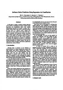
Figure 3.1: A sample rule tree for the KC1 dataset

35

With Clump, if the amount of entropy in a node exceeds a threshold value, a patch is created to reduce the intra-node entropy. Like Ripple Down Rule trees, the clusters made by Clump are also human maintainable. Figure 3.1 shows a sample rule tree generated by Clump. Clump differs from standard clusterers. Most clustering algorithms group rows based on the Euclidean distance between two rows or cluster centroids [3, 31, 51, 54]. This Euclidean distance (Equation 3.1) is determined by the combined absolute value of the delta between the two rows or the row and the centroid. v u u t

k

∑ (|row1[attributex ]2 − row2[attributex ]2|)

(3.1)

x=0

Clump accomplishes its clustering, not by Euclidean distance, but by how relevant a particular feature is in splitting the data. The exact equations used to determine the relevancy of a give attribute are shown in §3.2.1 Equation 3.2 - Equation 3.5. Grouping data by relevancy accomplishes much the same as grouping data by Euclidean distance. It provides several benefits as well. There is an explanation as to why a particular instance belongs to a particular cluster. Also, the standard n2 runtime of clustering algorithms is avoided because decisions made in generating the tree are made in respect to each row as its being examined, not by every row as each row is being examined. One goal of Clump is to create rule trees that are maintainable. The maintenance can be accomplished in two ways. First, if a rule tree is small enough, a human to look at the tree, and remember most if not all of it by recall. This allows the human to notice additions/subtractions that could be made to the tree by utilizing domain specific knowledge. Second, a tree can be built during initial training, and while being used with real-time data, can be patched to adapt to the changing data. A second goal of Clump is to form the nearest neighbor structure from the data in linear or low order polynomial time. Rule trees offer a significant advantage to frequency count learners such as Naive Bayes: Rule trees offer not just answers, they offer explanation. 36

Unlike Ripple Down Rules, Clump is not used for classification, but for clustering. Clump is used to find the structure within the data while avoiding the standard O(n2 ) clustering algorithms. While testing, Naive Bayes is used to do the classifying once the data has been limited by Clump as a clusterer.

3.2

The Design of Clump

Clump is a rule based decision tree clusterer. At its core, it is a binary tree with nodes that can have 0 − 2 children. Each node consists of a rule, its true and false conditions (if any), and a collection of training data that has reached that node. When testing, a testing example travels down the tree until it reaches a point where there are no children nodes for it to follow. The data that stored in that node is then passed to a naive bayes classifier for final classification. Most clustering algorithms use the nearest neighbor calculation to determine which cluster a record belongs to. This record by record comparison takes O(n2 ) comparisons, each record must be compared against every other record to minimize the dissimilarity. Clump creates it’s clusters, not by minimum dissimilarity, but by grouping records with similar attributes. Grouping by similar attributes leads to decreased run-times. Frequency counts can be gathered, and cached, which leads to decreased run-times. Frequency counts can be used to determine which attribute value pair to split on because of the types of rules created by Clump. When training, Clump produces greedy rules, adding one attribute to the rule at each level of the tree. Clump performs local feature subset selection as it creates the rules, only considering attributes that have not been considered further up the tree. The most important feature, determined by the reduction in entropy, is chosen for the splitting criteria at each branch of the tree. When choosing the splitting criteria, the standard entropy calculation is not used. The entropy is determined by the frequency of the different classes represented in the training rows at each branch of the tree, relative to the overall frequency of each class. This allows some features that might only

37

be important under specific circumstances to be used when needed, and ignored in the other parts of the tree.

3.2.1

Training

Training, like most tree building algorithms is a recursive process. Initially, a root node is made and populated with the entire training set. The default class is also set to the majority class. This root node is then passed to the training function. The training function looks at the data in the node, and if there are ≤ 15 rows in the data, training terminates. If there are ≥ 15 rows in the data, an optimal splitting criteria is chosen. Two resultant nodes are created and added as children of the generating node. All data from the generating node that satisfies the optimal splitting criteria is added to the true child node, and all that does not is added to the false child node. The process then recurses until all nodes are created. The optimal splitting criteria is used to create the rule, and split the data into two groups: the data that satisfies the splitting criteria, and the data that does not satisfy the splitting criteria. Each rule created is conditional on the node’s parent’s rule.

3.2.1.1

Scoring Function

When choosing the optimal splitting criteria, all possible splitting criteria for both positive and negative classes at a node are explored. Each possible split receives a score based on the relative frequency of the positive and negative records as described in Equation 3.2 - Equation 3.5.

Ptrue =

Ftrue | v Ftrue

(3.2)

Pf alse =

Ff alse | v Ff alse

(3.3)

38

function Training(data) if(numRows == 0 || depth >= 15) exit; for(row in data) for(column in columns) min(column) columnWidth = max(column) − 3 − min(column) row[column].value = row[column].value columnWidth

choices = GetColumnWeights(data) maxChoice = max(choices); rule = CreateRule(maxChoice, data) return rule rule.true = Training(data | rule) rule.false = Training(data | !rule)

function CreateRule(choice, data) rule.function = choice rule.true = Training(data | choice) rule.false = Training(data | !choice) return rule

function GetColumnWeights(data) for(column in columns) for(bin in column) trueData = data | column.value = bin && data.class = true falseData = data | column.value = bin && data.class = false column.bin.weight = max( data | trueData.size data.class = true , f alseData.size data | data.class = f alse )

Figure 3.2: Pseudo code of the Clump Training process

39

Scoretrue =

Ptrue Ptrue + Pf alse

(3.4)

Score f alse =

Pf alse Pture + Pf alse

(3.5)

This scoring function removes the bias to choose classes with more overall support. This is done by normalizing the frequency of the class at a node by representing it as the percentage of all examples of class C present in the node. Comparing the relative frequency of the true versus the false nodes this way can show the presence or lack thereof of a bias towards one class versus the other.

3.2.1.2

Dependent/Independent Attributes

An attribute is independent [34] when the attribute value is disassociated from the class attribute. A dependent [34] attribute is when the attribute value is considered in conjunction with the class attribute. Most clustering algorithms [31,64,66,71] consider independent attributes, building clusters without considering the classes of the intra node instances. Clump builds its clusters by reducing intra node entropy. To accomplish this, an attribute value is chosen according to the process is §3.2.1.1. The attribute chosen will create two sub clusters each containing a higher frequency of one class than the combine parent cluster.

3.2.1.3

Boosting

Traditional boosting [58] is where the training instances that fail classification with one learner will be used to train a second learner. This process can be repeated many times, resulting in a chain of learners that can then be pooled for final classification. This is commonly referred to as “toilet learning,” as each successive learner is trained off of the dregs of the learner before it. Clump represents boosting by creating sub clusters of data when the data added to a cluster becomes too 40

function Testing(data) chunks = split(data) for(chunk in chunks set) for(row in chunk) gatheredData += GatherData(tree, row) nb = NaiveBayes(gatheredData) return nb(data) Figure 3.3: Pseudo code of the Clump Testing process diverse. Clump creates sub clusters that have a lesser combined mean degree of diversity within each other than within the parent cluster.

3.2.1.3.1

AdaBoost Clump shows some similarity to a boosting algorithm called AdaBoost

[23]. AdaBoost repeatedly iterates over the model, modifying distributions at each iteration to reduce the overall error on the training set. Internally, a simple classification algorithm is used. This algorithm, called the WeakLearn, must only consistently perform better than random guessing. Through many iterations, the error rate is reduced. The main difference between Clump and AdaBoost is the branching associated with Clump. Data is split at each decision, meaning Clump is working with less and less data at each branch.

3.2.2

Testing

When testing, one or more testing rows are combined to form a chunk of rows. Each row from a chunk is sent down the tree, and the data stored at the node where the row stops is combined. The row of data continues its travel down the tree, following the true and false branches as necessary until a leaf node is reached. The row then travels back up the tree until the last satisfied rule is reached. While combining the data, any duplicates are ignored2 . This combined training data is then passed to a Naive Bayes classifier. Each row in the testing chunk is then passed to the Naive 2A

duplicate is defined as a specific training instance, not the combination of attribute values

41

Runtime while Training Testing

Naive Bayes O(nk) O(mk)

Ridor O(nk ∗ log(kn) O(md)

Clump O(3nk ∗ log(kn)) O(mk) - O(mkd)

LWL O(n) O(mnk)

j48/C4.5 O(nk ∗ log(n)) O(m ∗ log(m))

RIPPER O(2nk ∗ log(kn)) Unlisted

OneR O(kn) O(1)

Figure 3.4: Runtime Complexity of Clump, Naive Bayes [36], Ridor, OneR [6], LWL [22], j48/C4.5 [7], and RIPPER [24] on a dataset with n training cases, m testing cases, d tree depth, and k attributes.

Bayes classifier for final classification. When gathering the data for the Naive Bayes classifier, each node is marked if the data should be used in classification. Each node will only be included once, even if multiple chunk rows fall to that node. Some data may be included more than once because if a row stops at a parent node and another row stops at a child node, the data in the child node is also included in the parent node. After all the nodes have been marked, the tree is iterated through a second time to gather the final training dataset.

3.2.3

Discretization

The rules are based on which bin the discretized attributes belong in. Rather than rules reading: “If attributex < value then ...”, the rules for Clump read: “If attributex is in bin x then ...”. Discretizing is done using equal width discretization [69]. Each attribute range is broken up into three different bins, with each bin having the same width, or the same distance between the minimum and maximum values for the bin. Three bins were chosen by experimental testing. Equal width discretization was chosen above other options such as Equal frequency discretization [4] and Fayyad & Irani’s MDL discretizer [17]. These other options were tried, and showed no noticeable performance improvement, while adding complexity to the algorithm.

42

Within-Company Raw Logging Ridor 2.56 2.52 jRip 2.45 2.53 Clump 3 3

Cross-Company Raw Logging 3.34 3.27 4.06 4.17 3 2 Table 3.1: Number of rules

Within-Company Raw Logging Ridor 6.1 6.4 jRip 3.1 2.9 Clump 3 3

Cross-Company Raw Logging 10.9 17.3 13.4 13.4 3 2 Table 3.2: Number of conditions

3.2.4

Runtime Complexity

The theoretical runtime of Clump while training is O((3kn + k) ∗ logkn ) where k is the number of columns in the dataset, and n is the number of rows. When training, each record is examined to determine which bin it belongs to (O(1kn)). To create the bins, the minimum and maximum values of each attribute must be found (O(1kn)). Next, a Naive Bayes classification table is built with a runtime cost of O(1kn). If the data requires, a patch is created by examining the frequency count tables for an attribute value pair that will reduce the mixuped-ness of the data. This is repeated at each level of the tree with the amount of data, in both the row count and the column count, decreasing at each level of the tree. With the current built-in classifier of Naive Bayes, the theoretical maximum runtime for testing is O(nkd), where d is the depth of the tree. This worst case scenario occurs when all the data is contained in a single cluster. The current maximum depth is limited to 15 levels. The theoretical minimum runtime for testing is O( nk d ). This best case scenario occurs when the data is evenly distributed across n-dimensional space, causing each node in the tree to contain an equal number of rows.

43

3.2.5

Rule Complexity

The number of rules for Clump, Ridor, and Ripper are shown in Table 3.1. The size of the rule tree generated by Clump is similar to the number of rules in Ridor and Ripper. When looking at within company tests, Clump has, on average, an extra 0.5 rules. In the Cross Company tests though, Clump generates the between same number of rules to twice the number of rules in Ridor and Ripper. Typically because of the increased number of training instance, Cross Company tests result in more complex models being learned. Clump, on the other hand, has the same theory complexity when looking at Cross Company as Within Company. The difference in the complexity of these three algorithms’ models is apparent in Table 3.2. Table 3.2 shows not just the number of rules generated by each algorithms, but the number of attribute value comparisons made in each learned model. In the Within Company tests, Ripper and Clump have approximately the same complexity: 1 comparison per rule. Ridor on the other hand has 2 comparisons per rule. These numbers start to really climb when looking at the Cross Company tests. Ripper and Ridor have between 3 and 5 comparisons per rule, while Clump still remains at 1 comparison per rule. The simple theories learned by Clump help to provide a clear explanation for the theories learned.

3.3

Summary

This chapter detailed a new algorithm that was a merger between a clusterer and a classifier called Clump. The clustering aspect of Clump differs from other clustering algorithms by creating its clusters with a decision tree. Clump relies on individual attribute values, and not a standard Euclidean distance. The classification aspect of Clump uses Naive Bayes. Clump performs similarly to Naive Bayes, but offers an advantage over Naive Bayes by providing an explanation for its decisions by way of the decision trees. Clump also has a higher probability of detection than the other classifiers. These results are detailed in Chapter 5. The next chapter details the experimental design, the pre-processing algorithms used, and the 44

methods used for analysis.

45

Chapter 4 Laboratory Studies This chapter details the experiments that will be conducted. Without proper experimentation, it is impossible to come to a defensible conclusion. Below I will describe the experimentation procedures I will use, the datasets the experiments will be applied to, and how the results will be evaluated. Just as different classification algorithms will be explored, I will also look into the usage of several pre-processing algorithms. The goal of these experiments is to evaluate how locality impacts classification performance for software defect prediction. First, the experimental procedure and datasets are explained. Next, the algorithms are individually analyzed, with special attention being paid to Locally Weighed Naive Bayes. Third, relevancy filtering is explored by applying the Burak filter. Finally, the original experiments, augmented with various clustering algorithms, are re-run. The results of these experiments will be explored in Chapter 5.

46

for data in $datasets; do preProcess $data > processed.arff for((r=1;r results.dat done done done done Figure 4.1: The pseudo code to run an experiment with Ourmine [27]

4.1

Experimental Design

Below, I will explain the experimental procedures I will follow, what types of data are collected, and how it will be evaluated. The format of the data, and an explanation of the attributes within the data will be detailed. I will explore the classifiers mentioned in Chapter 2 by applying them to software defect prediction. I will explore the data in two separate ways: • Within Company • Cross Company I will also apply various relevancy filtering and clustering algorithms to the data, and observe the differences between applying the pre-processed data versus the original data to the classification algorithms.

4.1.1

Testing Framework

Experimenting is accomplished using the Ourmine [27] framework developed at West Virginia University. This framework allows for easy generation of testing and training datasets, as well as 47

statistical processing. The framework is a collection of bash scripts that have a standardized format for the various types of input and output. The classifiers each take the relative path to a training and testing dataset. After training the classifier, the testing results are outputted to be collected by the statistics part of Ourmine. The output is in the form of a ”got-want” result for each testing instance. ”Want” is class of the testing instance, and ”got” is the classification returned by the classifier.

4.1.2

Datasets

The datasets used come from the NASA/MDP and the SoftLab data sets1 from the Promise Data Repository [57]. The NASA/MDP datasets used are: CM1, KC1, KC2, KC3, MC2, MW1, and PC1. These datasets were chosen for examination because they represent a wide variety of projects. A frequently posed objection to using the NASA datasets in a Cross-Company examination is that all the datasets are written for a single organization, and do not represent a proper sampling of software styles and development procedures. When writing about software defect datasets from NASA, Zimmermann et al. states: For their study Turhan et al. [64] analyzed 12 NASA projects (mostly in C++) which they considered cross-company because they were all developed by contractors under the umbrella of NASA. However, all projects had to follow stringent ISO-9001 industrial practices imposed by NASA, so it is unclear to what extent the data can be actually considered cross-company. [72] Menzies et al. retorts that: ”NASA is a much more diverse organization than is commonly appreciated. NASA software is written by layers of contractors working for different companies around the 1 The

datasets can be obtained at http://promisedata.org

48

nation. Arguing that all ISO-compliant organizations are the same is like saying that a CMM level3 weapons manufacturer is writing the same software as a CMM level3 finance company.” [44] The NASA datasets represent projects such as flight software, storage management, video guidance systems, and an experiment framework [64]. Also, the majority of the data used in the NASA datasets is from ground control software, not flight control. As such, it is not as constrained during its development. Menzies et al. shows empirical evidence that the NASA datasets represent truly different development practices and methodologies. The SoftLab datasets are AR3, AR4, and AR5. These datasets were chosen for examination because they represent a different spectrum of products, decreasing the similarity of the tested datasets. While the NASA datasets are usually large, and highly critical systems, the SoftLab datasets represent the embedded systems in some Turkish white goods. The embedded systems control three separate appliances including a washing machine. These datasets differ from the NASA/MDP datasets in their severity, scope, and purpose. The files have been modified from their original form to allow them to be used in cross company experiments2 . They have been modified to unify the columns used, and their orderings. The data is stored in the arff format for easy integration with the WEKA experimenter [29]. Figure 4.2 shows the attributes present in each dataset. Attributes marked with a ”X” are used in both the Within Company and Cross Company experiments. The attributes marked with a ”W” are only used in the within company experiments. These datasets will be used in all further studies unless noted otherwise.

4.1.3

Dataset Format

The data used for training and testing is stored in the arff format. This format was chosen to insure compatibility with past and future experiments. This is the format used by the Modeling 2 Cross

company experiments use n − 1 of n datasets for training, and the nth for testing

49

Attribute Lines of Code (lOCode) Blank Lines of Code Lines of Comments LoC + Lines of Comments Executable Lines of Code Unique Operands Unique Operators Total Operands Total Operators Halstead Vocabulary Halstead Length Halstead Volume Halstead Level Halstead Difficulty Halstead Effort Halstead Error Halstead Time Branch Count Cyclomatic Complexity Cyclomatic Density Design Complexity Decision Count Call Pairs Condition Count Multiple Condition Count Decision Density Design Density Normalized Cylc. Complex. Format Parameters Number of Lines Percent Comments Modified Condition Count Maintenance Severity Node Count Edge Count Essential Complexity Essential Density

AR3 X X X X X X X X X X X X X X X X X X X X X W W W W W W W W

AR4 AR5 CM1 KC1 X X X X X X X X X X X X X X X X X X X X X X X X X X X X X X X X X X X X X X X X X X X X X X X X X X X X X X X X X X X X X X X X X X X X X X X X X X X X X X X X X X X X W W W W W W W W W W W W W W W W

KC2 KC3 MC2 MW1 PC1 X X X X X X X X X X X X X X X X X X X X X X X X X X X X X X X X X X X X X X X X X X X X X X X X X X X X X X X X X X X X X X X X X X X X X X X X X X X X X X X X X X X X X X X X X X X X X X X X X X X X X X X X X W W W W W W W W W W W W W W W W W W W W W W W W W W W W W W W W W W W W W W W W W W W W W W W W W W W W W W W W W W W W W W W W

Figure 4.2: Attributes used in datasets for LWL and Classifier experiments

50

@relation KC1 @attribute loc numeric @attribute v(g) numeric @attribute ev(g) numeric @attribute iv(g) numeric @attribute v numeric @attribute l numeric @attribute d numeric @attribute i numeric @attribute e numeric @attribute b numeric @attribute t numeric @attribute lOCode numeric @attribute lOComment numeric @attribute locCodeAndComment numeric @attribute defects {false,true} @data 4.62497,3.04452,2.07944,2.30259,7.43822,-3.21888,3.32251,4.11578,10.7607,-0.562119,7.87035,4.36945,1.38629,0.693147,true 2.83321,0,0,0,5.65351,-2.30259,2.32337,3.3297,7.97731,-2.30259,5.08692,2.83321,2.89037,-11.5129,false 2.19722,2.07944,4.45377,-11.5129,1.60944,1.79176,1.51951,2.93386,5.97361,-3.50656,1.60944,3.09104,1.09861,2.83321,false 1.79176,0,0,0,3.11174,-0.693147,0.693147,2.41859,3.80488,-4.60517,0.916291,-11.5129,-11.5129,-11.5129,false 4.06044,4.85203,7.54602,-11.5129,1.94591,-11.5129,2.89646,4.64938,10.4427,-0.462035,1.38629,5.73979,1.60944,4.29046,false -11.5129,-11.5129,-11.5129,-11.5129,0,-11.5129,-11.5129,-11.5129,-11.5129,-11.5129,0,0,0,0,false 1.38629,0,0,0,2.07944,-0.400478,0.405465,1.67335,2.48491,-11.5129,-0.400478,0.693147,-11.5129,-11.5129,false 1.94591,0.693147,0,0.693147,4.44394,-2.30259,2.3155,2.12942,6.75895,-3.50656,3.86849,1.94591,-11.5129,-11.5129,false

Figure 4.3: A sample arff file for the partial KC1 dataset Intelligence Lab at West Virginia University. The format consists of the following: • The name of the dataset. • A list of the attributes. • A comma separated list of the data. • Any comments such as copy write information, details about the data collection process, and descriptions of any abnormalities. Each attribute consists of a name and its type. The type is either the word numeric, signifying that the data consists of a continuous range of numbers, or a list of discrete values, separated by commas and wrapped with braces. The last attribute is used as the class attribute. Comments can be included in any place in the document by precluding the comment by a percent sign (%). Each dataset has the same attributes so that the 10 datasets could all be used in Cross Company Examination. To accomplish this, many attributes had to be removed from each dataset. The 51

datasets used originally had upwards of 39 separate attributes, but only the 18 attributes and class attribute described below were shared between all 10 datasets. These attributes used are a mixture of the McCabe Code Metrics [67], Halstead Code Metrics [61], and static Line of Code Metrics. Each instance represents one module from the original source code. The code statistics are compiled using various code metric collection tools such as the Prest Metrics Extraction and Analysis Tool3 [65] The attributes used are as follows: • Halstead Code Metrics: – Program Volume: The information contents of the module. – Program Level: The inverse of the error proneness. – Difficulty Level: The error proneness of a module. – n1: Unique Operators. – n2: Unique Operands. – N1: Total Operators. – N2: Total Operands. – Effort To Implement: Program Volume ∗ Difficulty Level. 2

– Number of Delivered Bugs: – Time to Implement:

(Program Volume∗Difficulty Level) 3 3000

Program Volume∗Difficulty Level 18

.

seconds to implement.

– Intelligent Content: The complexity of the underlying algorithms as expressed in any language. • McCabe Code Metrics: – v(g): Cyclomatic Complexity. 3 This

tool is used to extract the metrics for AR3, AR4, and AR5.

52

– ev(g): Essential Complexity. • Line of Code Metrics: – Lines: The total number of lines in the module. – Branch Count: The number of branching decisions in a module. Ax example would be for loops, if/then/else statements, etcetera. – Lines of Code: The number of lines in the module that contain executable code or whitespace. – lOComment: The number of lines in the module that contain comment code. – locCodeAndComment: The number of lines in the module that contain comments or executable code. • Defects: If a module was defective or non-defective.

4.1.4

Experimental Method

Each classifier will be run many times to insure a significant number of trials are run. For the Within Company experiments, each trial will start by randomizing the datasets to eliminate any artifacts caused by data ordering. Next, the dataset will be broken into n separate parts, each of an equal size. In series, one is used as the testing dataset, and the remainder are used as the training dataset. This is referred to as a n-way cross validation [28]. N-way cross validation is important to the experimental procedure because it verifies that the classification algorithms are able to generalize the knowledge learned, and perform well on previously unseen data. I ran 5 random orderings of the datasets, and a 5-way cross validation. This will equate to 25 trials per dataset. In Cross Company experiments, each trial will again start by randomizing all datasets. In series, each dataset is a testing dataset, and the remaining datasets are combined to form the training 53

Actual \ Predicted False True False a b True c d Figure 4.4: An example confusion matrix

dataset. When performing a Cross Company experiment, it is not possible to do the standard n-way validation of splitting the data into n equal sized bins because no part of the testing dataset can exist in the training dataset, or the purpose of Cross Company would be violated. The Cross Company experiments are also subjected to 5 random orderings of the datasets. The random orderings, coupled with the modified n-way cross validation will result in 5 ∗ N trials, where N is equal to the number of datasets being explored.

4.1.5

Evaluation of Results

The output of all the trials will be combined to form the final results. This information is then used to generate a ”abcd” stats(Figure 4.4), or a confusion matrix [39], for each trial. One item of importance, as it deviates from the ”normal” method of benchmarking classifiers, I will only report statistics on the defective modules. The correctly identified non-defective modules will be ignored. From the gathered ”abcd” stats, two other statistics are generated: The Probability of Detection(PD - Equation 4.1), and the Probability of False Detection(PF - Equation 4.2).

PD =

D B+D

(4.1)

PF =

C C+A

(4.2)

These are the statistics used for further examination. The combined set of Probability of Detection and Probability of False alarm rate statistics for each trial is then ranked according to

54

a Mann-Whitney-Wilcoxin [15] U test. With the Mann-Whitney-Wilcoxon ranks, you can determine, within a certain percentage of confidence, whether two methods are equivalent, if one method out-performs the other method. I will report Mann-Whitney-Wilcoxon ranks within a 95% confidence interval unless stated otherwise. I will also show quartile charts of the Probability of Detection and Probability of False alarm rates. The quartile charts will show the 2nd quartile, the median value, and the 3rd quartile. I will compare the classifiers described in Chapter 2 and Chapter 3 to each-other, showing their relative performance to the other classifiers. I will also explore the application of K-Means and Greedy Agglomerative Clustering, comparing the classifier with and without the clusterer being applied. These various experiments will paint a picture about the usefulness of locality, both in the classifier and in the application of the clusterers, being applied to software defect prediction.

4.2

Various Classification Algorithms

Two groups of classification algorithms are explored. The first group are locality based classification algorithms such as LWL, Ridor, Clump, and RIPPER. The second group are non-locality based learners such as C4.5, OneR, and Naive Bayes. I will explore the difference in performance of the locality based and non-locality based classifiers. In these results, I will also compare the difference in using Within Company data versus Cross Company data. Finally, I will explore an effect demonstrated by Turhan [64] where logging the numerical data helps improve the classification performance. Each of the classifiers have various configuration options described in Table 4.1. Table 4.1 also details the options which were chosen for experimentation. Multiple versions of LWL were tried, using a range of K values.

55

Naive Bayes can use a normal distribution, a Kernel estimation, or supervised discretization to discretize numeric attributes. We examine the normal distribution to accomplish discretization. C4.5 can set a minimum number of instances per leaf node and set the confidence threshold for pruning. We examine a minimum of 2 instances per leaf node and a confidence threshold of 0.25. OneR can set the minimum number of instances per rule. We examine a minimum of 6 instances per rule. LWL can set the kernel shape to use for weighting and the number of nearest neighbors to include in the kernel shape. We examine a linear kernel, and a variety of nearest neighbors. This is detailed in §4.2.1. RIPPER can choose the quantity of data to use for pruning, the minimum number of instances per rule, and the number of optimization runs to perform. We examine the default values of 31 of the data for pruning, a minimum of 2 instances per rule, and 2 optimization runs to reduce error. Ridor can choose the quantity of data to use for pruning and the minimum number of instances per rule. We examine the default values of 31 of the data for pruning and a minimum of 2 instances per rule. Clump can choose the the minimum number of instances per node and the threshold of mixedupedness until a node attempts to split. We examine a minimum of 5 instances per node, and a threshold of 5 non-majority class instances. These values were arrived at via experimentation. Table 4.1: Configuration Options for the Classification Algorithms

56

Learner Rank min LWL-5 1 0.0 LWL-10 1 0.0 LWL-25 2 0.0 LWL-50 3 0.0 LWL-100 4 0.0

Learner Rank min LWL-100 1 0.0 LWL-25 1 0.0 LWL-10 1 0.0 LWL-5 1 0.0 LWL-50 1 0.0

q1 0.0 0.0 0.0 0.0 0.0

PD Quartile median q3 50.0 88.9 50.0 90.0 40.0 84.6 25.0 85.7 0.0 50.0

max Quartile u 100.0 u 100.0 u 100.0 u 100.0 u 100.0

q1 0.0 0.0 0.0 0.0 0.0

PF Quartile median q3 0.0 11.1 3.2 7.1 3.3 7.1 3.3 6.9 3.3 9.7

max 41.4 32.1 24.1 24.1 34.5

Quartile u u u u u

Table 4.2: Various K values for LWL on UCI dataset Fish Catch.

Learner Rank min LWL-10 1 0.0 LWL-5 1 10.0 LWL-25 1 0.0 LWL-50 2 0.0 LWL-100 3 0.0

PD Quartile q1 median q3 20.0 47.1 60.0 25.0 45.5 60.0 25.0 44.4 60.0 12.5 40.0 58.3 0.0 30.0 53.8

Learner Rank min LWL-100 1 0.0 LWL-50 2 0.0 LWL-5 2 0.0 LWL-25 2 0.0 LWL-10 3 0.0

PF Quartile q1 median q3 0.0 3.2 8.9 1.0 3.2 8.1 1.1 3.3 9.3 1.1 3.3 8.2 1.1 4.1 9.9

max Quartile u 100.0 u 100.0 u 100.0 u 100.0 u 100.0

max 39.1 36.8 25.0 27.8 24.2

Quartile u u u u u

Table 4.3: Various K values for LWL on UCI dataset Housing.

57

Learner Rank min LWL-25 1 0.0 LWL-50 2 0.0 LWL-10 3 0.0 LWL-5 4 0.0 LWL-100 4 0.0

Learner Rank min LWL-100 1 0.0 LWL-25 1 0.0 LWL-50 2 0.0 LWL-10 3 0.0 LWL-5 4 0.0

q1 0.0 0.0 0.0 0.0 0.0

PD Quartile median q3 66.7 83.3 50.0 81.8 50.0 66.7 40.0 62.5 14.3 72.7

max Quartile u 100.0 u 100.0 u 100.0 u 100.0 u 100.0

q1 0.0 0.0 0.0 0.0 0.0

PF Quartile median q3 2.3 9.1 2.3 5.0 2.4 6.8 4.3 8.3 4.4 9.5

max 27.5 16.7 20.0 21.4 25.6

Quartile u u u u u

Table 4.4: Various K values for LWL on UCI dataset Body Fat.

Learner Rank min LWL-50 2 0.0 LWL-25 2 10.0 LWL-100 1 0.0 LWL-5 3 0.0 LWL-10 2 0.0

Learner Rank min LWL-100 1 0.0 LWL-50 2 1.2 LWL-5 3 2.4 LWL-25 2 2.4 LWL-10 2 0.0

q1 28.6 25.0 25.0 20.0 25.0

PD Quartile median q3 50.0 96.3 50.0 95.1 50.0 97.6 50.0 94.2 50.0 94.3

PF Quartile q1 median q3 1.2 5.7 72.7 3.6 8.2 70.0 4.9 9.5 71.4 4.9 9.8 71.4 5.0 10.5 75.0

max Quartile u 98.8 u 97.6 u 100.0 u 97.6 u 100.0

max Quartile 100.0 u u 100.0 u 100.0 u 90.0 u 100.0

Table 4.5: Various K values for LWL on NASA dataset KC3.

58

4.2.1

A Close Look at Locally Weighted Naive Bayes

Locally Weighed Naive Bayes, also called Locally Weighted Learning, is a K nearest neighbors algorithm. When using Locally Weighted Learning on the UCI datasets [1], it was noted that the value of K strongly impacted the performance of LWL. I chose to explore K values of 5, 10, 25, 50, and 100. It was also noted that the K value chosen was dataset specific, as shown in Table 4.2, Table 4.3 and Table 4.4. Note that the optimal K value in the three examples is between 5 and 25. By tuning the K value, historically, the performance of LWL has statistically improved. When looking at the NASA and SoftLab software defect prediction datasets, I show that across 9 of the 10 datasets4 , all values of K performed statistically the same. Although performances look varied, the Mann Whitney Wilcoxin Rank of each learner across the 9 datasets is identical at both the 95% and 99% confidence intervals. The results for the 9 identical datasets are shown at the end of this chapter in Table 4.7 - Table 4.15. The one outlier, NASA’s KC3 dataset is shown in Table 4.5. This similarity will be looked into further in Chapter 5.

4.3

Pre-Processing by Relevancy Filtering

I will also explore the Burak Filter as a relevancy filter. The Burak Filter is a modified K Nearest Neighbor algorithm used to filter the training data to only include the training instances which are similar to the testing instances. I will compare the performance of each algorithms listed in §2.4.1, §2.4.2, and Chapter 3 against the algorithm augmented by the Burak Filter. With this, I hope to show that the Burak Filter, currently the ”gold standard” in relevancy filtering, does not beneficially impact the performance of the clustering algorithms listed above. 4 The

exception is KC3

59

4.3.1

A Difference in Results

Turhan et al. [64] explored the effect of the Burak Filter on software defect prediction in their 2009 paper ”On the relative value of cross-company and within-company data for defect prediction”. Their results differ from the results that are presented in Chapter 5. In this section, I will discuss their results for Within Company, Cross Company and Nearest Neighbor augmented Cross Company over the 7 NASA datasets listed in §4.1.2.

Dataset CM1 KC1 KC2 KC3 MC2 MW1 PC1

Turhan [64] WC NN 2nd 1st 1st 2nd 1st 2nd 1st 2nd 1st 2nd nd 2 1st 2nd 1st

Reproduction WC NN 2nd 1st 1st 2nd 1st 2nd 2nd 1st 2nd 1st st 1 2nd 2nd 1st

(a) PD Ranks

Dataset CM1 KC1 KC2 KC3 MC2 MW1 PC1

Turhan [64] WC NN 1st 2nd 2nd 1st 2nd 1st 2nd 1st nd 2 1st 1st 2nd 1st 2nd

Reproduction WC NN st 1 2nd 2nd 1st 2nd 1st 2nd 1st nd 2 1st 1st 2nd 2nd 1st

(b) PF Ranks

Table 4.6: Burak Reproduction Results Although I were unable to reproduce the Cross Company results showing in Turhan’s paper [64], I were able to duplicate the pattern of their results for Within Company and Nearest Neighbor in the majority of cases. Turhan et al. report that the Cross Company PD’s reported in their paper were the highest reported as of the publication of their paper, and to our knowledge those results 60

have not been duplicated. Table 4.6 shows Burak’s original results and our reproduction of those. The ranks shown are the numerical orderings of the median PD and PF values. In our reproduction, PD and PF’s for CM1, KC1, and KC2 followed the pattern displayed by Turhan. For KC3, MC2, and MW1, the PF matched the pattern. For PC1, the PD matched the pattern. The differences between our reproduction and Turhan’s results may be caused by many factors, such as: • The datasets used for our results have been modified to use both the NASA datasets and the SoftLab datasets in the Cross-Company experiments. • Differences in algorithm implementations. • Minor differences in statistics gathering. These results shown here are in contradiction to what will be shown in §5.2 and §5.1. The reason for this is in the statistics gathering. Turhan reported their results on both the defective and non-defective modules. I feel that only the records that involve the defective modules should be used for reporting on software defect prediction. This belief is because the defective modules are the modules I are attempting to identify. I also care about incorrectly classified non-defective modules, as they increase the cost of testing. In the remainder of this thesis, I will report results as described in §4.1.5.

4.4

Pre-Processing by Clustering

I will explore clustering algorithms by applying K-Means and Greedy Agglomerative Clustering to the classifiers listed above. The performance of these clustering algorithms and the Burak Filter are compared by applying them to the datasets in §4.1.25 and the locality based classifiers listed in §2.4.1, non-locality based classifiers in §2.4.26 , and Clump. 5 AR3, 6 Local

AR4, AR5, CM1, KC1, KC2, KC3, MC2, MW1 classifiers: LWL, Ridor, RIPPER. Non-Local Classifiers: C4.5, Naive Bayes, OneR

61

With these experiments, I hope to show that locality by clustering does not beneficially impact the performance of the classification algorithms.

4.5

Summary

In this chapter, I explained the the data being used for experimentation including its format [29], sources [57], and its attributes. I also covered the experimental methods. The layout of the experiments, and the evaluation criteria were detailed. The results are displayed using quartile charts, and will include the Mann-Whitney-Wilcoxin U-Test ranks. Finally, the different experiments performed were detailed. These include: • A comparison of locality based and non-locality based classifiers. This will show the effects of locality during classification. • A comparison of the application of a relevancy filter versus not applying the filter. This will show the effects of locality during training. • A comparison of various clustering algorithms versus no pre-processing. This will show the effects of locality during the instance selection process. I will demonstrate this process by using the clustering algorithm to select the local training data for each testing instance. I will then retrain the classifier with this new local training data. Many results were observed in the process of running the above experiments, and the next chapter will present these results.

62

Learner Rank min LWL-25 1 0.0 LWL-5 1 0.0 LWL-50 1 0.0 LWL-100 1 0.0 LWL-10 1 0.0

Learner Rank min LWL-50 1 1.2 LWL-100 1 1.2 LWL-25 1 1.2 LWL-10 1 3.5 LWL-5 1 3.4

q1 16.7 11.8 12.5 10.0 16.7

PD Quartile median q3 66.7 91.4 40.0 90.0 33.3 94.3 33.3 95.1 33.3 92.4

max 98.8 96.6 98.8 98.8 96.5

q1 5.4 4.5 7.0 7.3 7.6

PF Quartile median q3 11.1 83.3 12.2 85.7 12.2 83.3 15.6 82.4 15.6 87.5

max Quartile u 100.0 u 100.0 u 100.0 u 100.0 u 100.0

Quartile

u u

u u u

Table 4.7: Various K values for LWL on NASA dataset CM1.

Learner Rank min LWL-10 1 27.9 LWL-5 1 26.2 LWL-25 1 21.3 LWL-50 1 13.2 LWL-100 1 10.3

Learner Rank min LWL-100 1 2.0 LWL-50 1 2.6 LWL-10 1 5.6 LWL-25 1 4.5 LWL-5 1 5.0

PD Quartile median q3 55.0 91.7 48.3 91.5 45.2 92.8 40.0 93.9 36.7 95.6

max 94.4 95.0 95.5 97.4 98.0

Quartile

PF Quartile q1 median q3 4.2 5.8 75.0 5.9 9.0 69.6 8.2 10.6 60.5 7.0 11.0 63.7 8.1 12.0 62.7

max 89.7 86.8 72.1 78.7 73.8

Quartile

q1 39.1 36.4 33.9 27.5 24.6

u

u u u u

u u u u u

Table 4.8: Various K values for LWL on NASA dataset KC1.

63

Learner Rank min LWL-25 1 30.4 LWL-10 1 32.0 LWL-50 1 27.3 LWL-5 1 28.0 LWL-100 1 22.7

q1 47.1 50.0 47.1 50.0 41.2

PD Quartile median q3 75.0 89.0 75.0 89.2 72.7 91.4 68.8 88.8 56.2 93.2

max 96.3 92.9 95.1 93.9 98.8

Quartile

Learner Rank min LWL-100 1 1.2 LWL-10 1 7.1 LWL-50 1 4.9 LWL-5 1 6.1 LWL-25 1 3.7

PF Quartile q1 median q3 6.2 12.8 56.5 10.3 15.5 50.0 8.5 15.7 50.0 10.1 16.7 50.0 9.4 17.9 50.0

max 77.3 68.0 72.7 72.0 69.6

Quartile

u u u u u

u u u u u

Table 4.9: Various K values for LWL on NASA dataset KC2.

Learner Rank min LWL-100 1 0.0 LWL-10 1 9.1 LWL-50 1 0.0 LWL-5 1 16.7 LWL-25 1 9.1

q1 30.8 30.8 35.7 38.5 36.4

PD Quartile median q3 83.3 87.5 63.6 77.3 62.5 86.4 62.5 75.0 52.4 81.0

Learner Rank min LWL-100 1 0.0 LWL-50 1 0.0 LWL-10 1 13.0 LWL-5 1 9.5 LWL-25 1 4.2

q1 10.5 11.1 21.1 23.8 18.2

PF Quartile median q3 16.7 63.6 23.8 62.5 36.4 61.5 36.4 60.0 42.1 63.6

max Quartile 100.0 87.0 100.0 90.5 95.8

max Quartile u 100.0 u 100.0 u 90.9 u 83.3 u 90.9

u u u u u

Table 4.10: Various K values for LWL on NASA dataset MC2.

64

Learner Rank min LWL-100 1 14.3 LWL-50 1 14.3 LWL-25 1 0.0 LWL-10 1 0.0 LWL-5 1 0.0

Learner Rank min LWL-100 1 1.3 LWL-25 1 1.3 LWL-10 1 2.6 LWL-5 1 1.4 LWL-50 1 1.3

q1 33.3 28.6 20.0 22.2 20.0

PD Quartile median q3 80.0 94.7 66.7 94.6 60.0 94.6 60.0 93.3 50.0 94.7

max 98.7 98.7 98.7 97.4 98.6

q1 4.2 5.4 5.4 4.2 5.3

PF Quartile median q3 10.1 66.7 12.0 75.0 12.7 71.4 13.3 77.8 14.1 66.7

max Quartile u 85.7 u 100.0 u 100.0 u 100.0 u 85.7

Quartile

u u u u u

Table 4.11: Various K values for LWL on NASA dataset MW1.

Learner Rank min LWL-50 1 7.7 LWL-100 1 5.3 LWL-5 1 0.0 LWL-10 1 13.3 LWL-25 1 7.7

Learner Rank min LWL-100 1 0.5 LWL-50 1 1.0 LWL-10 1 0.5 LWL-5 1 2.0 LWL-25 1 1.0

q1 30.8 21.4 31.2 30.0 30.0

PD Quartile median q3 60.0 97.1 60.0 98.5 60.0 96.0 53.3 96.2 50.0 96.7

PF Quartile q1 median q3 1.5 3.0 76.9 2.5 5.8 68.8 3.4 5.9 68.8 3.9 6.8 68.2 3.0 7.2 68.8

max 99.0 99.5 98.0 99.5 99.0

Quartile

u u u u u

max Quartile 94.7 u 92.3 u 86.7 u u 100.0 u 92.3

Table 4.12: Various K values for LWL on NASA dataset PC1.

65

Learner Rank min LWL-50 1 0.0 LWL-100 1 0.0 LWL-25 1 0.0 LWL-10 1 0.0 LWL-5 1 0.0

Learner Rank min LWL-100 1 0.0 LWL-25 1 0.0 LWL-50 1 0.0 LWL-10 1 0.0 LWL-5 1 0.0

q1 50.0 50.0 33.3 50.0 50.0

PD Quartile median q3 100.0 100.0 100.0 100.0 91.7 100.0 90.9 100.0 83.3 100.0

max Quartile 100.0 100.0 100.0 100.0 100.0

q1 0.0 0.0 0.0 0.0 0.0

PF Quartile median q3 0.0 18.2 0.0 33.3 0.0 18.2 9.1 18.2 9.1 33.3

max 100.0 100.0 100.0 100.0 100.0

u u u u u

Quartile u u u

u u

Table 4.13: Various K values for LWL on SoftLab dataset AR3.

Learner Rank min LWL-25 1 0.0 LWL-100 1 0.0 LWL-5 1 0.0 LWL-50 1 0.0 LWL-10 1 0.0

q1 33.3 50.0 33.3 40.0 33.3

PD Quartile median q3 75.0 88.9 75.0 88.2 68.4 85.7 66.7 88.2 66.7 85.7

Learner Rank min LWL-25 1 0.0 LWL-100 1 0.0 LWL-50 1 0.0 LWL-10 1 0.0 LWL-5 1 0.0

q1 11.1 11.1 11.1 12.5 12.5

PF Quartile median q3 22.2 50.0 25.0 50.0 25.0 50.0 27.8 60.0 31.2 66.7

max Quartile 100.0 100.0 100.0 100.0 100.0

max Quartile u 100.0 u 100.0 u 100.0 u 100.0 u 100.0

u u u u u

Table 4.14: Various K values for LWL on SoftLab dataset AR4.

66

Learner Rank min LWL-50 1 0.0 LWL-25 1 0.0 LWL-100 1 0.0 LWL-5 1 0.0 LWL-10 1 0.0

Learner Rank min LWL-100 1 0.0 LWL-25 1 0.0 LWL-50 1 0.0 LWL-10 1 0.0 LWL-5 1 0.0

q1 60.0 60.0 60.0 50.0 50.0

PD Quartile median q3 100.0 100.0 100.0 100.0 100.0 100.0 83.3 100.0 83.3 100.0

max Quartile 100.0 100.0 100.0 100.0 100.0

q1 0.0 0.0 0.0 0.0 0.0

PF Quartile median q3 0.0 33.3 0.0 33.3 0.0 33.3 14.3 33.3 14.3 33.3

max 100.0 100.0 100.0 100.0 100.0

u u u u u

Quartile u u u

u u

Table 4.15: Various K values for LWL on SoftLab dataset AR5.

67

Chapter 5 Results and Discussions In this chapter, the results of the experiments described in Chapter 4 are listed and examined. First, various classifiers are examined looking closely at the difference in performance between the locality based classifiers and the non-locality based classifiers. Second, the effect described by Turhan et al. [64] is looked when using the reporting format described in §4.1.5. Third, two clustering algorithms(K-Means and Greed Agglomerative Clustering) will be compared against Naive Bayes. The results of each of these studies will be displayed and analyzed. These three studies represent very different applications of locality during the classification process: • Within the classifier, • Filtering the training dataset according to the testing set, and • Creating a training dataset for each testing instance. After the results for each section are reviewed, they are compared to the results one would expect if locality holds true.

68

5.1

Global Versus Local Classifiers

In further sections, I will explore various pre-processing augmentations to the classifiers, but in this section, I are exploring the difference between different locality based and non-locality based classifiers. The locality based classifiers I will explore are LWL, Ripper, Clump, and RIDOR. The non-locality based classifiers are Naive Bayes, C4.5, and OneR. In this section, I will show the performance of the classifiers with the Cross Company and Within Company datasets. I will also show the performance with and without taking the logarithm of the numeric attributes. The results of the above experiments are shown in Table 5.1, Table 5.2, Table 5.3, an Table 5.4. jRip, OneR, C4.5, and Ridor always have the lowest PD’s and PF’s. This is an equal combination of both locality and non-locality based classifiers. The remaining classifiers, LWL, Clump, and Naive Bayes, are all variations of Naive Bayes. Of these three classifiers, Clump and LWL are locality based classifiers. With the exception of the PF’s in Table 5.2, Clump and Naive Bayes have the statistically highest PD’s and PF’s. This leaves LWL to be statistically in-between the two groups. In Table 5.2, Clump, Naive Bayes, and LWL are statistically the same. Numeric attributes, also known as continuous attributes, pose several problems. One possible problem is an uneven distribution of values within an attributes. When this occurs, applying a logarithmic filter can help to even out the distribution across the whole space of input [12, 33, 53, 59]. When comparing Table 5.3(with log filter) to Table 5.1(without log filter) and Table 5.4(with log filter) to Table 5.2(without log filter), you can see that all of the classifiers have the same, or near the same, PD and PF’s. The only exceptions are Naive Bayes and Clump1 . Turhan showed that applying a log filter to the data can help increase the PD’s of Naive Bayes drastically [64]. He also noted that the PF’s would rise high enough to make the resulting model unusable in most situations. Looking at the difference between the Within Company and the Cross Company results, in 1 As

described in §3.1, the classification algorithm used by Clump is Naive Bayes, so Clump’s similarity to Naive Bayes was expected.

69

contrast to prior work [63,64,72], the PD and PF’s show no significant difference. Historically, using Cross-Company data significantly raises both the PD and PF’s. This is shown when looking at both the defective and non-defective modules, but not when looking at just the defective modules. I will explore this further in Chapter 6. If using local data in the classification process improved the classification performance of the locality based classifiers, I would expect to see the majority of the locality based classifiers towards the top of both the PD and the PF charts in Table 5.1 - Table 5.4. I would also presumably see an increase in PD and decrease in PF in the Within Company tables(Table 5.1 and Table 5.3) over the Cross Company tables(Table 5.2 and Table 5.4) because of the increase in non local data seen in the Cross Company tests. This effect is not demonstrated here.

5.2

Locality By Relevancy Filtering

In this section, the Burak relevancy filter is explored. This filter is applied to the ten datasets listed in §4.1.2. The datasets used in this section are the modified datasets used by Turhan et al. [64]. AR3, AR4, and AR5 each share 29 common attributes. The remaining 7 datasets share 19 common attributes. These are shown in Figure 5.1. This experiment will compare the performance of Naive Bayes, Ridor, OneR, RIPPER, LWL, Clump, and C4.5 with and without the Burak filter being applied to the training set. The algorithm will be applied to both the Within Company and the Cross Company datasets. Although Turhan only explored the datasets after the logarithm of all numerics were taken, I will show the results for the base numerics as well as for the logged numerics. The majority of the results show that the Burak filter do not show a statistical difference. These are shown at the end of the chapter in Table 5.31 - Table 5.52. There were 6 outliers, mainly focusing on Naive Bayes2 and Clump3 . Naive Bayes and Clump, when they do not perform statistically 2 Table 3 Table

5.6, Table 5.7, and Table 5.9 5.5 and Table 5.8

70

Learner Rank Clump 1 Naive Bayes 1 LWL-5 2 LWL-25 2 LWL-10 2 LWL-50 2 J48 3 jRip 4 OneR 5 Ridor 6

Learner Rank Ridor 1 jRip 2 OneR 2 J48 3 LWL-50 4 LWL-25 5 LWL-5 6 LWL-10 7 Naive Bayes 6 Clump 8

min 0.0 0.0 0.0 0.0 0.0 0.0 0.0 0.0 0.0 0.0

min 0.0 0.0 0.0 0.0 0.0 0.0 0.0 0.0 0.0 0.0

PD Quartile q1 median q3 30.0 42.9 63.6 30.0 39.4 54.5 18.8 34.8 50.0 18.2 33.3 45.5 16.7 33.3 46.2 20.0 32.9 50.0 12.5 29.4 50.0 11.8 25.0 42.9 0.0 18.2 33.3 0.0 10.0 33.3

q1 0.0 0.6 0.5 1.0 1.9 4.1 4.4 5.3 5.2 6.8

max 100.0 100.0 100.0 100.0 100.0 100.0 100.0 100.0 100.0 100.0

PF Quartile median q3 max 1.2 6.2 66.7 3.5 8.6 60.0 3.5 6.7 50.0 4.5 10.0 66.7 5.3 8.7 60.0 6.7 11.0 50.0 7.5 13.0 50.0 8.1 13.4 50.0 8.3 12.5 60.0 11.3 15.3 100.0

Quartile

u u u u u u u u

u u

Quartile u u u u u u u u u u

Table 5.1: Results of Within Company with no preprocessing

71

Learner Rank Naive Bayes 1 Clump 1 LWL-25 2 LWL-50 4 LWL-10 3 LWL-5 3 jRip 5 J48 5 OneR 6 Ridor 7

Learner Rank Ridor 1 OneR 2 jRip 2 J48 3 LWL-50 4 LWL-25 4 Clump 4 Naive Bayes 4 LWL-10 4 LWL-5 4

min 6.8 17.2 4.8 2.3 9.5 9.3 3.2 6.5 3.2 0.0

PD Quartile q1 median q3 29.9 40.8 55.8 29.0 39.5 61.2 11.5 29.0 36.4 9.6 25.8 28.6 15.4 25.8 34.7 11.8 24.5 32.3 11.3 18.2 26.2 12.9 16.3 21.6 6.5 9.6 16.3 0.0 3.2 6.6

min 0.0 0.7 0.5 1.2 0.5 2.2 1.8 1.1 3.6 4.1

PF Quartile median q3 0.5 1.6 2.4 6.4 4.3 5.5 5.6 8.7 11.1 13.9 11.6 15.6 11.6 30.3 12.1 14.8 12.8 16.2 13.4 17.3

q1 0.0 1.3 1.6 2.2 5.7 7.7 2.7 1.4 7.8 7.4

max 61.3 67.5 46.9 36.4 44.9 40.2 40.8 32.7 27.6 22.4

Quartile

u u

u u u u u u u u

max Quartile 4.9 u 16.4 u 10.6 u 22.8 u u 20.0 u 21.2 u 35.9 u 33.3 u 22.3 u 22.2

Table 5.2: Results of Cross Company with no preprocessing

72

Learner Rank Naive Bayes 1 Clump 2 LWL-25 3 LWL-10 4 LWL-5 4 LWL-50 5 J48 5 jRip 6 OneR 7 Ridor 8

Learner Rank Ridor 1 OneR 2 jRip 2 J48 2 LWL-50 3 LWL-25 4 LWL-5 5 LWL-10 6 Clump 7 Naive Bayes 8

min 0.0 0.0 0.0 0.0 0.0 0.0 0.0 0.0 0.0 0.0

min 0.0 0.0 0.0 0.0 0.0 0.0 0.0 0.0 0.0 0.0

PD Quartile q1 median q3 66.7 80.0 90.0 50.0 71.4 83.3 20.0 37.5 50.0 20.0 37.5 50.0 20.0 35.7 50.0 16.7 33.3 50.0 14.3 29.7 50.0 8.3 27.1 50.0 0.0 16.9 37.5 0.0 13.2 33.3

q1 0.0 0.5 0.5 1.0 2.2 3.5 4.7 5.0 19.8 28.9

max 100.0 100.0 100.0 100.0 100.0 100.0 100.0 100.0 100.0 100.0

PF Quartile median q3 max 1.2 5.6 50.0 2.8 8.3 50.0 3.5 8.6 50.0 3.6 9.4 52.2 5.6 9.1 40.0 7.3 11.1 41.2 8.3 12.9 50.0 8.4 13.3 33.3 29.3 34.8 100.0 36.4 44.8 72.7

Quartile

u u

u u u u u u u u

Quartile u u u u u u u u

u u

Table 5.3: Results of the Within-Company tests with logging the numerics

73

Learner Rank Naive Bayes 1 Clump 1 LWL-25 2 LWL-5 2 LWL-10 2 LWL-50 2 jRip 3 J48 3 OneR 4 Ridor 5

Learner Rank Ridor 1 OneR 2 jRip 2 J48 2 LWL-25 3 LWL-50 3 LWL-5 3 LWL-10 3 Clump 4 Naive Bayes 5

min 57.5 44.9 4.7 14.0 14.0 2.3 0.0 3.2 3.2 0.0

min 0.0 1.2 0.0 0.7 2.4 1.7 6.3 4.8 12.4 19.0

PD Quartile q1 median q3 max 73.1 85.7 93.0 100.0 73.1 83.7 86.0 96.7 21.8 28.8 34.7 43.3 17.6 28.6 34.2 53.3 17.6 27.1 35.1 63.3 20.8 25.0 32.7 50.0 7.0 17.5 27.1 44.9 13.3 16.3 21.6 29.9 5.8 9.3 16.3 27.6 0.0 2.0 9.6 26.5

q1 0.0 1.3 1.4 2.2 7.2 5.8 6.6 6.4 28.5 46.8

PF Quartile median q3 0.7 1.9 2.4 7.1 3.3 6.5 5.5 11.1 10.0 28.5 10.6 21.2 11.1 23.5 13.4 28.8 45.1 56.3 47.8 80.1

Quartile

u u

u u u u u u u u

max Quartile 5.6 u 16.4 u 16.6 u 18.1 u u 29.2 u 24.0 u 29.7 u 31.1 u 60.9 u 81.2

Table 5.4: Results of the Cross-Company tests with logging the numerics

74

Attribute Lines of Code (LoC) Lines of Comments LoC + Lines of Comments Executable Lines of Code Unique Operands Unique Operators Total Operands Total Operators Halstead Vocabulary Halstead Volume Halstead Level Halstead Difficulty Halstead Effort Halstead Error Halstead Time Branch Count Cyclomatic Complexity Cyclomatic Density Design Complexity Blank Lines of Code Decision Count Call Pairs Condition Count Multiple Condition Count Decision Density Design Density Normalized Cylc. Complex. Format Parameters

AR3 X X X X X X X X X X X X X X X X X X X X X X X X X X X X

AR4 AR5 CM1 KC1 X X X X X X X X X X X X X X X X X X X X X X X X X X X X X X X X X X X X X X X X X X X X X X X X X X X X X X X X X X X X X X X X X X X X X X X X X X X X X X X X X X X X X X X X X X X X X X

KC2 KC3 MC2 MW1 PC1 X X X X X X X X X X X X X X X X X X X X X X X X X X X X X X X X X X X X X X X X X X X X X X X X X X X X X X X X X X X X X X X X X X X X X X X X X X X X X X X X X X X X X X X X X X X X X X X

Figure 5.1: Attributes used in datasets for Clustering and Burak experiments

75

Learner Rank Clump with Brurak Filter 1 Clump 1

PD Quartile min q1 median 0.0 33.3 45.0 0.0 33.3 44.4

q3 max 60.0 100.0 60.0 100.0

Quartile

Learner Rank Clump 1 Clump with Brurak Filter 2

min 0.0 0.0

PF Quartile q1 median 6.9 11.4 8.3 12.3

q3 max 15.9 100.0 16.9 70.0

Quartile

u u

u u

Table 5.5: Burak Filter results of Within Company with no preprocessing - Clump the same with and with applying the Burak filter, perform better without the Burak filter than with it. There is a single example where the Burak filter improves the performance of a classifier, OneR. This is shown in Table 5.10. This filter finds the data from the training dataset that is nearest to the testing dataset. It accomplishes this by finding the K nearest training instances to each testing instance. Once all the instances are gathered, any duplicates are removed. Applying this filter helps to remove the irrelevant instances, or noise, from the training set, leaving only the local data to train a classification model. If locality improves software defect prediction, by reducing the irrelevant examples in the training set, the performance of each classifier should improve. As shown in Table 5.31 - Table 5.52, Table 5.6, Table 5.7, Table 5.9, Table 5.5, Table 5.8, and Table 5.10, the performance of each algorithm either remains the same or even decreases when the Burak filter is applied. Because of the results shown in §4.2.1, I conclude that the defective modules in the software defect prediction datasets do not contain the internal structure necessary to take advantage of the nearest neighbor portion of Locally Weighted Learning.

5.3

Locality By Clustering

In this section, two clustering algorithms will be explored: Greedy Agglomerative Clustering and K-Means. These two clusterers are applied to eight Within-Company datasets: AR3, AR4, AR5, 76

PD Quartile Learner Rank min q1 median Naive Bayes with Bruak Filter 1 0.0 31.2 42.3 Naive Bayes 1 0.0 30.4 41.2

q3 max 60.0 100.0 57.1 100.0

Quartile

PF Quartile Learner Rank min q1 median Naive Bayes 1 0.0 5.7 9.2 Naive Bayes with Bruak Filter 2 0.0 6.4 10.0

q3 13.3 14.3

Quartile

max 50.0 40.0

u u

u u

Table 5.6: Burak Filter results of Within Company with no preprocessing - Naive Bayes

PD Quartile Learner Rank min q1 median Naive Bayes 1 7.4 27.3 31.2 Naive Bayes with Bruak Filter 2 20.6 21.5 27.9

q3 46.5 36.5

max 61.3 48.4

Quartile

PF Quartile Learner Rank min q1 median Naive Bayes with Bruak Filter 1 1.2 3.5 6.7 Naive Bayes 2 1.1 3.5 9.2

q3 10.0 12.0

max 12.0 33.3

Quartile

u u

u u

Table 5.7: Burak Filter results of Cross Company with no preprocessing - Naive Bayes

Learner Rank Clump 1 Clump with Brurak Filter 2

PD Quartile min q1 median 45.2 64.5 73.5 48.8 53.5 65.4

q3 83.7 73.5

max 93.5 81.3

Quartile

Learner Rank Clump with Brurak Filter 1 Clump 2

min 13.8 12.5

PF Quartile q1 median 17.6 25.1 24.8 35.5

q3 41.1 47.2

max 49.1 60.9

Quartile

u

u

u

Table 5.8: Burak Filter results of Cross Company after logging numerics - Clump

77

u

PD Quartile Learner Rank min q1 median Naive Bayes 1 57.8 65.3 77.6 Naive Bayes with Bruak Filter 2 64.5 65.0 67.3

q3 max 88.4 100.0 84.9 88.4

Quartile

PF Quartile Learner Rank min q1 median Naive Bayes with Bruak Filter 1 24.3 33.0 37.4 Naive Bayes 2 19.0 35.7 46.8

q3 48.1 54.1

Quartile

max 61.2 81.4

u u

u u

Table 5.9: Burak Filter results of Cross Company after logging numerics - Naive Bayes

Learner Rank min OneR with Burak Filter 1 0.0 OneR 2 0.0

PD Quartile q1 median 7.7 20.9 7.5 15.0

q3 22.6 21.2

max Quartile u 29.0 u 29.0

Learner Rank min OneR 1 0.7 OneR with Burak Filter 1 0.7

PF Quartile q1 median 1.3 3.6 1.3 3.7

q3 6.2 5.4

max Quartile 17.7 u 17.7 u

Table 5.10: Burak Filter results of Cross Company after logging numerics - OneR

78

function Cluster(data) model = Clusterer(data) for each instance in data cluster = model.search(instance) cluster.assign(instance) for each cluster in model classifier = TrainClassifier(cluster.assignedTrainingData) results += classifier.test(cluster.assignedTestingData) return results Figure 5.2: Pseudo code of Merging a Classifier and a Clusterer CM1, KC1, KC2, KC3, MW1, and MC2. PC1 was omitted from this experiment because of the number of instances contained in it. Greedy Agglomerative Clustering runs in O(n2 ) time, and made running it on PC1 time prohibitive. For this same reason Cross-Company datasets are also omitted. PC1 and Cross-Company are also omitted from the experiment on K-Means to maintain an even ground. The datasets used in this section are the modified datasets used by Turhan et al. [64]. AR3, AR4, and AR5 each share 29 common attributes. The remaining 6 datasets share 19 common attributes. These are shown in Figure 5.1. The results for K-Means and Greedy Agglomerative Clustering are generated by augmenting the clustering algorithms with a standard Naive Bayes classifier as shown in Figure 5.2. Each clustering algorithm is trained using the standard training set. Next, the testing instances are assigned to the nearest4 cluster. Finally an instance of Naive Bayes is trained for each cluster using the training data assigned to the cluster. Each instance instance in the training set is assigned to the nearest cluster, and classified using the Naive Bayes model for the nearest cluster. 4 The

nearest cluster is determined by an algorithm specific function

79

5.3.1

Greedy Agglomerative Clustering

This section compares the results of Naive Bayes versus Naive Bayes augmented by Greedy Agglomerative Clustering. Greedy Agglomerative clustering creates clusters of varying size, and each can be as small as one instance. When classifying, each testing instance is run down the cluster tree created by GAC. Starting at the root node, the testing instance is passed to the sub-cluster that has the smalled Euclidean distance between the testing instance and the cluster centroid. This process continues until a leaf node is reached. The testing instance is then walked back up the tree until a minimum number of examples are met. Three different minimum values are explored: 10, 25, and 50 instances. In this section, Naive Bayes empirically represents an instance of GAC with a minimum cluster size equal to the size of the dataset. In all examples(Table 5.11 - Table 5.19), Naive Bayes has a statistically higher or equal PD when compared to Naive Bayes augmented by GAC. There exists two cases where Naive Bayes’ PD is statistically the same with and without GAC: AR3(Table 5.11) and AR5(Table 5.13). These two datasets have 63 and 36 instances respectively. With 20% used for testing, there are only 50 and 28 instances available for training. Because of the limited training sets available, GAC with a minimum cluster size of 50 and 25 for AR5, and GAC with a minimum cluster size of 50 for AR3 are identical to Naive Bayes. Following the same pattern shown in §5.1, As the PD rises, the PF also rises in a statistically proportional amount. This leads to Naive Bayes having the highest, the statistically worst, PF when compared to GAC. The same lack of support issue shown for the PD in the above paragraph is also demonstrated here. There is also one instance where Naive Bayes does not have the worst performing PF5 . The number of instances used to train the Naive Bayes classifier has a direct impact on the performance of the resulting model. As the minimum cluster size decreases, the PD also decreases. Likewise, as the minimum cluster size decreases, the PF also decreases. 5 This

is on MC2(Table 5.18), where GAC with a cluster size of 25 has a higher PF than Naive Bayes.

80

PD Quartile Learner Rank min q1 median GAC (Min. Cluster size of 10) 2 0.0 0.0 0.0 GAC (Min. Cluster size of 25) 1 0.0 0.0 25.0 GAC (Min. Cluster size of 50) 1 0.0 0.0 50.0 Naive Bayes 1 0.0 0.0 50.0

q3 0.0 66.7 75.0 75.0

max Quartile 100.0 u u 100.0 u 100.0 u 100.0

PF Quartile Learner Rank min q1 median GAC (Min. Cluster size of 10) 1 0.0 0.0 0.0 GAC (Min. Cluster size of 25) 2 0.0 0.0 0.0 GAC (Min. Cluster size of 50) 3 0.0 20.0 27.3 Naive Bayes 3 0.0 20.0 27.3

q3 0.0 9.1 33.3 33.3

max 25.0 44.4 66.7 66.7

Quartile u u

u u

Table 5.11: Naive Bayes with and without Greedy Agglomerative Clustering on AR3 If locality held true, only the non-relevant instances would have been pruned. It could be argued that, especially with GAC (Minimum Cluster Size of 10), that there are not enough instances included in the training set, and that relevant instances are omitted. With GAC (Minimum Clusters Size of 50), it could be assured that all or most relevant instances are included in the training set. If they are not, then the local data is not the relevant data. Looking at all 8 datasets together(Table 5.20), the pattern demonstrated by each dataset individually, clearly shows the decrease in in both PD and PF as the number of training instances are reduced.

5.3.2

K-Means

This section continues the exploration of augmenting Naive Bayes with a clustering pre processor. After Greedy Agglomerative Clustering, I chose to examine K-Means. Three different values of K are used: 10, 25, and 50. This means that 10, 25, and 50 clusters are initially created, although for smaller datasets like KC3(Table 5.27) and AR5(Table 5.23) less clusters are used. In this section, Naive Bayes empirically represents an implementation of K-Means where K = 1. When classifying the testing data, each cluster trains a Naive Bayes classifier with the training data assigned to it. Each testing instance is assigned to the nearest cluster, with nearest being 81

PD Quartile Learner Rank min q1 median q3 GAC (Min. Cluster size of 10) 3 0.0 0.0 12.5 50.0 GAC (Min. Cluster size of 25) 2 0.0 16.7 37.5 71.4 GAC (Min. Cluster size of 50) 2 0.0 33.3 57.1 83.3 Naive Bayes 1 33.3 60.0 66.7 100.0

max Quartile u 100.0 u 100.0 100.0 100.0

PF Quartile Learner Rank min q1 median GAC (Min. Cluster size of 10) 1 0.0 0.0 6.2 GAC (Min. Cluster size of 50) 2 0.0 15.8 22.2 Naive Bayes 3 7.7 26.7 27.8 GAC (Min. Cluster size of 25) 4 0.0 46.7 64.7

max 47.4 47.4 58.8 94.1

q3 22.2 28.6 35.3 75.0

u u

Quartile u

u u u

Table 5.12: Naive Bayes with and without Greedy Agglomerative Clustering on AR4

PD Quartile Learner Rank min q1 median GAC (Min. Cluster size of 10) 1 0.0 0.0 50.0 GAC (Min. Cluster size of 25) 1 0.0 50.0 100.0 GAC (Min. Cluster size of 50) 1 0.0 50.0 100.0 Naive Bayes 1 0.0 50.0 100.0

q3 100.0 100.0 100.0 100.0

PF Quartile Learner Rank min q1 median GAC (Min. Cluster size of 10) 1 0.0 0.0 0.0 GAC (Min. Cluster size of 25) 1 0.0 0.0 16.7 GAC (Min. Cluster size of 50) 1 0.0 0.0 16.7 Naive Bayes 1 0.0 0.0 16.7

q3 20.0 25.0 25.0 25.0

max Quartile u 100.0 100.0 100.0 100.0

max 40.0 42.9 42.9 42.9

Quartile u

u u u

Table 5.13: Naive Bayes with and without Greedy Agglomerative Clustering on AR5

82

u u u

PD Quartile Learner Rank min q1 median GAC (Min. Cluster size of 10) 2 0.0 0.0 6.7 GAC (Min. Cluster size of 25) 2 0.0 0.0 8.3 GAC (Min. Cluster size of 50) 2 0.0 0.0 13.3 Naive Bayes 1 50.0 69.2 75.0

q3 15.4 20.0 27.3 84.6

max Quartile u 50.0 u 55.6 u 80.0 100.0

PF Quartile Learner Rank min q1 median GAC (Min. Cluster size of 10) 1 0.0 2.3 4.3 GAC (Min. Cluster size of 25) 1 1.1 4.3 5.7 GAC (Min. Cluster size of 50) 2 3.2 10.1 14.3 Naive Bayes 3 21.7 33.0 37.0

q3 7.0 8.0 19.1 40.2

max 19.8 16.9 43.2 46.1

u

Quartile u u

u u

Table 5.14: Naive Bayes with and without Greedy Agglomerative Clustering on CM1

PD Quartile Learner Rank min q1 median GAC (Min. Cluster size of 10) 4 22.6 28.6 34.3 GAC (Min. Cluster size of 25) 3 23.5 28.1 37.1 GAC (Min. Cluster size of 50) 2 28.3 36.5 41.4 Naive Bayes 1 77.6 85.7 87.3

q3 38.2 44.1 45.2 90.9

max 60.7 49.2 61.8 96.7

Quartile

PF Quartile Learner Rank min q1 median GAC (Min. Cluster size of 10) 1 6.0 6.5 7.7 GAC (Min. Cluster size of 25) 2 8.1 10.5 11.7 GAC (Min. Cluster size of 50) 3 8.7 12.9 14.0 Naive Bayes 4 41.3 42.4 44.0

q3 9.4 13.5 16.5 46.8

max 16.1 15.3 20.5 50.3

Quartile

u u u u

u u u

u

Table 5.15: Naive Bayes with and without Greedy Agglomerative Clustering on KC1

83

PD Quartile Learner Rank min q1 median GAC (Min. Cluster size of 10) 3 12.0 28.6 34.8 GAC (Min. Cluster size of 25) 3 22.2 31.6 40.0 GAC (Min. Cluster size of 50) 2 36.8 52.2 63.6 Naive Bayes 1 66.7 73.7 78.9

q3 40.0 47.8 69.6 86.4

max Quartile u 60.0 u 73.3 87.5 100.0

PF Quartile Learner Rank min q1 median GAC (Min. Cluster size of 10) 1 2.5 6.5 8.8 GAC (Min. Cluster size of 25) 2 6.0 7.4 11.2 GAC (Min. Cluster size of 50) 3 7.5 12.2 17.6 Naive Bayes 4 23.3 28.0 32.6

q3 10.1 14.6 19.5 35.4

max 17.9 27.4 45.0 42.9

u u

Quartile u u

u u

Table 5.16: Naive Bayes with and without Greedy Agglomerative Clustering on KC2

PD Quartile Learner Rank min q1 median GAC (Min. Cluster size of 25) 3 0.0 0.0 11.1 GAC (Min. Cluster size of 10) 3 0.0 0.0 16.7 GAC (Min. Cluster size of 50) 2 0.0 16.7 30.0 Naive Bayes 1 57.1 71.4 85.7

q3 16.7 30.0 40.0 91.7

max Quartile u 55.6 u 66.7 u 66.7 100.0

PF Quartile Learner Rank min q1 median GAC (Min. Cluster size of 10) 1 1.2 3.5 4.9 GAC (Min. Cluster size of 25) 1 3.6 5.1 8.4 GAC (Min. Cluster size of 50) 2 3.8 10.5 12.0 Naive Bayes 3 27.1 31.0 32.6

q3 12.0 10.6 14.1 37.6

max 19.8 16.9 26.2 45.2

Quartile u u u

u

Table 5.17: Naive Bayes with and without Greedy Agglomerative Clustering on KC3

84

u

PD Quartile Learner Rank min q1 median GAC (Min. Cluster size of 10) 4 8.3 20.0 33.3 GAC (Min. Cluster size of 25) 3 33.3 41.7 55.6 GAC (Min. Cluster size of 50) 2 42.9 50.0 60.0 Naive Bayes 1 50.0 55.6 66.7

q3 41.7 70.0 66.7 75.0

max 66.7 84.6 88.9 90.9

Quartile

PF Quartile Learner Rank min q1 median GAC (Min. Cluster size of 10) 1 5.6 16.7 26.1 GAC (Min. Cluster size of 50) 2 20.0 30.0 33.3 Naive Bayes 3 30.0 38.9 42.9 GAC (Min. Cluster size of 25) 4 8.7 36.4 44.4

q3 30.8 42.3 50.0 52.2

max 52.6 63.2 61.5 71.4

Quartile

u

u u u

u

u u u

Table 5.18: Naive Bayes with and without Greedy Agglomerative Clustering on MC2

PD Quartile Learner Rank min q1 median GAC (Min. Cluster size of 10) 4 0.0 0.0 0.0 GAC (Min. Cluster size of 50) 3 0.0 0.0 12.5 GAC (Min. Cluster size of 25) 2 0.0 0.0 33.3 Naive Bayes 1 20.0 50.0 60.0

q3 16.7 33.3 50.0 66.7

max Quartile 33.3 u u 80.0 u 83.3 100.0

PF Quartile Learner Rank min q1 median GAC (Min. Cluster size of 10) 1 0.0 1.3 2.7 GAC (Min. Cluster size of 25) 1 0.0 2.6 2.9 GAC (Min. Cluster size of 50) 2 0.0 5.2 6.8 Naive Bayes 3 20.3 24.7 29.3

q3 5.2 4.0 9.0 31.0

max 10.5 13.5 26.0 37.7

Quartile u u u

u

Table 5.19: Naive Bayes with and without Greedy Agglomerative Clustering on MW1

85

u

PD Quartile Learner Rank min q1 median GAC (Min. Cluster size of 10) 4 0.0 0.0 22.2 GAC (Min. Cluster size of 25) 3 0.0 12.5 35.7 GAC (Min. Cluster size of 50) 2 0.0 20.0 44.4 Naive Bayes 1 0.0 62.5 77.8

q3 38.9 55.6 66.7 90.9

max Quartile u 100.0 u 100.0 u 100.0 100.0

PF Quartile Learner Rank min q1 median GAC (Min. Cluster size of 10) 1 0.0 2.3 6.7 GAC (Min. Cluster size of 25) 2 0.0 5.3 10.5 GAC (Min. Cluster size of 50) 3 0.0 10.7 17.1 Naive Bayes 4 0.0 27.8 33.3

q3 14.1 25.0 26.9 41.7

max 52.6 94.1 66.7 66.7

Quartile u u

u u

Table 5.20: Naive Bayes with and without Greedy Agglomerative Clustering on all 8 datasets defined as the cluster that has the smalled Euclidean distance between the testing instance and the cluster centroid. The results of the K-Means tests show amazing uniformity in the Mann Whitney Wilcoxin ranks. Table 5.21 - Table 5.29 shows these results. Naive Bayes has the highest ranked Probability of Detection and the lowest ranked Probability of False Alarm of all 4 classifiers. As for K-Means, for each dataset, as well as for the overall look over all 8 datasets, the median Probability of Detection and Probability of False Alarm falls as K increases. This proportional drop in PD and PF is similar to the reports in §5.1. There are several datasets which show a median PD and PF of 0. This is attributed to the smaller sizes of the datasets and/or a reduced number of defective modules in the testing dataset. K-Means, when used as a pre-processing filter for Naive Bayes, functions by creating a Naive Bayes training module for each cluster, and classifying the testing data on the module for each instances nearest cluster. This follows the concept of locality by training on only the local data. If the concept of locality, that local data should improve classification performance, held true, there should have been a proportional increase in PD or decrease in PF as the number of clusters

86

u

increased6 . Table 5.30 clearly shows a proportional decrease in both PD and PF.

Learner Rank K-Means K = 25 1 K-Means K = 10 1 K-Means K = 50 1 Naive Bayes 1

Learner Rank K-Means K = 10 1 K-Means K = 25 1 K-Means K = 50 1 Naive Bayes 2

min 0.0 0.0 0.0 0.0

min 0.0 0.0 0.0 0.0

PD Quartile q1 median 0.0 0.0 0.0 50.0 0.0 50.0 0.0 50.0

q3 50.0 100.0 100.0 100.0

max 100.0 100.0 100.0 100.0

Quartile

PF Quartile q1 median q3 0.0 0.0 9.1 0.0 0.0 16.7 0.0 9.1 16.7 14.3 30.8 33.3

max 70.0 33.3 70.0 70.0

Quartile

u

u u u

u u

u u

Table 5.21: Naive Bayes with and without K-Means on AR3

Learner Rank K-Means K = 25 2 K-Means K = 10 2 K-Means K = 50 2 Naive Bayes 1

Learner Rank K-Means K = 25 1 K-Means K = 50 1 K-Means K = 10 1 Naive Bayes 2

min 0.0 0.0 0.0 0.0

PD Quartile q1 median 0.0 25.0 20.0 50.0 16.7 50.0 66.7 75.0

q3 50.0 100.0 50.0 100.0

max 100.0 100.0 100.0 100.0

Quartile

min 0.0 0.0 0.0 11.8

PF Quartile q1 median 5.9 11.1 5.9 12.5 6.7 15.0 23.5 30.0

q3 17.6 20.0 23.8 38.9

max 38.1 43.8 52.9 53.3

Quartile

u

u u u

u u u

u

Table 5.22: Naive Bayes with and without K-Means on AR4 6 Each

dataset has a theoretical maximum number of clusters that act to reduce the intra cluster variance. Once this number of clusters is reached, one can expect the classification performance to decrease

87

Learner Rank Naive Bayes 1 K-Means K = 10 1 K-Means K = 25 1 K-Means K = 50 1

Learner Rank K-Means K = 10 1 Naive Bayes 1 K-Means K = 25 1 K-Means K = 50 1

min 0.0 0.0 0.0 0.0

PD Quartile q1 median 0.0 50.0 50.0 100.0 0.0 100.0 50.0 100.0

q3 100.0 100.0 100.0 100.0

max 100.0 100.0 100.0 100.0

Quartile

min 0.0 0.0 0.0 0.0

PF Quartile q1 median 0.0 0.0 0.0 14.3 0.0 16.7 0.0 16.7

q3 20.0 20.0 28.6 28.6

max 60.0 50.0 60.0 60.0

Quartile

u u u u

u

u u u

Table 5.23: Naive Bayes with and without K-Means on AR5

5.4

Summary

In this chapter, I have explored three different methods of adding locality to the classification process. Although each of these methods should improve the classification performance, I have shown that each set of results violates the primary tenant of locality: By removing non-relevant data, classification performance should improve. In the next chapter, I will examine these results, and give our recommendations. Next I will look at the state and benefit of locality when used for software defect prediction. I will also examine what future research is needed for software defect prediction.

88

Learner Rank K-Means K = 50 3 K-Means K = 10 2 K-Means K = 25 2 Naive Bayes 1

Learner Rank K-Means K = 50 1 K-Means K = 25 2 K-Means K = 10 3 Naive Bayes 4

min 0.0 0.0 0.0 42.9

PD Quartile q1 median 0.0 0.0 12.5 25.0 12.5 25.0 66.7 76.9

min 0.0 0.0 0.0 28.1

PF Quartile q1 median q3 0.0 0.0 5.6 4.5 6.8 10.1 9.9 12.8 15.6 33.0 34.1 38.6

q3 max 22.2 90.0 40.0 100.0 33.3 76.9 85.7 100.0

max 50.0 34.1 44.6 50.0

Quartile u

u u u

Quartile u

u u u

Table 5.24: Naive Bayes with and without K-Means on CM1

Learner Rank K-Means K = 25 3 K-Means K = 50 3 K-Means K = 10 2 Naive Bayes 1

min 0.0 0.0 0.0 80.8

PD Quartile q1 median q3 0.0 0.0 0.0 0.0 0.0 0.0 0.0 37.3 42.9 86.3 88.4 89.7

max 92.7 89.4 82.8 95.5

Quartile

Learner Rank K-Means K = 25 1 K-Means K = 50 1 K-Means K = 10 2 Naive Bayes 3

min 0.0 0.0 0.0 39.8

PF Quartile q1 median q3 0.0 0.0 0.0 0.0 0.0 0.0 0.0 17.2 20.6 42.7 44.1 46.6

max 47.3 44.1 48.4 51.8

Quartile

u u

u u

u u

u u

Table 5.25: Naive Bayes with and without K-Means on KC1

89

Learner Rank K-Means K = 25 3 K-Means K = 50 3 K-Means K = 10 2 Naive Bayes 1

Learner Rank K-Means K = 25 1 K-Means K = 50 1 K-Means K = 10 2 Naive Bayes 3

min 0.0 0.0 0.0 66.7

PD Quartile q1 median q3 0.0 0.0 0.0 0.0 0.0 0.0 0.0 37.5 53.8 76.5 78.9 84.6

max 86.2 84.6 73.3 94.1

Quartile

min 0.0 0.0 0.0 20.0

PF Quartile q1 median q3 0.0 0.0 0.0 0.0 0.0 0.0 0.0 14.5 21.0 26.8 30.0 35.9

max 36.7 39.8 31.8 41.6

Quartile

u u

u u

u u

u u

Table 5.26: Naive Bayes with and without K-Means on KC2

Learner Rank K-Means K = 25 3 K-Means K = 50 3 K-Means K = 10 2 Naive Bayes 1

min 0.0 0.0 0.0 57.1

PD Quartile q1 median q3 max 0.0 0.0 25.0 100.0 0.0 0.0 0.0 57.1 0.0 40.0 100.0 100.0 75.0 88.9 100.0 100.0

Learner Rank K-Means K = 25 1 K-Means K = 50 1 K-Means K = 10 2 Naive Bayes 3

min 0.0 0.0 0.0 24.4

PF Quartile q1 median q3 0.0 0.0 7.2 0.0 0.0 0.0 2.4 10.5 27.7 30.4 34.2 35.8

Quartile u u

u

max Quartile 38.6 u 4.7 u u 48.2 u 48.2

Table 5.27: Naive Bayes with and without K-Means on KC3

90

u

Learner Rank K-Means K = 25 4 K-Means K = 50 3 K-Means K = 10 2 Naive Bayes 1

Learner Rank K-Means K = 25 1 K-Means K = 50 1 K-Means K = 10 1 Naive Bayes 2

min 0.0 0.0 9.1 12.5

PD Quartile q1 median 18.2 35.7 33.3 46.2 41.7 58.3 50.0 64.3

q3 max 46.2 77.8 55.6 100.0 75.0 100.0 80.0 100.0

Quartile

min 0.0 0.0 9.5 23.8

PF Quartile q1 median 15.0 23.8 16.7 23.8 21.7 35.0 33.3 45.5

q3 28.6 43.5 45.5 50.0

Quartile

max 47.4 70.0 70.0 78.9

u u u u

u u

u u

Table 5.28: Naive Bayes with and without K-Means on MC2

Learner Rank K-Means K = 25 3 K-Means K = 50 3 K-Means K = 10 2 Naive Bayes 1

min 0.0 0.0 0.0 28.6

PD Quartile q1 median 0.0 14.3 0.0 14.3 28.6 40.0 50.0 62.5

Learner Rank K-Means K = 50 1 K-Means K = 25 1 K-Means K = 10 2 Naive Bayes 3

min 0.0 0.0 0.0 20.8

PF Quartile q1 median q3 0.0 3.9 9.7 0.0 5.3 8.1 5.5 8.1 22.7 25.3 27.0 30.1

q3 max 40.0 75.0 50.0 100.0 60.0 100.0 71.4 100.0

max 42.3 27.0 42.3 43.8

Quartile u u

u u

Quartile u u u

u

Table 5.29: Naive Bayes with and without K-Means on MW1

91

Learner Rank K-Means K = 25 3 K-Means K = 50 3 K-Means K = 10 2 Naive Bayes 1

Learner Rank K-Means K = 50 1 K-Means K = 25 1 K-Means K = 10 2 Naive Bayes 3

min 0.0 0.0 0.0 0.0

PD Quartile q1 median 0.0 20.0 0.0 25.0 16.7 50.0 61.5 78.9

q3 50.0 54.5 100.0 90.9

max 100.0 100.0 100.0 100.0

Quartile

min 0.0 0.0 0.0 0.0

PF Quartile q1 median 0.0 5.6 0.0 6.2 0.0 11.4 27.0 33.3

q3 20.0 20.0 24.8 42.1

max 70.0 60.0 70.0 78.9

Quartile

u u

u u

u u u

u

Table 5.30: Naive Bayes with and without K-Means on all 8 datasets

92

PD Quartile Learner Rank min q1 median LWL-50 with Burak Filter 1 0.0 16.7 31.0 LWL-50 1 0.0 16.7 30.8

q3 50.0 50.0

max Quartile u 100.0 u 100.0

PF Quartile Learner Rank min q1 median LWL-50 with Burak Filter 1 0.0 2.4 5.6 LWL-50 1 0.0 2.4 5.6

q3 9.9 10.0

max 40.0 40.0

Quartile u u

Table 5.31: Burak Filter results of Within Company with no preprocessing - LWL with a k of 50

Learner Rank J48 1 J48 with Burak Filter 1

Learner Rank J48 with Burak Filter 1 J48 1

min 0.0 0.0

PD Quartile q1 median 12.5 28.8 11.1 27.7

min 0.0 0.0

PF Quartile q1 median 1.3 4.5 1.2 4.7

q3 max 49.1 100.0 47.1 100.0

Quartile

q3 10.0 10.0

Quartile

max 66.7 66.7

u u

u u

Table 5.32: Burak Filter results of Within Company with no preprocessing - J48

Learner Rank min jRip 1 0.0 jRip with Burak Filter 1 0.0

PD Quartile q1 median 6.2 25.0 4.8 23.1

q3 max 44.4 100.0 44.4 100.0

Quartile

Learner Rank min jRip with Burak Filter 1 0.0 jRip 1 0.0

PF Quartile q1 median 0.0 3.3 0.5 3.7

q3 7.5 8.6

Quartile

max 40.9 66.7

u u

u u

Table 5.33: Burak Filter results of Within Company with no preprocessing - jRip

93

Learner Rank min OneR 1 0.0 OneR with Burak Filter 1 0.0

PD Quartile q1 median 0.0 18.2 0.0 18.2

q3 40.0 40.0

max Quartile u 100.0 u 100.0

Learner Rank min OneR with Burak Filter 1 0.0 OneR 1 0.0

PF Quartile q1 median 0.0 3.4 0.0 3.6

q3 7.1 7.0

max Quartile 50.0 u 50.0 u

Table 5.34: Burak Filter results of Within Company with no preprocessing - OneR

Learner Rank Ridor 1 Ridor with Burak Filter 1

Learner Rank Ridor with Burak Filter 1 Ridor 1

min 0.0 0.0

PD Quartile q1 median 0.0 10.0 0.0 8.3

q3 max 36.4 100.0 33.3 100.0

Quartile

min 0.0 0.0

PF Quartile q1 median 0.0 1.2 0.0 1.2

q3 6.0 6.7

Quartile

max 42.9 66.7

u u

u u

Table 5.35: Burak Filter results of Within Company with no preprocessing - Ridor

Learner Rank Clump 1 Clump with Brurak Filter 1

PD Quartile min q1 median 0.0 54.5 71.4 0.0 55.6 71.4

Learner Rank Clump with Brurak Filter 1 Clump 1

min 0.0 0.0

PF Quartile q1 median 20.0 28.6 20.0 28.8

q3 max 84.6 100.0 85.7 100.0

Quartile

q3 33.8 33.5

Quartile

max 71.2 71.2

u u

Table 5.36: Burak Filter results of Within Company after logging numerics - Clump

94

u u

PD Quartile Learner Rank min q1 median Naive Bayes 1 0.0 63.2 80.0 Naive Bayes with Bruak Filter 1 0.0 60.0 80.0

q3 max 89.7 100.0 88.9 100.0

Quartile

PF Quartile Learner Rank min q1 median Naive Bayes with Bruak Filter 1 0.0 28.6 34.9 Naive Bayes 1 0.0 29.2 35.9

q3 42.6 43.1

Quartile

max 60.7 63.7

u u

Table 5.37: Burak Filter results of Within Company after logging numerics - Naive Bayes

PD Quartile Learner Rank min q1 median LWL-50 with Burak Filter 1 0.0 14.3 29.2 LWL-50 1 0.0 14.3 28.6

q3 50.0 50.0

max Quartile u 100.0 u 100.0

PF Quartile Learner Rank min q1 median LWL-50 1 0.0 2.5 6.1 LWL-50 with Burak Filter 1 0.0 2.7 6.2

q3 10.6 10.5

max 41.2 41.2

Quartile u u

Table 5.38: Burak Filter results of Within Company after logging numerics - LWL with a k of 50

Learner Rank J48 1 J48 with Burak Filter 1

min 0.0 0.0

PD Quartile q1 median 10.0 26.7 9.1 25.0

Learner Rank J48 with Burak Filter 1 J48 1

min 0.0 0.0

PF Quartile q1 median 1.0 4.2 1.1 4.7

q3 max 44.4 100.0 45.8 100.0

Quartile

q3 9.6 10.0

Quartile

max 44.0 44.0

u u

u u

Table 5.39: Burak Filter results of Within Company after logging numerics - J48

95

u u

Learner Rank min jRip 1 0.0 jRip with Burak Filter 1 0.0

PD Quartile q1 median 0.0 24.2 0.0 23.8

q3 max 44.4 100.0 44.4 100.0

Quartile

Learner Rank min jRip with Burak Filter 1 0.0 jRip 1 0.0

PF Quartile q1 median 0.0 3.6 0.0 3.7

q3 8.8 8.3

Quartile

max 41.2 41.2

u u

u u

Table 5.40: Burak Filter results of Within Company after logging numerics - jRip

Learner Rank min OneR 1 0.0 OneR with Burak Filter 1 0.0

PD Quartile q1 median 0.0 19.0 0.0 18.6

q3 36.8 36.8

max Quartile u 100.0 u 100.0

Learner Rank min OneR with Burak Filter 1 0.0 OneR 1 0.0

PF Quartile q1 median 0.5 3.7 0.5 3.7

q3 8.0 8.0

max Quartile 36.0 u 40.0 u

Table 5.41: Burak Filter results of Within Company after logging numerics - OneR

Learner Rank Ridor 1 Ridor with Burak Filter 1

min 0.0 0.0

PD Quartile q1 median 0.0 10.0 0.0 10.0

Learner Rank Ridor with Burak Filter 1 Ridor 1

min 0.0 0.0

PF Quartile q1 median 0.0 1.2 0.0 1.2

q3 max 33.3 100.0 35.7 100.0

Quartile

q3 6.7 7.4

Quartile

max 60.0 60.0

u u

u u

Table 5.42: Burak Filter results of Within Company after logging numerics - Ridor

96

Learner Rank Clump 1 Clump with Brurak Filter 1

PD Quartile min q1 median 17.5 32.6 44.9 29.0 32.6 44.9

q3 59.2 53.1

max 67.5 59.7

Quartile

Learner Rank Clump 1 Clump with Brurak Filter 1

PF Quartile min q1 median 1.8 6.5 11.6 5.3 6.5 14.3

q3 23.7 22.5

max 35.9 32.6

Quartile

u u

u u

Table 5.43: Burak Filter results of Cross Company with no preprocessing - Clump

PD Quartile Learner Rank min q1 median LWL-50 1 0.0 15.4 25.8 LWL-50 with Burak Filter 1 0.0 15.4 22.5

q3 29.0 28.0

max 40.3 40.3

Quartile

PF Quartile Learner Rank min q1 median LWL-50 with Burak Filter 1 0.7 6.3 9.7 LWL-50 1 0.5 6.3 10.5

q3 15.0 14.8

max 19.3 19.4

Quartile

u u

u u

Table 5.44: Burak Filter results of Cross Company with no preprocessing - LWL with a k of 50

Learner Rank J48 1 J48 with Burak Filter 1

min 0.0 0.0

PD Quartile q1 median 12.3 16.3 1.9 15.7

Learner Rank J48 with Burak Filter 1 J48 1

min 0.5 0.5

PF Quartile q1 median 2.8 4.1 2.8 5.5

q3 23.4 23.4

max 42.9 42.9

Quartile

q3 13.2 11.2

max 25.2 25.2

Quartile

u u

u u

Table 5.45: Burak Filter results of Cross Company with no preprocessing - J48

97

PD Quartile Learner Rank min q1 median jRip 1 0.0 11.9 19.6 jRip with Burak Filter 1 0.0 7.7 18.4

q3 28.6 27.1

max 44.9 39.0

Quartile

PF Quartile q1 median 2.2 4.6 2.2 4.7

q3 5.6 5.6

max 13.7 13.7

Quartile

Learner Rank min jRip 1 0.0 jRip with Burak Filter 1 0.0

u u

u u

Table 5.46: Burak Filter results of Cross Company with no preprocessing - jRip

Learner Rank min OneR 1 3.2 OneR with Burak Filter 1 5.8

PD Quartile q1 median 7.5 10.3 7.7 9.5

q3 16.7 24.5

max Quartile u 32.3 u 32.3

Learner Rank min OneR 1 0.7 OneR with Burak Filter 1 1.2

PF Quartile q1 median 1.9 2.8 1.9 3.2

q3 7.1 7.1

max Quartile 16.8 u 16.8 u

Table 5.47: Burak Filter results of Cross Company with no preprocessing - OneR

Learner Rank Ridor 1 Ridor with Burak Filter 1

min 0.0 0.0

PD Quartile q1 median 0.0 3.9 0.0 3.9

Learner Rank Ridor 1 Ridor with Burak Filter 1

min 0.0 0.0

PF Quartile q1 median 0.0 0.7 0.0 0.8

q3 11.6 11.7

max 39.0 39.0

Quartile

q3 2.3 3.0

max 16.2 13.1

Quartile

u u

u u

Table 5.48: Burak Filter results of Cross Company with no preprocessing - Ridor

98

PD Quartile Learner Rank min q1 median LWL-50 1 2.3 19.0 22.4 LWL-50 with Burak Filter 1 11.6 18.1 21.2

q3 28.6 28.6

max 48.4 41.9

Quartile

PF Quartile Learner Rank min q1 median LWL-50 with Burak Filter 1 1.2 4.5 9.3 LWL-50 1 1.2 5.9 10.6

q3 17.4 17.7

max 20.8 24.0

Quartile

u u

u u

Table 5.49: Burak Filter results of Within Company after logging numerics - LWL with a k of 50

Learner Rank J48 1 J48 with Burak Filter 1

Learner Rank J48 with Burak Filter 1 J48 1

min 2.3 2.3

PD Quartile q1 median 11.3 16.3 9.6 15.0

q3 21.6 20.4

max 73.5 73.5

Quartile

min 0.2 0.2

PF Quartile q1 median 2.8 5.5 2.8 5.6

q3 10.2 10.2

max 39.5 39.5

Quartile

u u

u u

Table 5.50: Burak Filter results of Within Company after logging numerics - J48

Learner Rank min jRip 1 0.0 jRip with Burak Filter 1 0.0

PD Quartile q1 median 3.2 14.1 2.0 12.3

q3 31.1 35.5

max 42.9 42.9

Quartile

Learner Rank min jRip with Burak Filter 1 0.0 jRip 1 0.0

PF Quartile q1 median 0.0 2.8 0.9 3.1

q3 9.4 5.9

max 15.2 15.3

Quartile

u u

u u

Table 5.51: Burak Filter results of Within Company after logging numerics - jRip

99

Learner Rank Ridor 1 Ridor with Burak Filter 1

Learner Rank Ridor 1 Ridor with Burak Filter 1

min 0.0 0.0

PD Quartile q1 median 0.0 3.2 0.0 3.2

q3 11.8 14.5

max 36.4 36.4

Quartile

min 0.0 0.0

PF Quartile q1 median 0.0 0.8 0.0 1.8

q3 2.7 4.0

max 10.6 10.6

Quartile

u u

u u

Table 5.52: Burak Filter results of Within Company after logging numerics - Ridor

100

Chapter 6 Conclusions This chapter contains 3 different sections. First, in §6.1, a brief overview of software defect prediction and the concept of locality. That section will also cover what this thesis demonstrated. Second, in §6.2, I will comment on the current state of locality in software defect prediction. Finally, in §6.3, I will explore the future work. The future work section includes the additions that can be made to Clump to attempt to improve it’s classification performance and user feedback. That section also includes what additional experimentation or algorithm research is needed to further the field of software defect prediction.

6.1

Overview

This thesis studied the concept of locality as it pertains to software defect prediction. Software defect prediction is the process of predicting which modules, or functions, in a software project are defective. The purpose of software defect prediction is to reduce the cost and time required to detect defects. This is accomplished by using statistics taken from the source code called Software Code Metrics. Code Metrics are an attempt to capture the complexity, structure, and error proneness of a module within a series of numbers. These can represent such things as the number of

101

lines of code, the number of operators, the number of variables, and the design complexity of the module. The code metrics are gathered for each module in the software project, and, along with the defect data collected during development thus far, become a dataset. A subset of a dataset1 , such as the NASA and SoftLab datasets, are passed to a classifier. The classifier attempts to create an accurate model of the training data. This model is then used to classify the testing dataset as defective or non-defective. In classification, locality is often used in an attempt to improve the classification performance of various algorithms. Local data is training data semantically close to the data which is used for classification. Locality states that by using local data to classify on, the irrelevant and noisy data is avoided. In Chapter 5 I show the results of many different studies that demonstrate the usefulness of locality in software defect prediction. In the next section, I will comment on those results, and detail the state of locality in software defect prediction.

6.2

The State of Locality Based Learning in Defect Prediction

In this thesis I have demonstrated that, although beneficial in areas other than software defect prediction, locality does not help when classifying defective modules in software defect prediction. I approached locality from several different areas: 1. Within the classifier 2. Filtering the training data in respect to the testing data 3. Creating a unique training dataset for each test instance I showed that the locality based classifiers performed no better than, and often times worse than the non-locality based classifiers. I also demonstrated that the Burak effect from Turhan’s paper [64] 1 This

represents the training dataset. The remaining is used as the testing dataset.

102

is no longer present when dealing with just the defective modules2 . Finally, I demonstrated that clustering the data, and training a classifier off of each cluster did not help improve classification performance. In each of these three cases, I report that the classification performance of the global algorithms is the same as, or better than, the locality based classifiers or the classifiers with locality based pre-processing. By the results in Chapter 5 and what is reported in §4.2.1 I show that the defective modules in software defect prediction datasets do not contain an internal structure that benefits from locality based classification. Locality shows promising results while reporting on both defective and nondefective modules. In contrast, it shows no beneficial performance increase when reported on just the defective modules. From this, I conclude that only the non-defective modules are modeled with an internal structure that benefits by locality. I recommend directing research at developing classifiers which are specifically aimed at detecting defective modules rather than classifying both defective and non-defective modules. I also recommend using methods other that static code metrics when representing modules in datasets.

6.3

Future Work

In this section, I will discuss what possible research exists for locality based software defect prediction. First, in §6.3.1, I will discuss proposed additions to clump that whill attempt to improve classification performance, user feedback, and speed up execution time. Next, I will explore what further research exists to explore the topic of locality. Finally, I will explore what other branches of software defect prediction are possible. 2 §4.3.1 demonstrates that the Burak filter used in this thesis does follow the original pattern of Turhan’s results when using his reporting format

103

6.3.1

Additions to Clump

Clump represents a new approach to clustering and classification. Traditional clustering approaches [3, 31, 51, 54] cluster on independent attributes, while Clump clusters on dependant attributes. Clump also creates a maintainable rule tree. This rule tree allows for human interaction both during the testing and training phases of the algorithm. That being said, Clump can be expanded in several directions to better fit its desired use and to possibly enhance classification performance.

6.3.1.1

Human Interaction

I plan on extending the functionality of Clump by introducing the human element. During the training phase, I propose that humans are presented with the possible patches at each node of the tree, and choose which patch best addresses the data. Several variations on this exist. It permutation of this idea is to show the user a subset of the training data at the node, and allow the user to choose which rule is “best” free hand. Another possibility is to present the user with the top X rules ordered randomly, as determined by the current scoring algorithm described in §3.2.1.1. When presented with the new rules, the user is presented with the score of each rule, the rule’s score’s rank, or no information about the score at all. By allowing the human to interact with the rule tree, the knowledge of domain experts can be exploited. Another alternative to this model is to only query the domain expert when the score between the top rule candidates is similar enough to be ambiguous.

6.3.1.2

Interface Options

I expect to also expand Clump with a GUI, making it no longer just command line based. A side effect of this move will make gathering user feedback easier and more user friendly. An alternative is to integrate Clump with the WEKA framework.

104

6.3.1.3

Rule Creation

Internally, Clump uses a custom algorithm to score the possible rules. Alternative rule scoring algorithms sould be examined for increased performance. Rules that test more than one attribute are of great interest. These conjunctions of rules may isolate clusters of information faster than singleton rules alone.

6.3.2

Additional Work

There exists much research to do in the field of software defect prediction. This work can be broken up into two main branches: 1. Further research into locality. 2. Develop a classifier to identify defective instances directly, and not to classify defective and non-defective instances equally. The Burak filter showed much promise in the field of relevancy filtering. I propose an extension of this filter, or even an extension of a standard nearest neighbor filter, that is class sensitive. By this, I mean a filter which finds the k nearest neighbors of each class. This could help with software defect prediction because when visualizing some of the datasets, there were no distinctive clusters between defective and non-defective modules. By including the nearest neighbors of each class, I hope to rectify the condition seen in the results of §5.2 and §5.3 where there were zero defective instances included in the training dataset. This addition to the Burak filter can also be applied to the clustering examples shown in §5.3. The second extension to software defect prediction proposed is a classifier geared towards identifying just defective modules. All the classifiers seen in this thesis are targeted towards creating a model that correctly represents the structure of every class represented in the dataset. By creating a model that just represents defective modules, I hope to more accurately target the defective modules. 105

Another possibility for software defect prediction is to create a new way to represent the modules. Because of the performance of various classifiers and the Burak filter on data not relating to software defect prediction, I have state that the defective modules in software defect prediction have no discernible internal structure. By finding a new way of modeling the modules, I hope to better represent the structure of defective software modules.

106

Appendix A How to Reproduce the Experiments This appendix explains how to get the tools used in this thesis and how to use them. It also describes how to use your own data to replicate this thesis using differing datasets. Please note that some of the tools used in this thesis only work on datasets with true and false classes.

A.1

Obtaining the Tool

The data and tools used in this thesis are hosted in a subversion repository. To obtain the tool on a Unix system, create a new directory that will be used to host this thesis, and then enter the following command: svn co http://unbox.org/wisp/var/bryan/locality-tools/ . This will checkout both the tools used, the experimental framework, and the datasets to be tested.

A.2

Obtaining the Data

The data used is contained in ./data. Four folders are contained within: 107

UCI This contains the UCI datasets used in the experiment in §4.2.1. Promise This contains the original datasets used in the within company experiments in §5.1. Promise-crossCompany This contains the modified versions of the datasets used in the cross company experiments in §5.1. BruakReproduction This contains the datasets used in §4.3.1. PromiseModified This contains the datasets used in §5.2 - §5.3.2.

A.2.1

Using your Own Data

If you would like to use your data, you can modify ./config.sh to include the full path to your .arff files and and the filenames (minus the extension, which must be .arff). The files you provide must be able to fit within the formats needed for each experiment type. The files in UCI and promise have no conditions. The files in Promise-crossCompany require that there be a ∗ shared.arff and ∗ combined.arff file for each dataset. The ∗ shared.arff file must be the dataset tested, and the ∗ combined.arff are the other datasets, combined into one file. Please note that ∗ shared.arff and ∗ combined.arff must have the same attribute configurations. The files in BurakReproduction and PromiseModified must have the same attribute values.

A.3

Running the Experiments

The experiments are run from with the Ourmine framework. To start Ourmine, go to ./ourmine/ and execute the following command: bash our minerc This will open a new bash session with all the Ourmine scripts loaded. Note that the first time you run the Ourmine library, it will take some time as files are downloaded and installed. 108

After you have started Ourmine, just simply run: go and the different experiments will run in series. Please keep in mind that while running these experiments for the thesis, I utilized a different script to facilitate distributing them across 35 different processing cores, and still the experiments took several days to run. It is expected that this command will take a couple months to execute on one core. If you would like to run a single experiment, please see the source code. If you have any questions about the source code or the thesis, reach me at bryan@bryanlemon. com.

109

Bibliography [1] A. Asuncion and D.J. Newman. UCI machine learning repository, http://www.ics.uci.edu/∼mlearn/MLRepository.html.

2007.

[2] Barry Becker, Ron Kohavi, and Dan Sommerfield. Visualizing the simple bayesian classifier, 1997. [3] Alina Beygelzimer and John Langford. Cover trees for nearest neighbor. In Proceedings of the Twenty Third International Conference on Machine Learning, pages 97–104, 2006. [4] Marc Boulle. Optimal bin number for equal frequency discretizations in supervized learning. Intell. Data Anal., 9(2):175–188, 2005. [5] David Bremner, Erik Demaine, Jeff Erickson, John Iacono, Stefan Langerman, Pat Morin, and Godfried Toussaint. Algorithms and Data Structures, volume 2748/2003 of Lecture Notes in Computer Science, chapter Output-Sensitive Algorithms for Computing NearestNeighbour Decision Boundries, pages 451–461. Springer Berlin / Heidelberg, September 2003. [6] Gaya Buddhinath and Damien Derry. A simple enhancement to one rule classification. [7] Ecient C, Salvatore Ruggieri, and Salvatore Ruggieri. Efficient c4.5, 2000. [8] William W. Cohen. Fast effective rule induction. In ICML, pages 115–123, 1995. [9] Gerry Coleman and Renaat Verbruggen. A quality software process for rapid application development. Software Quality Control, 7(2):107–122, 1998. [10] P Compton, G Edwards, B. Kang, L. Lazarus, R. Malor, T. Menzies, P. Preston, A. Srinivasan, and C. Sammut. Ripple down rules: Possibilities and limitations. In 6th Banff AAAI Knowledge Acquisition for Knowledge Based Systems, 1991. [11] Daniel Dawson, Nathan Hawes, Christian Hoermann, Nathan Keynes, and Cristina Cifuentes. Finding bugs in open source kernels using parfait. Sun Microsystems, November 2009. [12] Carlotta Domeniconi, Jing Peng, and Dimitrios Gunopulos. Locally adaptive metric nearest neighbor classification. IEEE Transactions on Pattern Analysis and Machine Intelligence, 24:1281–1285, 2002. 110

[13] Pedro Domingos and Michael J. Pazzani. On the optimality of the simple bayesian classifier under zero-one loss. Machine Learning, 29(2-3):103–130, 1997. [14] Charles Elkan. Using the triangle inequality to accelerate k-means. International Conference on Machine Learning, 2003. [15] Morten W. Fagerland and Leiv Sandvik. The wilcoxon-mann-whitney test under scrutiny. Statistics in medicine, 28(10):1487–1497, May 2009. [16] Fredrik Farnstrom, James Lewis, and Charles Elkan. Scalability for clustering algorithms revisited. SIGKDD Explor. Newsl., 2(1):51–57, 2000. [17] U. Fayyad and K. Irani. Multi-interval discretization of continuous-valued attributes for classification learning, 2004. [18] Norman Fenton, Paul Krause, Martin Neil, and Crossoak Lane. A probabilistic model for software defect prediction, 2001. [19] Norman Fenton, Martin Neil, William Marsh, Peter Hearty, David Marquez, Paul Krause, and Rajat Mishra. Predicting software defects in varying development lifecycles using bayesian nets. Inf. Softw. Technol., 49(1):32–43, 2007. [20] Norman E. Fenton, Martin Neil, Ieee Computer Society, and Ieee Computer Society. A critique of software defect prediction models. IEEE Transactions on Software Engineering, 25:675–689, 1999. [21] Norman E. Fenton and Shari Lawrence Pfleeger. Software Metrics: A Rigorous and Practical Approach. PWS Publishing Co., Boston, MA, USA, 1998. [22] Eibe Frank, Mark Hall, and Bernhard Pfahringer. Locally weighted naive bayes. In Proceedings of the Conference on Uncertainty in Artificial Intelligence, pages 249–256. Morgan Kaufmann, 2003. [23] Yoav Freund and Robert E. Schapire. A decision-theoretic generalization of on-line learning and an application to boosting, 1997. [24] Johannes Frnkranz and Gerhard Widmer. Incremental reduced error pruning, 1994. [25] Brian R. Gaines and Paul Compton. Induction of ripple-down rules applied to modeling large databases, 1995. [26] Gregory Gay. The robust optimization of non-linear requirements models. Master’s thesis, West Virginia University, April 2010. [27] Gregory Gay, Tim Menzies, Bojan Cukic, and Burak Turhan. How to build repeatable experiments. In PROMISE ’09: Proceedings of the 5th International Conference on Predictor Models in Software Engineering, pages 1–9, New York, NY, USA, 2009. ACM. 111

[28] Cyril Goutte. Note on free lunches and cross-validation. Neural Comput., 9(6):1245–1249, 1997. [29] Mark Hall, Eibe Frank, Geoffrey Holmes, Bernhard Pfahringer, Peter Reutemann, and Ian H. Witten. The weka data mining software: An update. In SIGKDD Explorations, volume 11. SIGKDD Explorations, 2009. [30] Maurice H. Halstead. Elements of Software Science (Operating and programming systems series). Elsevier Science Inc., New York, NY, USA, 1977. [31] Greg Hamerly and Charles Elkan. Learning the k in k-means. In in k-means, NIPS, page 2004, 2003. [32] Robert C. Holte. Very simple classification rules perform well on most commonly used datasets. In Machine Learning, pages 63–91, 1993. [33] Stefan Jaeger. Using informational confidence values for classifier combination: An experiment with combined on-line/off-line japanese character recognition. Frontiers in Handwriting Recognition, International Workshop on, 0:87–92, 2004. [34] Aleks Jakulin and Ivan Bratko. Analyzing attribute dependencies. In PKDD 2003, volume 2838 of LNAI, pages 229–240. Springer-Verlag, 2003. [35] Liangxiao Jiang, Harry Zhang, and Jiang Su. Instance cloning local naive bayes. In Canadian Conference on AI, pages 280–291, 2005. [36] George John and Pat Langley. Estimating continuous distributions in bayesian classifiers. In In Proceedings of the Eleventh Conference on Uncertainty in Artificial Intelligence, pages 338–345. Morgan Kaufmann, 1995. [37] Mahesh V. Joshi, Vipin Kumar, and Ramesh C. Agarwal. Evaluating boosting algorithms to classify rare classes: Comparison and improvements, 2001. [38] M.W. Kadous, Mohammed Waleed Kadous, and Supervisor Claude Sammut. Temporal classification: Extending the classification paradigm to multivariate time series. Technical report, University of New South Wales, 2002. [39] Ron Kohavi and Foster Provost. Glossary of terms. Machine Learning, 30(2/3):271–274, 1998. Editorial for the Special Issue on Applications of Machine Learning and the Knowledge Discovery Process. [40] Antonia Kyriakopoulou. Text classification aided by clustering: a literature review. Tools in Artificial Intelligence, pages 233–252, 2008. [41] Jae-Gil Lee, Jiawei Han, Xiaolei Li, and Hector Gonzalez. Traclass: trajectory classification using hierarchical region-based and trajectory-based clustering. Proc. VLDB Endow., 1(1):1081–1094, 2008. 112

[42] Jia Li and Hongyuan Zha. Simultaneous classification and feature clustering using discriminant vector quantization with applications to microarray data analysis. In CSB ’02: Proceedings of the IEEE Computer Society Conference on Bioinformatics, page 246, Washington, DC, USA, 2002. IEEE Computer Society. [43] Heikki Mannila. Local and global methods in data mining: Basic techniques and open problems. In ICALP, pages 57–68, 2002. [44] Tim Menzies. Unknown paper. [45] Tim Menzies. Untitled image. http://www.csee.wvu.edu/ timm/cs591o/old/images/ripper.png. [46] Tim Menzies, Markland Benson, Ken Costello, Christina Moats, Melissa Northey, and Julian Richardson. Learning better iv&v practices. ISSE, 4(2):169–183, 2008. [47] Tim Menzies, Jeremy Greenwald, and Art Frank. Data mining static code attributes to learn defect predictors. IEEE Transactions on Software Engineering, 33:2–13, 2007. [48] Tim Menzies, Zach Milton, Burak Turhan, Bojan Cukic, Yue Jiang, and Ayse Bener. Defect prediction from static code features: Current results, limitations, new approaches. Automated Software Engineering to appear., 2008. [49] Marvin Minsky. Steps toward artificial intelligence, pages 406–450. MIT Press, Cambridge, MA, USA, 1995. [50] Tom M. Mitchell. Machine Learning. McGraw-Hill, New York, 1997. [51] Andrew W. Moore. An intoductory tutorial on kd-trees, 1991. [52] Jakob Nielsen. Usability Engineering. Morgan Kaufmann Publishers Inc., San Francisco, CA, USA, 1993. [53] Kamal Nigam, John Lafferty, and Andrew Mccallum. Using maximum entropy for text classification, 1999. [54] Stephen M. Omohundro. Five balltree construction algorithms. Technical report, ICSI, 1989. [55] J. Ross Quinlan. C4.5: programs for machine learning. Morgan Kaufmann Publishers Inc., San Francisco, CA, USA, 1993. [56] Jacek Ratzinger. sPACE Software Project Assessment in the Course of Evolution. PhD thesis, Vienna University of Technology, October 2007. [57] J. Sayyad Shirabad and T.J. Menzies. The PROMISE Repository of Software Engineering Databases. School of Information Technology and Engineering, University of Ottawa, Canada, 2005. [58] Robert E. Schapire. The boosting approach to machine learning: An overview, 2002. 113

[59] Species richness estimation. [60] N. Srinivasan and V. Vaidehi. Reduction of false alarm rate in detecting network anomaly using mahalanobis distance and similarity measure. In Signal Processing, Communications ´ International Conference on, pages 366–371. IEEE, 2007. and Networking, 2007. ICSCN 07 [61] VerifySoft Technology. Measurement of halstead metrics with testwell cmt++ and cmtjava (complexity measures tool). http://www.verifysoft.de/en_halstead_metrics.html, June 2007. [62] Ayse Tosun, Burak Turhan, and Ayse Bener. Ensemble of software defect predictors: a case study. In ESEM ’08: Proceedings of the Second ACM-IEEE international symposium on Empirical software engineering and measurement, pages 318–320, New York, NY, USA, 2008. ACM. [63] Burak Turhan, Ays¸e Bener, and Tim Menzies. Nearest neighbor sampling for cross company defect predictors: abstract only. In DEFECTS ’08: Proceedings of the 2008 workshop on Defects in large software systems, pages 26–26, New York, NY, USA, 2008. ACM. [64] Burak Turhan, Tim Menzies, Ays¸e B. Bener, and Justin Di Stefano. On the relative value of cross-company and within-company data for defect prediction. Empirical Softw. Engg., 14(5):540–578, 2009. [65] Bogazici University. Prest metrics extraction and analysis tool. "http://softlab.boun. edu.tr/?q=resources&i=tools". [66] Bruce Walter, Kavita Bala, Milind Kulkarni, and Keshav Pingali. Fast agglomerative clustering for rendering. In IEEE Symposium on Interactive Ray Tracing (RT), pages 81–86, August 2008. [67] Arthur H. Watson and Thomas J. McCabe. Structured testing: A testing methodology using the cyclomatic complexity metric. http://www.mccabe.com/pdf/nist235r.pdf, August 1996. [68] Wei Xiong, Xiao-Tun Wang, and Zhi-Xin Wu. Study of a customer satisfaction-oriented model for outsourcing software quality management using quality function deployment (qfd). In Wireless Communications, Networking and Mobile Computing, 2008. WiCOM ’08. 4th International Conference on, pages 1 –5, oct. 2008. [69] Ying Yang and Geoffrey I. Webb. A comparative study of discretization methods for naivebayes classifiers. In In Proceedings of PKAW 2002: The 2002 Pacific Rim Knowledge Acquisition Workshop, pages 159–173, 2002. [70] Du Zhang and Jeffrey J. P. Tsai. Machine learning and software engineering. Software Quality Control, 11(2):87–119, 2003. [71] Jian Zhang. Expectation maximization. 114

[72] Thomas Zimmermann, Nachiappan Nagappan, Harald Gall, Emanuel Giger, and Brendan Murphy. Cross-project defect prediction: a large scale experiment on data vs. domain vs. process. In ESEC/FSE ’09: Proceedings of the the 7th joint meeting of the European software engineering conference and the ACM SIGSOFT symposium on The foundations of software engineering, pages 91–100, New York, NY, USA, 2009. ACM.