A new, more realistic model for the ABR traffic class in. ATM network congestion control is introduced and ana- lyzed. The new discrete time model takes into ...
The E�ect of Uncertain Time Variant Delays in ATM Networks with Explicit Rate Feedback 1
Dept. of Electrical and Computer Engineering
University of Notre Dame,
University of Miami
Notre Dame, IN 46556
Coral Gables, FL 33124
1 Introduction
Previous work [1]-[4] on explicit rate feedback of the ABR class of traÆc in ATM networks is dealing with the analysis of the real feedback system using a number of simplifying assumptions. These assumptions range from linear timeinvariant systems with no delay [1] to linear time-invariant systems with uncertain delays [2]. Some results even take nonlinear e�ects such as the saturation of the bu�er occupancy into account [3]. Even though most papers deal with the case of a single congested switch, there is some recent work where multiple congested switches were allowed [4]. In this paper, we develop a model for a rate based congestion control system, taking rapidly changing bu�er levels into account. This not only allows to account for the real situation of time-variant delays between congested node and sources, but, as will be explained later, can also cope with the rate dependent RM-cell rate and the resulting mismatch with the xed controller cycle time. Furthermore, we will also include the e�ects of the bu�er and rate saturation nonlinearity. The resulting time-variant linear feedback system model (nonlinearities are modeled through time-variant sector gains) is then analyzed for its stability using stability theory for uncertain time-variant systems. 1 This work was supported by NSF grants ANI 9726253, ANI
2 The Time-Variant Delay Model
For the analysis and model development that will follow, we make the following assumptions:
Sn
Congested link
...
S2
D1
Congested switch
D2
...
S1
Subnetwork
A new, more realistic model for the ABR traÆc class in ATM network congestion control is introduced and analyzed. The new discrete time model takes into account the e�ect of time-variant bu�er occupancy levels of ATM switches, thus treating the case of time-variant delays between a single congested node and the connected sources. For highly dynamic situations, such a model is crucial for a valid analysis of the resulting feedback system. The new model also handles the e�ects of the mismatch between the RM cell rates and the variable bit rate controller sampling rate as well as bu�er and rate nonlinearities. A stability study is presented, that shows an equilibrium in the bu�er occupancy level is not possible if time-variant delays are present in the forward path. Stability conditions for the case of time-variant delays in the return path are derived. Finally, illustrating examples are provided.
In section 2 of this paper, we will introduce the new timevariant uncertain delay model for congestion control of ABR traÆc in ATM networks. Section 3, addresses the problem of stability and existence of equilibria for the developed models and section 4 introduces two examples in order to illustrate the results. Section 5 provides the conclusion and an outlook for future work.
...
Abstract
9726247
1
Subnetwork
Dept. of Electrical Engineering
Kamal Premaratne
...
Mihail L. Sichitiu and Peter H. Bauer
Dn
Figure 1: Single Congested Node ATM Network
� We consider a simple network with a single congested � � � � �
�
node (shown in Figure 1) and end to end RM cell routing. The number of sources trying to send cells through the same output link of the congested node is M (n). All sources are greedy and hence will always send at the maximum allowable rate. Bandwidth for the ABR traÆc on the congested link is b0 . The variable bit-rate controller is located at the congested switch and uses a xed sampling time T . The congested switch uses the RM cells on the return path to inform the sources about the rate at which they should transmit. The delay these RM cells undergo from the congested node to the source will be time-variant in nature. The e�ect of a rate change at the source is \felt" at the congested switch only after a time-variant delay,which is due to the bu�er or queue delays of all switches that the data has to pass before it arrives at the congested node.
Figure 2 depicts the case of a single source transmitting data through the congested switch. We will analyze the case of multiple sources as soon as we complete the model for the case of a single source. x(n)
Congested Switch
Forward Path User Data
RM Cells
z(n)
In other words the used sample from the time-variant delay output ages with time, but not faster.
Return Path
e(n)
Source
Notice that by HFS de nition the coeÆcients �j (n) can not vary arbitrarily from one time instant to another [5]: the delay � (n) is restricted by � (n + 1) � � (n) + 1, and hence we have: �j (n) = 1 ) �k (n + 1) = 0 8k > j + 1 (2)
2.2 The Variable Bit Rate Model
On the forward path we need to quantify the number of cells sent through the communication link at any given time n. We assume that there are no cell losses on the communication channel.
e(n)
Figure 2: The single source case.
The two paths presented in Figure 2 are in reality one single communication link (or a chain of links and switches) but qualitatively they transport two di�erent types of data. On the return path RM cells travel from the switch to the source. On the forward path the user data travels from the source through the congested switch. We need two di�erent models corresponding to the two di�erent types of data . 2.1 The \Hold Freshest Sample" Model
The RM cells sent on the return path may encounter different delays as the lengths of the queues of the intermediate switches vary. The source adjusts its transmission rate to the one speci ed in the most recent received RM cell and continues to transmit at that rate until another RM cell arrives. Since the source \holds" the same rate until it receives \fresh" information, we will call this the \Hold Freshest Sample" (HFS) [5] delay interface model. Congested Switch
z(n)
Return Path
e(n)
e(n)
Source
Source
e(n)
Data cells
β1(n) -1
z
Figure 3:
α1(n)
α2(n)
z-1
α (n) τ
Figure 3 depicts the HFS model for the return path. We denote with z(n) the rate computed at the congested node at time instant n, with e(n) the rate at which the source transmits at time instant n and with �� (integer) the maximum delay encountered by an RM cell on the return path. The time-variant coeÆcients �j (n) turn on and o� exactly one switch at every time instant n. Which switch is turned on is determined by the \age" of the last received RM cell. Thus if we have e(n) = z(n � (n)) then: � j = � (n) (1) �j (n) = 10 ifotherwise
x(n)
In the VBR model presented in Figure 4, e(n) denotes the number of cells transmitted by the source between time instant n 1 and time instant n, z(n) is the number of cells that arrive at the congested switch between time instant n 1 and time instant n. The time-variant coeÆcients i (n) turn on exactly one \switch" (in Figure 4) at every time instant n. Which \switch" is turned on is determined by the \average" delay the cells transmitted between time instants n 1 and n will encounter. Thus if the delay at time n is � (n) then: � j = � (n) j (n) = 10 ifotherwise (3) y0(n) Queue Control
sat Q
yS (n) +
-1
z
e(n)
HFS model for the communication link: a tapped delay line with varying tap positions
0
z
z 1 τ (n) VB 21 R z2 τ22(n) VB R
.. . τ2M(n) VB R
sat R M
C(z)
b0
∆ b(n)
Rate Control
sat R 1
zM
-
1
τ11(n) HF
1
τ12(n) F
1
w1
S
H
w2
S
.. .
.. .
b(n)=b 0+∆b(n)
α0(n)
...
β (n)
-1
Figure 4: VBR model for the forward path
T
z-1
...
-1
z
-b 0
z-1
Congested Switch
β (n) τ
2.3 Total system model
RM Cells z(n)
z(n)
Forward Path
.. . H
τ1M(n) F
S
wM
Figure 5: Total system model
Figure 5 depicts the total system model for the case of multiple sources. We denote with M the maximum number of sources that may connect to the congested switch at one time. T is the sampling period of the discrete time system; the controller uses this xed period to compute the new rates which will be included in the RM cell that travel on
the return path. The generation of RM cells in general does not follow a xed period creating thus a rate mismatch between the controller rate and the RM cells rate. There are two cases for the mismatch: (a) the controller rate is greater than the RM cell rate at the switch (b) the controller rate is smaller than the RM cell rate at the switch Typically the controller rate should be designed so that is somewhere in the middle between the maximum and minimum RM cell rate. In case (a) the controller output is subsampled by the RM cells and transported to the source. This e�ect can be modeled by skipping samples at the delay line in Figure 3 resulting in a sawtooth delay time function. Case (b) can simply be handled by holding the last controller sample and repeatedly inserting it into the RM cell stream until the next one becomes available. The weights wi (n) represent the \fair" share of the bandwidth allocated to source i and can be computed using a max-min fairness algorithm [6]. The weights wi (n) vary with time as virtual circuits connect or disconnect from the congested switch; their sum is equal to one: M X
=1
i
wi (n) = 1:
(4)
b(n) is the rate computed at the controller of the congested switch and it represents the total desired incoming rate for the congested switch. b0 is the output bandwidth available for ABR traÆc (equal to the total bandwidth minus the bandwidth reserved for others classes of traÆc). Matching the incoming rate to the output rate assures a stable steady state for the queue, but the queue length can be arbitrary in the absence of queue control. �b(n) is the queue control component which aims to stabilize the congested switch queue length to a xed set point y0 . In addition, the queue control component can correct a number of nonideal phenomena of the rate control system like saturation, quantization, cell-loss, etc. y (n) represents the length of the queue of the congested switch (i.e without the saturation e�ects taken into account). ys (n) is the queue length after the saturation is accounted for: ys (n) = satQ (y (n)) (5)
where the saturation function is de ned as follows: ( 0 if y