Journal of Experimental Psychology: Learning, Memory, and Cognition 2007, Vol. 33, No. 2, 438 – 442
Copyright 2007 by the American Psychological Association 0278-7393/07/$12.00 DOI: 10.1037/0278-7393.33.2.438
COMMENTARY
The Effect of Working Memory Capacity Limitations on the Intuitive Assessment of Correlation: Amplification, Attenuation, or Both? Sorel Cahan and Yaniv Mor The Hebrew University of Jerusalem This article challenges Yaakov Kareev’s (1995a, 2000) argument regarding the positive bias of intuitive correlation estimates due to working memory capacity limitations and its adaptive value. The authors show that, under narrow window theory’s primacy effect assumption, there is a considerable between-individual variability of the effects of capacity limitations on the intuitive assessment of correlation, in terms of both sign and magnitude: Limited capacity acts as an amplifier for some individuals and as a silencer for others. Furthermore, the average amount of attenuation exceeds the average amount of amplification, and the more so, the smaller the capacity. Implications regarding the applicability and contribution of the bias notion in this context and the evaluation of the adaptive value of capacity limitations are discussed. Keywords: correlation coefficient, sampling distribution, intuitive assessment, bias, narrow window theory
definition and measure of the bias of the sample r as an estimator of the population correlation rho (). In fact, the only justification provided in support of the positive bias claim consists of the comparison between the median and the mode of the sampling distribution of r, on the one hand, and , on the other hand, for selected values of and sample size n. For example, for ⫽ 0.60 and n ⫽ 8, the median of the distribution of r is .63 and its mode is around .75, whereas with n ⫽ 4, the median is .69, and the mode is around .97 (Kareev, 1995b, p. 266). However, the numerical values of the median and the mode of the sampling distribution of a statistic (e.g., r) and the difference between them, on the one hand, and the corresponding parameter (e.g., ), on the other hand, are not known and accepted definitions or measures of the sampling and estimation bias of the statistic. Furthermore, the differences “median (r) ⫺ ” and “mode (r) ⫺ ” are also incompatible with NWT’s probabilistic formulation of the positive bias of r. For example, “people are more likely [italics added] to encounter a sample indicating a more extreme relationship than the actual relationship in the population” (Kareev, 1995b, pp. 265–266) or “more often than not” (Kareev, 2005, p. 280). Neither the difference “median (r) ⫺ ” nor “mode (r) ⫺ ” can be meaningfully interpreted in probabilistic terms. The lack of a formal definition of bias is particularly critical in view of the fact that NWT’s positive bias argument contradicts the well-documented statistical fact that the sample r is negatively biased, and the more so, the smaller the sample (e.g., Soper, Young, Cave, Lee, & Pearson, 1917). Hence, if NWT’s argument is to be validly interpreted in terms of positive bias, the implicit definition of bias underlying it has to differ from the standard one in statistics. The purpose of this article is twofold: 1. To specify the implicit statistical definition of the bias underlying NWT’s argument regarding the positive bias of r in small samples, to point to the difference between it and the standard
According to narrow window theory (NWT), introduced by Yaakov Kareev 10 years ago (Kareev, 1995b; see also Kareev, 1995a, 2000, 2003, 2005; Kareev, Lieberman, & Lev, 1997), intuitive estimates of population correlations overestimate population parameters. This amplification effect (Kareev, 1995b) is due to the small samples (7 ⫾ 2 items) on which people rely in the calculation of intuitive estimates due to the limited capacity of working memory (WM). For this magnitude of sample size, “sample-based measures of correlation provide a [positively] biased estimate of the population parameter” (Kareev, 2000, p. 398). Furthermore, “. . . the bias is stronger when the sample is smaller . . . The bias strength is substantial for samples of the size likely to be considered by humans” (Kareev, 2003, p. 263). Moreover, Kareev (2000) has raised the counterintuitive and intriguing argument (Anderson, Doherty, Berg, & Friedrich, 2005; Juslin & Olsson, 2005) that capacity limitation has an adaptive advantage. By increasing the chances of overestimating the population parameter, capacity limitations “maximize the chances for the early detection of strong and useful relations” (Kareev, 2000, p. 397). Furthermore, according to Kareev, the provision of an amplified picture of the strength of the relationships between variables in the environment may well be the very developmental reason for the severe capacity limitations of the human WM: “By providing such a biased picture, capacity limitations may have evolved so as to protect organisms from missing strong correlations and to help them handle the daunting tasks of induction” (Kareev, 2000, p. 401). NWT’s original publications (Kareev, 1995a, 1995b), as well as later publications (e.g., Kareev, 2000, 2003, 2005), offer no formal
Sorel Cahan and Yaniv Mor, School of Education, The Hebrew University of Jerusalem, Jerusalem, Israel. Correspondence concerning this article should be addressed to Sorel Cahan, School of Education, The Hebrew University, Jerusalem 91905, Israel. E-mail:
[email protected] 438
COMMENTARY
439
statistical definition, and to explain the contradictory conclusions regarding the bias of r based on them. 2. To discuss the psychological implications of the bias of r regarding the effects of limited WM capacity on the intuitive assessment of correlation, to discuss the applicability and contribution of the bias notion in this context, and to discuss the adaptive value of capacity limitations. For the sake of simplicity and clarity of presentation, throughout the presentation we shall relate only to positive values.
A Statistical Analysis of the Sampling Error Bias of r in Small Samples Bias is an attribute of errors. Errors are considered to be biased (i.e., systematic) in a given population or subpopulation if and only if their mean differs from zero. This definition of bias applies to measurement error—the difference between the observed and the true scores (e.g., Feldt & Breman, 1989; Lord & Novick, 1968; Stanley, 1971)—as well as to prediction error, that is, the difference between predicted and criterion scores (e.g., Cleary, 1968). In both cases, bias is positive if and only if the mean difference is positive and negative if and only if the mean difference is negative.
The Bias of the Sampling Error (e) of r The same definition of bias also applies to sampling errors, that is, to the difference between the sample statistic and the population parameter (e.g., Mood, Graybill, & Boes, 1987). In the particular case of r, for any given sample size n, the bias of the sampling error of r (e ⫽ r – ) is defined as follows: E共e兲 ⫽ E共r ⫺ 兲 ⫽ E共r兲 ⫺ .
(1)
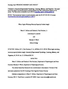
As pointed out almost 100 years ago (Soper, 1913) and repeatedly restated since (e.g., Fisher, 1915; Hotelling, 1953; Soper et al., 1917), e is negatively biased, that is, E(r) ⬍ , and the more so, the smaller n and the stronger . Graph A in Figure 1 (based on Soper et al., 1917) illustrates the magnitude of the negative bias of r for selected values of as a function of n. Consequently, NWT’s main argument—the positive bias of intuitive correlation estimates due to the limited WM capacity— clearly contradicts a basic statistical fact. It is worth noting that this argument does not stem from lack of awareness to this fact—which was mentioned in the theory’s original publication (Kareev, 1995b, p. 266, Footnotes 3 and 4) and illustrated by means of several numerical examples (based on David, 1954)— but rather from the evaluation of this fact as irrelevant to the discussion of the bias of r: “. . . the mean of the sampling distribution is of less consequence than the median or the mode, as the present discussion involves the values of rxy in samples most likely to be encountered” (Kareev, 1995b, p. 266, Footnote 3). Several courses of action are possible at this point: The first one is to dismiss NWT’s positive bias argument as plainly false and leave it at that. A second possibility is to attribute it to a different definition of bias, in terms other than a nonzero error mean. As previously mentioned, we found no such idiosyncratic definition, neither in the original formulation of the theory
Figure 1. (A) The bias of the sampling error e ⫽ r ⫺ , E(e), which is based on Soper et al.’s (1917) study, and (B) narrow window theory’s dichotomous sampling error ε, E(ε), which is based on David’s (1954) study, as a function of sample size (n) for selected positive values.
(Kareev, 1995a, 1995b) nor in latter publications (e.g., Kareev, 2000, 2003, 2005). A third possibility is that the error underlying the positive bias argument is not the sampling error e ⫽ r ⫺ , but some other (still unidentified) error. We suggest that this is, indeed, the case. Consequently, the valid interpretation of NWT’s argument in terms of positive bias (which is explicitly included in the very title of Kareev’s, 1995a, article as well as in latter publications) necessarily requires the specification of this error.
The Dichotomous Sampling Error (ε) of r and Its Bias We submit that the conceptualization of NWT’s amplification effect in terms of positive bias implicitly relies on a dichotomous function of the original sampling error e, ε ⫽ g共e兲:ε ⫽ ⫹ 0.50 if e ⬎ 0, and ε ⫽ ⫺ 0.50 if e ⬍ 0,
(2)
where epsilon (ε) distinguishes only between positive and negative sampling errors, assumed to be of equal magnitude and assigned the numerical values ⫹0.5 and ⫺0.5, respectively; that is, ε is a
CAHAN AND MOR
440
symmetrical directional sampling error.1 In line with the general definition, the bias of ε is defined as follows:
[in the sense of E(ε) ⬎ 0] and negatively biased [in the sense of E(e) ⬍ 0].
E共ε兲 ⫽ ⫺ 0.50 ⫻ P共e ⬍ 0兲 ⫹ 0.50 ⫻ P共e ⬎ 0兲 ⫽ 0.50 ⫻ 关P共e ⬎ 0兲 ⫺ P共e ⬍ 0兲兴.
Psychological Implications (3)
That is, ε is unbiased [E(ε) ⫽ 0] if and only if P(e ⬍ 0) ⫽ P(e ⬎ 0). An alternative definition of E(ε), which directly allows for its computation on the basis of the statistical tables of the sampling distribution of r (e.g., David, 1954), is given by Equation 4: E共ε兲 ⫽ 0.50 ⫺ Fr共兲,
(4)
where 1. Fr () ⫽ P(e ⬍ 0) is the cumulative relative frequency of in the distribution of r for sample size n and parameter [i.e., P(r ⱕ )], and 2. 0.50 is the value of Fr () when ε is unbiased [i.e., E(ε) ⫽ 0]. We submit that E(ε) is the (missing) implicit definition and measure of NWT’s amplification effect in terms of positive bias. According to Equation 4, E(ε) can be meaningfully interpreted as a proportion: the proportion of samples in which r ⬎ that is added to 0.50 because of small sample size. This interpretation is consistent with the probabilistic formulation of NWT’s positive bias effect (e.g., “more often than not”; Kareev, 2005, p. 280). Graph B in Figure 1, based on David’s (1954) tables according to Equation 4, gives the size of E(ε) as a function of n for selected positive values of . As illustrated by the diagram, E(ε) is positive (congruent with NWT’s assertion) albeit small. For example, for ⫽ 0.50 and 5 ⱕ n ⱕ 9, E(ε) ranges between 0.04 and 0.06. Furthermore, E(ε) is larger, the smaller the sample size (in accordance with NWT) and the stronger . It is interesting to note that, unlike E(e), E(ε) cannot be interpreted in terms of the magnitude relation between any central tendency measure of the sampling distribution of r and . The fact that, for small samples, both median(r) and mode(r) are more extreme than — offered as evidence for the amplification effect (Kareev, 1995b, p. 266)—is a result of E(ε) ⬎ 0 rather than its cause: Whereas [median (r) ⫺ ] ⬎ 0 indicates the existence of a positive bias of ε, it does not define or measure it.
e Versus ε To conclude, we suggest that the contradiction between NWT’s main statistical argument—the positive bias of the sample r for small samples—and the well-established statistical wisdom— according to which r is negatively biased, and the more so, the smaller the sample—is entirely attributable to the difference between the sampling errors on which they rely, e and ε, respectively. This contradiction is, in fact, a part-whole contradiction, one between the conclusion based on one component of the sampling error e—its sign, which underlies the definition of ε—and the conclusion based on the sampling error e itself (which consists of both sign and magnitude). The negative E(e) values for small samples reflect the higher average magnitude of the negative errors, which compensate (in fact, overcompensate) for their lower relative frequency. In contrast, E(ε) is positive because ε ignores the difference between positive and negative errors in terms of average magnitude. The sampling distribution of r for small samples can thus be validly described as being both positively biased
The Biasing Effect of WM Capacity Limitations on the Intuitive Assessment of Correlation: Positive or Negative? The main implication of the statistical analysis in the previous section is that the formulation and interpretation of NWT’s argument regarding the effect of limited WM capacity on the intuitive assessment of correlation in terms of positive bias is valid only for a dichotomous definition of error. Clearly, however, estimation error is not only a matter of sign. Magnitude matters. The psychological result of encountering a sample r that deviates ⫺0.30 from is likely to be different from that of encountering a sample r that deviates ⫺0.01 from . For example, the detection of a strong and useful regularity (e.g., ⫽ 0.50) will be strongly affected by a large negative sampling error (e.g., r ⫽ .20), but entirely unaffected by a small, same sign error (e.g., r ⫽ .49). In contrast, it can be safely assumed that the intuitive estimation of will not be affected by small sampling errors of opposite sign (e.g., r ⫽ .49 and r ⫽ .51). A valid psychological theory of sample-based intuitive correlation assessment should consider both the sign and the magnitude of the sampling error of r in small samples. Hence, the definition of bias in terms of e—rather than ε—is preferable not only on formal grounds, but also from substantive considerations. Outwardly, adoption of this definition leads to inversion of NWT’s main argument: Reliance on small samples due to capacity limitations results in negative, rather than positive, bias in correlation assessment. Nevertheless, we suggest that this conclusion, necessarily based on the average error, gives a misleading picture of the psychological effects of WM capacity limitations on the intuitive assessment of correlation. A conclusion based on error averaging [either E(ε) or E(e)] would have been psychologically meaningful had the intuitive assessment of correlation by each individual been based on the average of the withinindividual distribution of the sample r values between the same pair of variables, X and Y (e.g., height and weight) observed by him or her. In this case, the (contradictory) psychological implications of E(ε) ⬎ 0 and E(e) ⬍ 0 would have been universal: According to NWT, intuitive assessment of any by each and every individual is positively biased; according to our own analysis, bias is negative for each and every individual. However, despite the appeal of this possibility, the withinindividual distribution of sample rs is not involved, according to NWT, in the intuitive estimation of . Rather, the theory specifi1
The symmetrical numerical values that can be assigned to positive and negative errors are arbitrary (e.g., ⫹1 and ⫺1 or ⫹8 and ⫺8). Note, however, that the numerical value of E(ε) is specific to these arbitrary numbers and, therefore, meaningless. A metric-free measure of bias is obtained by standardizing ε by its range: ε , ε⬘ ⫽ ε max ⫺ ε min where εmax ⫺ εmin are the (symmetrical) arbitrary numerical values assigned to positive and negative errors, respectively. As a result of standardization, ε⬘ is independent of the arbitrary metric of ε: The same numerical ε⬘ values, ⫹0.5 and ⫺0.5, will obtain for any symmetrical εmax and εmin values.
COMMENTARY
cally assumes that each individual’s intuitive assessment of exclusively relies on the r computed in the first sample encountered and is not affected by subsequent samples (e.g., Kareev, 1995b, p. 264). Hence, the sampling distribution of r for small samples is not used by NWT to model the psychological process underlying the intuitive correlation estimation of each and every individual—which, as previously mentioned, is assumed to rely on a single r value— but only the across-individuals distribution of its results: the distribution of the rs between the same X and Y computed by all the individuals with a given WM capacity on the basis of the first random sample encountered by each of them. Hence, any bias argument [either E(ε) ⬎ 0 or E(e) ⬍ 0] can only apply, in the framework of NWT, to this distribution and necessarily involves averaging sampling errors across all the individuals with the same WM capacity in the population.
Average Versus Differential Effects Averaging errors across individuals is problematic from two perspectives. First, it has no empirical counterpart: No populationlevel estimate based on averaging rs across individuals is typically computed. Second, it ignores the between-individual variability of e, in terms of both sign and magnitude. Because, according to NWT, each individual estimate is based on a single sample, different individuals with the same WM capacity will encounter samples with different sampling errors: some positive and some negative, some large and some small. Consequently, the intuitive estimates of the same by different individuals will differ both in the direction and the magnitude of the estimation error they include: Some individuals will overestimate (by different amounts), whereas others will underestimate it (by different amounts). A realistic and valid psychological theory of intuitive correlation assessment should acknowledge these differential effects of reliance on small samples due to WM capacity limitations rather than focus on their population means. Furthermore, measurement of these effects requires a clear conceptual distinction between (a) the effect of the unavoidable reliance on samples in the intuitive assessment of correlations and (b) the net effect of the small size of these samples, due to capacity limitations, per se—that is, the net effect of WM capacity limitations. As a result of the former, intuitive estimates of (based on the first sample encountered) will necessarily include sampling error—albeit relatively small— even for large samples (e.g., 50, 100, or 400): ⬇50% of the individual estimates will be greater than (i.e., overestimates), and ⬇50% lower than (i.e., underesti-
441
mates; Fisher, 1973, p. 194). Reliance on small (rather than large) samples, due to WM capacity limitations (i.e., seeing the world through a narrow window; 关b兴 above), affects the intuitive assessment of correlation in two ways: 1. By increasing the proportion of individuals who overestimate , over and above the 50% base rate for large samples (and concomitantly decreasing the proportion of individuals who underestimate ), congruent with NWT’s main assertion. This net effect of WM capacity limitations is validly measured by E(ε)— Graph B in Figure 1. For most combinations of n and , the increase is modest (Mdn ⫽ 4%). 2. By increasing both the average amount of overestimation of [by the 0.50 ⫹ E(ε) individuals who encounter small samples in which r ⬎ ] and the average (absolute) amount of underestimation of [by the 0.50 ⫺ E(ε) individuals who encounter small samples in which r ⬍ ] – E(e|e ⬎ 0)n and E(e|e ⬍ 0)n, respectively—relative to their large sample (N) values, E(e|e ⬎ 0)N and E(e|e ⬍ 0)N, respectively. We refer to these effects as the amplification and attenuation effects of limited WM capacity, per se, ⌬(e⫹) and ⌬(e⫺), respectively: ⌬共e⫹ 兲 ⫽ E共e|e ⬎ 0兲 n ⫺ E共e|e ⬎ 0兲 N and ⌬共e⫺ 兲 ⫽ E共e|e ⬍ 0兲 n ⫺ E共e|e ⬍ 0兲 N.
(5)
Table 1 gives the numerical values of ⌬(e⫹) and ⌬(e⫺) as a function of n for selected values, assuming N ⫽ 400 (the largest value of N in David’s, 1954, tables). As indicated by Table 1: 1. Both the amplification and attenuation effects of limited WM capacity are considerable for all the combinations of and n: ⌬(e⫹) ranges between .10 and .55 (Mdn ⫽ .24), whereas ⌬(e⫺) ranges between ⫺.18 and ⫺.71 (Mdn ⫽ ⫺.33). 2. For any given , both effects are stronger, the smaller the WM capacity. 3. For any combination of and n, the (absolute) amount of attenuation exceeds the amount of amplification, and the more so, the smaller the n and the stronger the . Hence, contrary to Kareev’s (1995b, p. 268) unreserved claim that “. . . [limited capacity] acts as an amplifier, strengthening signals which may otherwise be too weak to be noticed,” our analysis points to a complex picture of the net effects of limited WM capacity (i.e., of the window’s “narrowness”) on the intuitive assessment of correlation, assuming exclusive reliance on the first (small) sample of the joint distribution of X and Y. Although limited capacity does indeed act as an amplifier for some individ-
Table 1 The Magnitude of the Attenuation and Amplification Effects of Limited Working Memory Capacity [⌬(e⫺) and ⌬(e⫹), respectively] as a Function of n for Selected Values Working memory capacity n⫽3
n⫽5
n⫽7
n⫽9
⌬(e⫺)
⌬(e⫹)
⌬(e⫺)
⌬(e⫹)
⌬(e⫺)
⌬(e⫹)
⌬(e⫺)
⌬(e⫹)
0.1 0.3 0.5 0.7
⫺.64 ⫺.69 ⫺.71 ⫺.65
.55 .44 .32 .19
⫺.40 ⫺.42 ⫺.40 ⫺.33
.36 .30 .22 .14
⫺.31 ⫺.32 ⫺.29 ⫺.23
.28 .24 .18 .12
⫺.26 ⫺.26 ⫺.24 ⫺.18
.24 .20 .16 .10
CAHAN AND MOR
442
uals, for other individuals it acts as a silencer, attenuating signals that may have otherwise been noticed. Furthermore, the (absolute) amount of attenuation always exceeds the amount of amplification. The average-based bias notion obscures this betweenindividuals variability in the effects of WM capacity limitations and may be misinterpreted as indicating the existence of a single, fixed, universal individual-level effect. Awareness of this variability is particularly critical for the evaluation of the adaptive value of the effects of limited WM capacity on the intuitive assessment of correlation and of the limited capacity itself.
The Adaptive Value of the Effects of Capacity Limitations on Intuitive Correlation Assessment The conclusions of our analysis are clearly inconsistent with Kareev’s (2000) unqualified positive evaluation of the adaptive value of the effects of limited WM capacity on intuitive correlation assessment as well as of the WM limitations themselves.2 The sizeable attenuation of r in the samples encountered by a substantial minority of individuals can hardly be defended as adaptive— that is, as protecting individuals “from missing strong correlations” (Kareev, 2000, p. 401). The overall evaluation of the adaptive value of limited capacity should not overlook this sizeable minority and concentrate exclusively on the small majority who encounter samples in which r is, indeed, amplified (i.e., r ⬎ ), as suggested in NWT’s original publication: “the present discussion involves the values of rXY in samples most likely to be encountered [italics added]” (Kareev, 1995b, p. 266, Footnote 3). Under the assumptions of NWT (particularly the exclusive reliance on the first sample encountered), small capacity is good for some people and bad for others, and, for each individual, it is sometimes good and sometimes bad.
2
The import of our analysis to this issue is entirely independent of the recent debate regarding it (Anderson et al., 2005; Juslin & Olsson, 2005; Kareev, 2005). This controversy was based on the acceptance of NWT’s main assertion regarding the existence of a sizeable positive bias in correlation assessment. Opinion differences only regarded the methods by which the effect of this positive bias on the detection of correlation should be evaluated and interpretation of their results.
References Anderson, R. B., Doherty, M. E., Berg, N. D., & Friedrich, J. C. (2005). Sample size and the detection of correlation—A signal detection ac-
count: Comment on Kareev (2000) and Juslin and Olsson (2005). Psychological Review, 112, 268 –279. Cleary, T. A. (1968). Test bias: Prediction of grades of Negro and White students in integrated colleges. Journal of Educational Measurement, 5, 115–124. David, F. N. (1954). Tables of the correlation coefficient. Cambridge, England: Cambridge University Press. Feldt, L. S., & Breman, R. C. (1989). Reliability. In R. L. Linn (Ed.), Educational measurement (3rd ed., pp. 105–146). New York: American Council on Education. Fisher, R. A. (1915). Frequency distribution of the values of the correlation coefficient in samples from an indefinitely large population. Biometrika, 10, 507–521. Fisher, R. A. (1973). Statistical methods for research workers. Oxford, England: Oxford University Press. Hotelling, H. (1953). New light on the correlation coefficient and its transforms. Journal of the Royal Statistical Society, Series B, 15, 193– 232. Juslin, P., & Olsson, H. (2005). Capacity limitations and the detection of correlations: Comment on Kareev (2000). Psychological Review, 112, 256 –267. Kareev, Y. (1995a). Positive bias in the perception of covariation. Psychological Review, 102, 490 –502. Kareev, Y. (1995b). Through a narrow window: Working memory capacity and the detection of covariation. Cognition, 56, 263–269. Kareev, Y. (2000). Seven (indeed, plus or minus two) and the detection of correlations. Psychological Review, 107, 397– 403. Kareev, Y. (2003). On the perception of consistency. Psychology of Learning and Motivation, 44, 261–285. Kareev, Y. (2005). And yet the small-sample effect does hold: Reply to Juslin and Olsson (2005) and Anderson, Doherty, Berg, and Friedrich (2005). Psychological Review, 112, 280 –285. Kareev, Y., Lieberman, I., & Lev, M. (1997). Through a narrow window: Sample size and the perception of correlation. Journal of Experimental Psychology: General, 126, 278 –287. Lord, F. M., & Novick, M. R. (1968). Statistical theories of mental test scores. Reading, MA: Addison-Wesley. Mood, A. M., Graybill, F. A., & Boes, D. C. (1987). Introduction to the theory of statistics. Singapore: McGraw-Hill. Soper, H. E. (1913). On the probable error of the correlation coefficient to a second approximation. Biometrika, 9, 91–115. Soper, H. E., Young, A. W., Cave, B. M., Lee, A., & Pearson, K. (1917). On the distribution of the correlation coefficient: Appendix II to the papers of “student” and R. A. Fisher. Biometrika, 11, 328 – 413. Stanley, J. C. (1971). Reliability. In R. L. Thorndike (Ed.), Educational measurement (2nd ed., pp. 356 – 442). Washington, DC: American Council on Education.
Received January 18, 2006 Revision received August 16, 2006 Accepted August 29, 2006 䡲