The Effects of Fault Counting Methods on Fault Model Quality Allen P. Nikora Jet Propulsion Laboratory, California Institute of Technology Pasadena, CA 9 1109-8099
[email protected]
Abstract Over the past several years, we have been developing software fault predictors based on a system’s measured structural evolution. We have previously shown there is a signiJcant linear relationship between code chum, a set of synthesized metrics, and the rate at which faults are inserted into the system in terms of number of faults per unit change in code chum. A limiting jbctor in this and other investigations of a similar nature has been the absence of a quantitative, consistent, and repeatable definition of what constitutes a fault. The rulesfor fault definition were not sujiciently rigorous to provide unambiguous, repeatablefault counts. Within theframework of a space mission software development eflort at the Jet Propulsion Laboratoiy (JPL) we have developed a standard for the precise enumeration offaults. This new standard permits so@warefaults to be measured directlyJLom configuration control documents. Our results indicate that reasonable predictors of the number of faults inserted into a software system can be developed JLom measures of the system’s structural evolution. We compared the new method of counting faults with two misting techniques to determine whether the fault counting technique has an effect on the quality of the fault models constructed fiom those counts. The newfault definitionprovides higher qualityfault models than those obtained using the other de3nitions of fault.
KEYWORDS: defect content estimation techniques, fault prediction, software measurement, software modeling.
John C. Munson Chief Science Officer Cylant, Inc. Lexington, MA 02421
[email protected]
1. Introduction Over the past several years, we have been investigating relationships between measurements of a software system’s structural evolution and the rate at which faults are inserted into that system [Muns98, Niko98, NikO031. Measuring the structural evolution of a so% ware system has proven to be a well-defined task that can easily be automated. Unfortunately, it has not been as easy to measure the number of faults inserted into the system - there has been no quantitativedefinition of just precisely what a software fault is. In the face of this difficulty it is hard to develop meaningful associative models between faults and code attributes. Since code attributes are collected at the module level, we strive tu collect information about faults at the same granularity. We have recently developed a quantitative definition for software faults that allows automated identification and counting of those faults at the module level [MunsO2]. Using this definition, we have identified strong relationships between measured structural change to a software system and the number of faults inserted into that system [Nikd3]. The results obtained in collaboration with the Mission Data System (MDS), a space mission software technology development effort at JPL [Dvo99] indicate that our technique of counting faults can be used to develop fault models with good predictive power. However, there are other ways of counting software faults besides the technique we proposed. In this paper, we describe three other fault-counting techniques and compare the models resulting from the application of two of those methods to the models obtained from the application of our proposed definition.
2. Related Work Over the past several years, researchers have developed a number of fault predictors based on measurable characteristics of a software system. Examples include the classification methods proposed by Khoshgoftaar and Allen WosOla] and by Gokhale and Lyu [Gokh97], Schneidewind’s work on Boolean Discriminant Functions [Schn97], Khoshgoftaar’s application of zero-inflated Poisson regression to predicting software fault content [KhosOl], and Schneidewind’s investigation of logistic regression as a discriminator of software quality [SchnOl]. Each of these has provided useful insights into the problem of identifjmg fault-prone software components prior to test. However, these studies used different &finitions at varying levels of precision of what constitutes a fault. For example, the definition of the ‘%hult” response variable reported in WosOla] is ‘’the number of faults discovered in a source file”. The definition used in [Schn97] and [SchnOl] is the number of Discrepancy Reports (DRs) written against modules, where the DRs record observed deviations from requirements. This definition is repeatable for the system under study, and is related to a system’s quality. However, it refers to the number of failures rather than the number of faults. Neither do current standards seem to provide quantitative definitions for faults. The following definition of what constitutes a fault is typical of that provided by current standards: “A manifestation of an error in software. A fault, if encountered, may cause a failure” [IEEE88, IEEE831. This establishes a fault as a structural defect in a software system that may cause the system to fail, but does not help in determining how individual faults may be identified or measured. During a small study on a JPL flight system several years ago [Niko98], we recognized the importance of developing a standard, quantitative definition for faults. In an attempt to define an unambiguous set of rules for identifying and counting faults, we developed an empirical taxonomy based on the types of editing changes we observed in response to reported failures in the system [Niko97]. We found strong indications that a system’s measured structural evolution could predict the fault insertion rate. However, the d e f ~ tion of faults that was used was not quantitative. Although the rules provided a way of classifying the faults, and attempted to address faults at the module level, they were not sufficient to enable repeatable and consistent fault counts by different observers.
Four years ago, we started a collaborative effort with the MDS to address this limitation of the earlier study. Our main concern was developing a quantitative definition of faults, so that we could automate what had been a time-consuming manual activity in the earlier study, the identification and counting of repaired faults at the module level. Our hope was that this would provide us with unambiguous, consistent, and repeatable fault counts. For our study, the structural evolution of the MDS was measured over a period from October 20, 2000, through April 26, 2002. The system contains over 15000 distinct modules; over the time interval analyzed studied, there were over 1500 builds of the MDS. The total number of distinct versions of all modules was greater than 65,000. Over 1400 problem reports were included in the analysis; these problem reports provided the information from which the number of repaired faults was computed.
3. Problem Statement The overall objective of our work is to develop practical methods of predicting software fault content based on measurable characteristics that can be used by software development efforts to help them better manage the quality of their systems. We searched relationships between the rate at which faults are inserted into source code and the measured structural evolution of the source code. Such a relationship would allow us to estimate the system’s fault content at any time during its development. This process, however, is predicated on our ability to define precisely software faults and to measure them with a high degree of precision. The driving force behind modeling the relationship between software faults and software attributes such as size is that we can measure software attributes directly, It is possible to develop stringent standards for measuring source code. Measuring software faults is quite another matter. Fault measures can either be relatively fine grained or coarse grained. We will identify three distinct methods of measuring faults and then model the relationship of certain software attributes to these different fault measurement strategies. Although other types of software artifacts could have been analyzed, source code has two advantages: 0 Measuring its structural attributes is easily automated. Since the source code is controlled by a configuration management system, different versions of the system can be easily and unambiguously identified. In particular, a baseline against which
all other versions are to be measured can be easily established. The objective of this paper, then, is to model the relationship of specific software attributes with the fault predictors created using our recently developed fault counting technique and compare this model with fault predictors developed using other proposed methods of counting faults.
complexity, as is shown by the relatively high values (>0.85) of the Nodes and Edges metrics in this table. Domain 2 is most closely associated with the variety of data processed by a module and the operations performed; Domain 3 is associated with the number of distinct paths through the module. The raw metrics most closely associated with underlying orthogonal domain are shown in boldface t w e in Table 2. I I
4. Structural Metrics Used in this Study The software attribute measurement data for this study were obtained from the Darwin system [CylaO3] that was used to measure and manage metric data on the target software system. These data were obtained by checking out each build of the system from the confguration control system and then applying the measurement tools incorporated in the Darwin Network Appliance. The Darwin system collected measurement data across the multiple builds of the target systems.
4.1.
N,
I
frotaloperatorcount
Software Attribute Measures
The software attributes that were measured for this study are shown in Table 1. These measures were obtained for both the C and the C+c code modules in the MDS system. The precise definition of each of these measures and the standard used to measure them can be found in [MunsOZa]. All measurements were taken at the module level. For C program elements, a module is a function. For C U a module is a function or an object.
4.2.
I
is
Derived Metrics
Our previous work has shown that the metrics shown in Table 1 are highly correlated [Muns90, HdlOO]. Using principal components analysis (PCA) [Di184], we identified the distinct orthogonal sources of variation and mapped these twelve raw metrics onto a set of uncorrelated metrics that represent essentially the same information. We stopped extracting components when the eigenvalues associated with a component assumed values less than 1. The PCA results are shown in Table 2. The eigenvalues are shown as the last row of Table 2 - the sum of all of the eigenvalues for the 12 original metrics is 12.0. The three domains together account for approximately 85% of the total variation observed in the original 12 metrics. We found three distinct sources of variation in the twelve original raw metrics that we have labeled as Domain 1, 2, and 3 in Table 2. Domain 1 is most closely associated with the control flow attributes relating to the module's control flow graph structure
It is necessary to standardize all original or raw metrics so that they are on the same relative scale. For the thmodule m;on thej" build of the system there will be a data vector X; =.x:,,x;z,...,x,:z > of 12 raw metrics for
that module. We standardizeeach of the k raw metrics by subtracting the mean zi of the metric k over all modules in thefh build and dividing by its standard deviation a: such that 2: = (xi -Z;)/a; represents the standardized value of the Ph raw metric for the th module on thefh build. A by-product of the original PCA of the 12 metric primitives is a transformation matrix, T that maps the z-scores of the raw metrics into the reduced space represented by the three principal compondnts. Let Z represent the matrix of z-scores shown in Table 2 above for the original problem. We obtain new domain metrics, D, using the transformation matrix T as follows: D = ZT where Z is an n by 12 matrix of zscores, T is a 12 x 3 matrix of transformation coefficients, and D is a n x 3 matrix of domain scores where n is the number of modules being measured in a particular build. The matrix, T,for this solution given in columns 2 through 4 of Table 3. The means and standard deviations used to compute the z-scores are also shown in columns 5 and 6 of Table 3. For each module, there are now three new metrics, each representing one the three orthogonal principal components. These domain scores are uncorrelated, thereby eliminating the problem of multicollinearity fkom the linear regression models that we wish to develop.
5. Measuring Software Faults One of the major problems in the analysis of software faults and their relationship to measurable software attributes is the lack of a standard way of counting faults. Because of this, previous attempts to develop models of software quality are of questionable value. We define below three different approaches to fault measurement fkom a very low level token based measure to a high-level failure report level measure.
5.1.
Token-Based Fault Counts
One of the most important considerations in the measurement of software faults is the ability to scale the fault. Sometimes a simple operator is at fault; the developer used a "+" instead of a "-". Other times two or three statements must be modified, added, or deleted to remedy a single fault. Further, some program changes to fix faults are substantially larger than are others. We would like our fault count to reflect that fact. The actual changes made to a code module are tracked in configuration control systems such as RCS or CVS [Cede931 as code deltas. We must learn to classifl the code deltas that we make as to the origin
of the fix. In other words, each repair action for each module should reflect a specific code fault fix, a design problem, or a specificationproblem. If we change any code module and fail to record each fault as we repair it, we lose the ability to resolve faults for measurement purposes. The important consideration with any fault measurement strategy is that there must be some indication as to the amount of code that has changed in resolving a problem in the code. We have regularly witnessed changes to tens or even hundreds of lines of code recorded as a single "bug" or fault. The number of tokens that have changed to ameliorate the original problem constitutes a measurable index of the degree of the change. To simplify and disambiguate further discussion, consider the following definitions. Definirion: A fault is an invalid token or bag of tokens in the source code that may cause a failure when the compiled code implementing the tokens is executed. Deflnirion: A failure is the departure of a program from its specified hctionalities. Definition: A defect is an apparent anomaly in the program source code. By taking as the fault count the number of tokens that have changed, we take into account the sue and extent of the fault. Each line of text in each version of the program can be seen as a bag of tokens. When a developer changes a line of code in response to the detection of a fault, the tokens on that line will change. New tokens may be added, invalid tokens may be removed, or the sequence of tokens may be changed. Enumeration of faults under this definition is unambiguous and consistent, and can be automated. This definition of fault eliminates the errors introduced by existing ad hoc fault reporting schemes [MunsOZ, Muns02al. The following example shows this fault measurement process. Consider the following line of C code. (1) a = b + c ; There are five tokens on this line of code. They are B1 = {
, , , , ,, , < e ) . The bag difference is B1 B2 = {, .e-> }. The cardinality of B1 and B2 is the same. There are two tokens in the difference. Clearly, one token has changed
-
fi-om one version of the module to another, indicating one fault. Now suppose that the problem introduced by the code in statement (2) is that the order of the operations is incorrect. It should read: (3) a = c - b ; The bag for this neiw lime of code will be B3 = {, , ,
templateint ILDc Mds::Fw:Car::Lcki::NullType >::addDspendencyTcConConnedor(cDnatMds::Fw:lnit::lnitFunctoleasee P unnector ‘I) > ( > return 0; > } > > template cdass Ur > int lL~U,::addDependencyToConnector(const Mds::Fw::lnit::lnitFunctw8as& connector) >
>
( return InterfaceListbpendencycU>::addbpendency‘ToConnector(carne;
>
I
>
22c34 void l n t e r f a c e L i s t D e p e n d e ~ C T ~ P : : ~ d ~ p e ~ ~ T ~ n e c t o r ( ~ ~
c
-Mds::Fw:lnit::lniffundorBase& connector) > int I n t e r f a c e l i s t D e p e n d e n ~ c 1 ~ s ~ : : a d d D e p e n Mds::F~:lne:lnitFunctorease(lconnector)
2-38 return
>
29,31c42,43 C
connedor);
c C I
connector) +
>
35,39d46 template vud I L D s U > : : a d d D e p e n d e n c n ~ ~ c o n s t Mdr:Fw:lnit::lnitFunctorBase& connector) c
2 -
{ lnterfecelisIDependenoyU>::addDependency; 1
Figure 1 - Differential Comparison of Faulty, Repaired Module
5.4.
Number of Failure Reports
A popular method of approximating the number of faults is to simply count the number of failure reports. At the system level, this technique can work quite well - in fact, we have shown that there is a high correlation (> 0.9) between counts of the number of observed failures and measurements of the amount of structural
change experienced by the system as a whole [Niko03a]. However, we chose not to include failure counts in this study because of the problem o f scaling them to the level of individual modules. An individual failure may result in changes to more than one module, as shown in Figure 2. To use failure counts at a module level, it would be necessary to count a failure report multiple times; specifically, for each module repaired in response to that failure report, the number o f
failures for that module would need to be increased by 1. This assumes that if one of the modules were not changed, the failure would occur. We were not cornfortable making this assumption without a detailed analysis of the repair actions, which was beyond the scope of this study.
changed module. We will refer to this reconfiguration as a build. For the effect of any change to be felt it must physically be incorporated in a build. The first step in the measuring the evolutionary development of a software system is to establish a baseline reference point in the build process. W h e n a number of successive system builds are to be measured, we choose one of the systems as a baseline system. All others will be measured in relation to the chosen system. We must standardize the metric scores in a way that will not erase the effect of trends in the data. For example, let us assume that we were taking measurements on LUC and that the system we were measuring grew in this measure over successive builds. We will standardize the raw metrics using a baseline system such that the standardized metric vector for the i"' module m,' on the j" build would be
.:
where : E is a vector containing the means o f the raw metrics for the baseline system and is a vector of standard deviations o f these raw metrics. Thus, for each system,we may build an m x k data matrix, Z', that contains the standardized metric values relative to the baseline system on build B. Table 3 - The Measurement Baseline
= a-m
-
.
>
=
e
Y
-- - -.-
91LE m s r : 1 1 1 Y ; w 1 w W -m .-'lMlY10011*01 w
-.
I-
-
J
Y inrrn
P
1-
I
d
r y
M "d
u l ~ w m mm l m r m
.L
Figure 2 -Failure Report Identifying Changes
6. The Measurement Baseline A complete software system generally consists of a large number of program modules. Each of these modules is a potential candidate for modification as the system evolves during development and maintenance. As each program module is changed, the total system must be reconfigured to incorporate the
W h e n we have identified a target build, B, to be the baseline build we will then compute the three constituent elements o f the baseline. These elements are the transformation matrix for the baseline build, the vector
T"
o f metrics means for the baseline build i:, and a vecB
tor C , of standard deviations for this build. For the
purposes of this study, the July 1,2001 build was chosen as the baseline build. Table 3 presents the baseline we used to compute the derived metrics.
7. Measuring Change Activity In order to describe the complexity of a system at each build, it is necessary to know which version of each module was in the program at any point in time. Consider a software system composed of n modules as follows: m l ~ m 2 ~ m 3 * * " ~ m n . Not all of the builds will contain precisely the same modules; there will be different versions of some of the modules in successive system builds. Details are given in [MunsO2a]. We represent the build configuration in a nomenclature that permits us to describe the measurement process more precisely by recording module version numbers as vector elements in the following manner: v' =cVf,v;,vJI,..-V; > . This build index vector will allow us to preserve the precise structure of each for posterity. Thus, V,n in the vectorv" would represent the version number of the i" module that went to'n build of the system. The cardinality of the set of elements in the vector V" is determined by the number of program modules that have been created up to and including the nthbuild. In this case the cardinality of the complete set of modules is represented by the index value m. This is also the number of modules in the set of all modules that have ever entered any build. When evaluating the precise nature of any changes that occur to the system between any two builds i, and j , we are interested in three sets of modules. The first set, M:', is the set of modules present in both builds of the system. These modules may have changed since the earlier version but were not removed. The second set, M :' ,is the set of modules that were in the early build, i, and were removed prior to the later build, j . The final set, MI;J ,is the set of modules that have been added to the system since the earlier build. Details of the measurement process are given in wunsO2a]. With a suitable baseline in place, software evolution across a full spectrum of software metrics can be measured. We do this first by comparing average metric values for the different builds. Secondly, we can measure the changes in the domain metrics, or we can measure the total ainount of change to the system across all of the builds to date. The change in domain score in a single module between two builds may be measured as the absolute
value of the difference in domain scores on these two builds. We will call this code churn measure domain churn. In the case of code churn, what is important is the absolute measure of the nature that code has been modified - faults can be inserted by removing code as well as by adding code. Let d? represent the zh domain score of the dh module on build j baselined by build B. The new measure of domain churn, ,for module ma is simply That is, the domain churn may be established by computing the baselined domain scores for any two builds and then find the absolute difference between these values. This represents the relative amount of change activity that there has been on each of the three domains between any two builds. Now we wish to characterize, or measure, the complete change to the system over all of the builds f7om build 0 to build L. Many modules, however, may have come and gone over the course of the evolution of the system. We are only interested in the history of the survivors; those modules that are now in the final build L. The total domain change activity of the system for module m, on domain i is the sum of the domain churn for this module f7om the point of its first introduction to the final build L is given by *;k
=Id?-
d;kl.
L-1
x: = Cx;J+l. J*
The value of the domain churn Xi for each module is, of course, dependent on the referent baseline build B. Note that if module m, were not present on buildsj and j + l , then X:J+I = 0 . Also, if module m, had been introduced on buildj+l then x;~+l = I d y l .
8. Relationships Between the Different Software Fault Counts and Change Activity In this investigation, we computed domain scores all of the available builds of the MDS system. These domain scores were baselined relative to the July 7,2001 build of the system, a build more or less intermediate in the sequence of builds. Since the initial build is generally quite incomplete, it is a good idea to change the baseline as development progresses. The next step in this investigation was to compute the fault count for each program module, using information available f7om the Internal Anomaly Report (IAR) system. All changes to the software were tracked under the CCC Harvest version control system (now
incorporated into Computer Associates’ CM systems see [CAO2]). Each change to a program module was made either as an enhancement or in response to a particular IAR. If a module code delta was attributed ”to an IAR, then the faults attributed to that change were calculated using the three different techniques described in Sections 5.1,5.2, and 5.3. After establishing each type of fault count for each incremental module version, the fault counts were accumulated so that by the f m l build a cumulative fault count of that type was available for each module in the final build. The fault counts for modules not in the final build vanished with the module domain churn values when the modules disappeared h m the evolving builds. To investigate the relationship between the fault content of models and the domain metrics, we eliminated those modules whose fault count was zero. There are two very good reasons for eliminating these modules. First, a zero fault count for a module on the last build does not imply that there are no faults in this module. It could very well mean that the faults have yet to be discovered. Second, approximately 90% of the modules in the final build have zero fault values. They would clearly dominate any regression model that was developed using them. With the data fiom the remaining modules, we developed three multiple linear regression models, one for each type of fault count, with the cumulative fault count as the dependent variable and the domain churn values as independent variables. The regression ANOVAs for these analyses are shown in Table 4. For each type of fault count, there is a distinct association with module change activity as measured by each of the three distinct fault counts and the module domain churn metrics as a measure of code evolution.
The regression models corresponding to the different types of fault counts are shown in Table 5 . For the models corresponding to the fault counts produced by computing token differences or counting the number of “sed” commands, Domain 1 is significant. For the model produced with token differences, Domain 1 dominates, and Domains 2 and 3 do not contribute to our understanding of the fault introduction process. The regression coefficients for these terms are not significant (p>0.05). For the model produced with fault counts produced by counting “sed” commands, Domain 2 contributes to our understanding of the fault insertion mechanism, and indeed dominates the model. Finally, for the model produced with counts of the number of modules changed, Domains 2 and 3 are the important factors in this model. Domain 1 plays no significant role. The three regression models, however, are not at all similar when we examine their predictive quality as measured by the R2statistic. This statistic is the ratio of sums of squares due to regression to the sums of squares total. Finally, we want to know something about the relative quality of the regression model that we have developed. These data are shown in Table 6. We can see from this table that for the model obtained fiom fault counts based on token differences (Model l), the adjusted R2 is approximately 0.61. This means, roughly, that we can account for approximately 60% of the variation in the cumulative fault count with the cumulative domain churn for Domain 1. This is a very respectable value for the limited metric set that the Darwin tool currently uses. For Models 2 and 3, we see that we can only account for a considerably smaller (less than 20%) percentage of the variation in the cumulative fault count with the cumulative churn in Domains
1, 2, and 3. Clearly, Models 2 and 3 are not usehl predictors. Table 6 -Model Quality I Model 1 R I Ad- IStdErrorI
Within the framework of this investigation, it is evident that we can develop higher quality fault predictors using fault counts based on token differences than either of the other types of fault counts described in Section 5. In the token-based module change model shown in Table 5 , the dominant factor was measurable changes
in the control structure of a module. Among the set of 12 metrics used in this investigation, those metrics most closely associated with the observed variation in software faults were the control metrics shown in the first principal component (Domain 1) of Table 2.
9. Discussion and Future Work We have seen that the method by which faults are counted can have a significant effect on the fault predictors developed using those counts. Of the predictors developed as part of this study, the one having the highest quality was based on the token-based fault counting technique we developed in m earlier phase of this work. We have also seen that by using an appropriate fault counting technique, predictors with a relatively high degree of accuracy can be developed. For the predictor developed from fault counts based on token differences, about 60% of the variation in the cumulative fault count was explained by our set of measurements, although the number of measurements used in the study was rather limited. This is a sufficiently large value for development efforts to start using these measurements as a management tool. We have, then, developed a functional definition of s o h a r e faults that can be applied to source code revision management systems for the automatic measurement of s o h a r e faults. Further, this definition allows faults to be unambiguously measured at the level of individual modules. Since faults are measured at the same level at which structural measurements are taken, meaningful models relating the number of faults inserted into a s o h a r e module to the amount of structural change made to that module can be developed. This measurement process makes it much more practi-
cal to analyze large software systems such as those developed to support NASA flight missions. Future work will involve investigation of these relationships for additional software development efforts at JPL and other NASA centers. Although fault counts based on token differences resulted in the highest quality fault predictor for this study, there is insufficient data at this point to generalize this conclusion. Detailed analysis of additional software development efforts is required before more general conclusions can be reached. We have started collaborative efforts with additional projects at P L to perform this investigation; we have also started working with the Software Assurance Technology Center at the Goddard Space Flight Center to investigate development efforts at other NASA centers. There may be uncontrolled sources of noise, which we intend to address in future work. For example, developers might be making enhancements to the system at the same time they are responding to a reported failure. In this case, the enhancements would be counted as repairs made in response to the failure. Addressing this issue will involve selecting an appropriate subset of the reported failures and interviewing developers about the changes made in response to those failures. We will be careful to select representative failures from all system components to control for the noise inserted by each development team. We will also select reported failures from different times during the development effort, to determine whether the number of enhancements reported as fault repair changes over time.
Acknowledgments The work described in this paper was carried out at the Jet Propulsion Laboratory, California Institute of Technology. This work was sponsored by the National Aeronautics and Space Administration’s Office of Safety and Mission Assurance (OSMA) S o h a r e Assurance Research Program (SARP),which is administered by NASA’s IV&V Facility. The authors also wish to thank the MDS project for the cooperation that made this study possible. Finally, we thank our colleagues who reviewed earlier versions of this paper and made many helpful suggestions.
References [CAO2]
Computer Associates, “AIlFusion Harvest Change Manager Features, Descriptions t Benefits”, Feb. 11,2002, available at: _htt~://www3.~acom/FileslFactSheet/af harvest an f d b d f
[Cede931 Per Cederqvist, “Version Management with CVS for C V S 1.1 l.lpl”, available at: httv://ww w.cvshome.orddocs/manual/. [Chid941 S. Chidamber, C. Kernerer, “A Metrics Suite for Object Oriented Design”, IEEE Transactions on Software Engineering, vol. 20, no. 6, June, 1994, pp. 476-493. [CylaO3] “The Darwin Software Engineering Measurement Appliance“, Cylant, available at: httu:l/mv.cvlan t.com/ [Di184] W. Dillon, M. Goldstein, Multivariate Analvsis: Methods and ADdications, Wiley-Interscience, 1984, ISBN 0471083178 [DvoW] D. Dvorak, R Rasmussen, G. Reeves, A. Sacks, “Software Architecture Themes In PL’s Mission Data System”, AIAA Space Technology Conference and Exposition, Sep. 28-30, 1999, Albuquerque, NM. [Goa971 S. S. Gokhale, M. R Lyu, “Regression Tree Modeling for the Prediction of Software Quality”, proceedings of the Third ISSAT International Conference on Reliability and Quality in Design, pp 31-36, Anaheim, CA, March 12-14, 1997 [Ha11001 G. A. Hall, J. C. Munson, “Software evolution: code delta and code chum”, Journal of Systems and Software 54 (2) (2000) pp. 111-118 [IEEE83] “IEEE Standard Glossary of Software Engineering Terminology”, IEEE Std 729-1983, Institute of Electrical and Electronics Engineers, 1983. [IEEE88] ‘WEE Standard Dictionary of Measures to Produce Reliable Software”, IEEE Ski 982.11988, Institute of Electrical and Electronics En~neers.1989. [KhosOl] T. -khoshgoftaar, “An Application of ZeroInflated Poisson Regression for Software Fault Prediction”, proceedings of the 12th International Symposium on Software Reliability Engineering, pp 66-73, Hong Kong, Nov, 2001. [KhosOla] T. M. Khoshgoftaar, E. B. Allen, “Modeling Software Quality with Classification Trees”,in H. Pham (ed), Recent Advances in Reliability and Oualitv Endneering, Ch. 15, pp 247-270, World Scientific Publishing, Singapore, 2001. [MUns90] J. C. Munson and T. M. Khoshgoftaar, “Regression Modeling of Software Quality,” Information and Software Technology, Vol. 32 No. 2 . 14. March 1990, p ~ 105-1
[Muns98] J. Munson and A. Nikora, “Estimating Rates Of Fault Insertion And Test Effectiveness In Software Systems” Proceedings of the Fourth ISSAT International Conference on Reliability and Quality in Design, August 12-14, 1998 pp. 263-269. [MunsOZ] J. Munson, A. Nikora, “Toward a Quantifiable Definition of Software Faults”, Proceedings of the 13th IEEE International Symposium on Software Reliability Engineering, IEEE Press. [MunsO2a] J. Munson, Software Encrineerine Measurement, CRC Press, 2002, ISBN 08493 15034. [Niko97] A. Nikora, J. Munson, “Finding Fault with Faults: A Case Study”, with J. Munson, proceedings of the Annual Oregon Workshop on Software Metrics, Coeur d’Alene, ID, May 1113, 1997. [Niko98] A. P. Nikora, J. C. Munson, “Determining Fault Insertion Rates For Evolving Software System’’, proceedings of the 1998 IEEE International Symposium of Software Reliability Engineering, Paderbom, Germany, November 1998, IEEE Press. [NikoOl] A. Nikora, J. Munson, “A Practical Software Fault Measurement and Estimation Framework’’, Industrial Presentations proceedings of the 12th International Symposium on Software Reliability Engineering, Hong Kong, Nov 2730,2001. mikd)3] A. Nikora, J. Munson, “Developing Fault Predictors for Evolving Software Systems”, proceedings of the 9th International Software Metncs Symposium, Sep 3-5, Sydney, Australia [Nikd33a] A. Nikora, J. Munson, “Understanding the Nature of Software Evolution”, proceedings of the International Conference on Software Maintenance, Sep 22-26, Amsterdam, The Netherlands. [Schn97] N. F. Schneidewind, “Software Metrics Model for Integrating Quality Control and Prediction”, proceedings of the 8th International Symposium on Software Reliability Engineering, pp 402415, Albuquerque, NM,Nov, 1997. [SchnOl] N. F. Schneidewind, “Investigation of Logistic Regression as a Discriminant of Software Quality“, proceedings of the 7th International Software Metrics Symposium, pp 328-337, London, April, 2001.