THE JOURNAL OF CHEMICAL PHYSICS 122, 104907 共2005兲
The effects of Lowe–Andersen temperature controlling method on the polymer properties in mesoscopic simulations Li-Jun Chen, Zhong-Yuan Lu,a兲 Hu-Jun Qian, Ze-Sheng Li,b兲 and Chia-Chung Sun State Key Laboratory of Theoretical and Computational Chemistry, Institute of Theoretical Chemistry, Jilin University, Changchun 130023, China
共Received 10 November 2004; accepted 27 December 2004; published online 14 March 2005兲 Lowe–Andersen 共LA兲 temperature controlling method 关C. P. Lowe, Europhys. Lett. 47, 145 共1999兲兴 is applied in a series of mesoscopic polymer simulations to test its validity and efficiency. The method is an alternative for dissipative particle dynamics simulation 共DPD兲 technique which is also Galilean invariant. It shows excellent temperature control and gives correct radial distribution function as that from DPD simulation. The efficiency of LA method is compared with other typical DPD integration schemes and is proved to be moderately efficient. Moreover, we apply this approach to diblock copolymer microphase separation simulations. With LA method, we are able to reproduce all the results from the conventional DPD simulations. The calculated structure factors of the microphases are consistent with the experiments. We also study the microphase evolution dynamics with increasing N and find that the bath collision frequency ⌫ does not affect the order of appearing phases. Although the thermostat does not affect the surface tension, the order-disorder transition 共ODT兲 is somewhat sensitive to the values of ⌫, i.e., the ODT is nonmonotonic with increasing ⌫. The dynamic scaling law is also tested, showing that the relation obeys the Rouse theory with various ⌫. © 2005 American Institute of Physics. 关DOI: 10.1063/1.1860351兴 I. INTRODUCTION
Polymers are widely used in industry and everyday life due to the chemical variability of the constituent molecules and their multiple mechanical properties. Computer simulation methods are ideally suited to help us understand the structures that lead to those properties and to enhance our ability of material design. For example, microscopically molecular dynamics 共MD兲 simulation techniques are always adopted to study the local chain relaxation dynamics in short time regime, and the finite element methods 共FEM兲 are widely applied in polymer processing simulations. However, polymers have a unique feature, that is, the existence of a relevant length scale in between the atomistic scale and the macroscopic scale. Such a length scale is beyond the reach of the traditional MD and FEM. Thus various simulation methods have been developed to study the mesoscopic structures, e.g., the time-dependent Ginsburg–Landau theory 共TDGL兲, the dynamic density functional theory 共DDFT兲,1,2 the lattice Boltzmann equation 共LB兲,3,4 the mean-field theory 共MF兲,5 and the dissipative particle dynamics 共DPD兲.6–9 The TDGL and DDFT have been successfully used, for example, to simulate spinodal decomposition in binary and ternary polymer blends and block copolymers, both in bulk and near surfaces.10 Recently LB method is coupled with MD to simulate polymer solution dynamics. With a beadspring lattice model, the polymer is treated on a coarsegrained molecular level, and the solvent molecules are treated on the level of a discretized Boltzmann equation.11 The MF and DPD represented by coarse-grained molecular a兲
Electronic mail:
[email protected] Electronic mail:
[email protected]
b兲
0021-9606/2005/122共10兲/104907/8/$22.50
models are utilized to study the morphology of inhomogeneous materials via Flory–Huggins parameters between components.10 DPD is a mesoscale simulation technique developed to model Newtonian and non-Newtonian fluids and correctly describes the hydrodynamic interactions.12–15 In a typical DPD simulation, the fluid is modeled as a collection of soft particles which individually represent many molecules. Interparticle interactions are characterized by pairwise conservative, dissipative, and random forces acting on a particle i by a particle j. The dissipative forces in DPD depend on the velocities, which in turn are governed by the dissipative forces. Therefore care must be taken when integrating the equations of motion in DPD framework. Groot and Warren 共GW兲 suggested a modified velocity-Verlet algorithm 共VV兲, in which an adjustable parameter was used to partially taking into account the force-velocity interdependence.9 DPD-VV16,17 is also a modified velocity-Verlet algorithm, which updates the dissipative forces for a second time at the end of each integration step. Shardlow’s splitting method is another addition to DPD integrators.18 In this method, the conservative part, which is calculated separately from the dissipative and random terms, is solved using traditional velocity-Verlet method, whereas the fluctuation-dissipational part is solved separately as a stochastic differential equation. These integrators improve the stability of conventional DPD and attract more attention to the DPD algorithm optimization. However, a defect of DPD is that the Schmidt number Sc is reduced in comparison of the real fluid.9 The Schmidt number is a dimensionless parameter which characterizes the fluid, Sc= / D, where is the kinematic viscosity and D is the diffusion constant. In DPD simulations, the very
122, 104907-1
© 2005 American Institute of Physics
Downloaded 30 Nov 2006 to 131.130.39.5. Redistribution subject to AIP license or copyright, see http://jcp.aip.org/jcp/copyright.jsp
J. Chem. Phys. 122, 104907 共2005兲
Chen et al.
104907-2
soft potential leads to a slower momentum transportation, so the Schmidt number always takes the gaslike value Sc⬃ 1.9 Although lower Sc may speed up the simulation during, for example, the phase separation process, an appropriate Sc value is needed to accurately manifest the phase separation dynamics and correctly describe the phase interfaces. This is even more crucial for polymers because Sc in these systems is always as high as 106. Note that thermostating will enhance viscosity19 and DPD itself in general can be taken as a temperature controlling skill.20 Lowe has suggested a new approach for DPD based on the Andersen thermostat 共LA method兲, which replaces the temperature controlling formed by the dissipative and the random forces, and meanwhile conserves momentum.21 In Lowe’s paper,21 he examined the equilibrium properties of the dissipative ideal gas 共there is no conservative force兲 and found that for all the time steps, the temperature deviation was controlled to lower than 0.01%. As for radial distribution function 共RDF兲, he observed the deviation only of 0.1%. The applications of LA method on polymer systems, however, are scarce.17 Therefore in this study, we construct model polymer systems in DPD framework, and investigate in detail the effects of LA approach on the thermodynamic and dynamic properties with different Schmidt number. The paper is organized as follows. First, we briefly summarize the DPD method and the LA approach. Then we present the results and discuss the efficiency of LA compared to other integration schemes. Furthermore, we discuss the effects of LA on the equilibrium properties 共temperature control, RDF, and the interfacial tension兲, on the thermodynamics by studying the order-disorder transition 共ODT兲 in microphase separation of diblock copolymers, and on the dynamics by testing the scaling law between the diffusion coefficient and the polymer chain length. In all the tests, we emphasize on how the bath collision frequency ⌫ in LA approach affects the results. Finally our conclusion and appraisal of the LA approach are made.
TABLE II. Integration scheme of DPD-VV. 1 1 ជC 共F ⌬t + Fជ Di ⌬t + Fជ Ri 冑⌬t兲 2m i
共1兲
vជ i ← vជ i +
共2兲
rជi ← rជi + vជ i⌬t
共3兲
ជ C兵rជ 其, Fជ D兵rជ , vជ 其, Fជ R兵rជ 其 Calculate F j j i j i i j
共4兲 共5兲
1 1 ជC 共F ⌬t + Fជ Di ⌬t + Fជ Ri 冑⌬t兲 2m i Calculate Fជ D兵rជ , vជ 其 vជ i ← vជ i +
j
i
j
dvជ i ជ = fi, dt
ជf = 兺 共Fជ C + Fជ D + Fជ R 兲 , i ij ij ij j⫽i
再
aij共1 − rij兲rˆij 共rij ⬍ 1兲 Fជ Cij = 0 共rij 艌 1兲,
ជ D = − ␥D共r 兲共rˆ · vជ 兲rˆ , F ij ij ij ij ij Fជ Rij = R共rij兲ijrˆij .
ជ C is a soft repulsion acting along the The conservative force F ij line of centers, aij is the maximum repulsion between particle i and particle j; and rជij = rជi − rជ j, rij = 兩rជij兩, rˆij = rជij / 兩rជij兩. The ជ D and random remaining two forces are dissipative force F ij ជ R . D and R are r-dependent weight functions vanforce F ij ishing for r ⬎ rc = 1, vជ ij = vជ i − vជ j, and ij is a Gaussian distributed random variable with unit variance. Español and Warren showed that the dissipative force and the random force must obey the fluctuation-dissipation theorem. That is, D共r兲 = 关R共r兲兴2, and 2 = 2␥kBT, so that the system has a canonical equilibrium distribution.7
II. DPD METHOD AND LA APPROACH TABLE III. Shardlow’s integration scheme S1.
In DPD, the simulated system consists of N interacting particles, whose time evolution is governed by Newton’s equations of motion
共1兲
drជi = vជ i , dt TABLE I. GW integration scheme of DPD for a single time step. 共0兲
vជ 0i ← vជ i +
共1兲
vជ i ← vជ i +
共2兲
1 ជD 共F ⌬t + Fជ Ri 冑⌬t兲 m i
1 1 ជC 共F ⌬t + Fជ Di ⌬t + Fជ Ri 冑⌬t兲 2m i
For all pairs of particles for which rij ⬍ rc 1 1 ជD 共F ⌬t + Fជ ijR冑⌬t兲 2 m ij
共i兲
vជ i ← vជ i +
共ii兲
vជ j ← vជ j +
1 1 ជD 共F ⌬t + Fជ ijR冑⌬t兲 2 m ij
共iii兲
vជ i ← vជ i +
1 1 1 共Fជ D⌬t + Fជ ijR冑⌬t兲 2 m 1 + ␥2⌬t ij
共iv兲
vជ j ← vជ j +
1 1 1 共Fជ D⌬t + Fជ ijR冑⌬t兲 2 m 1 + ␥2⌬t ij
1 1 ជC F ⌬t 2m i
共2兲
vជ i ← vជ i +
rជi ← rជi + vជ i⌬t
共3兲
ជri ← rជi + vជ i⌬t
共3兲
ជ C兵rជ 其, Fជ D兵rជ , vជ 0其, Fជ R兵rជ 其 Calculate F j j i j i i j
共4兲
ជ C兵rជ 其 Calculate F i j
共4兲
vជ i ← vជ i +
共5兲
vជ i ← vជ i +
1 1 ជC 共F ⌬t + Fជ Di ⌬t + Fជ Ri 冑⌬t兲 2m i
1 1 ជC F ⌬t 2m i
Downloaded 30 Nov 2006 to 131.130.39.5. Redistribution subject to AIP license or copyright, see http://jcp.aip.org/jcp/copyright.jsp
104907-3
J. Chem. Phys. 122, 104907 共2005兲
Temperature controlling in mesoscopic simulations
TABLE IV. LA approach.
TABLE V. Results for the computational efficiency of the integration schemes.
1 1 ជC F ⌬t 2m i
共1兲
vជ i ← vជ i +
共2兲
ជri ← rជi + vជ i⌬t
ជ C兵rជ 其 共3兲 Calculate F i j 共4兲
vជ i ← vជ i +
1 1 ជC F ⌬t 2m i
Integrator
CPU time 共s兲
GW LA S1 DPD-VV
0.018 0.024 0.028 0.030
共5兲 For all pairs of particles for which rij ⬍ rc 共i兲 Generate vជ ijo · rˆij from a Maxwell distribution ij冑2kBTⴱ / m
The impulsive forces of the thermostat will add to the fluctuation shear stress xy共t兲, and there is a relation between the viscosity 共 = 兲 and the stress-stress correlation function:
ជ = rˆ 共vជ o − vជ 兲 · rˆ 共ii兲 2⌬ ij ij ij ij ij ជ 共iii兲 vជ i ← vជ i + ⌬ ij
1 t→⬁ VkBT
ជ 共iv兲 vជ j ← vជ j + ⌬ ij
= lim
冕
t
0
具xy共0兲xy共t⬘兲典dt⬘ = lim 共t兲, t→⬁
共2兲
with probability⌫⌬t
The typical integration schemes of DPD are listed in Table I for GW; Table II for DPD-VV, Table III for firstorder Shardlow’s splitting method 共S1兲. Because all the forces are pairwise, the momentum is conserved; thus the macroscopic behavior of the system directly incorporates Navier–Stokes hydrodynamics. In a real fluid, because of the high particle density, momentum can be transported rapidly by the interparticle forces. However, mass transport caused by the displacement of particles is slow due to the cage effect. Therefore, Sc should be a larger number 共for water Sc ⬃ 103, for polymer systems Sc is even larger兲. Groot and Warren first noticed the discrepancy between the simulated Sc in DPD and that of the real fluid. They argued that higher Sc is required to correctly manifest the dynamic behavior. Lowe’s method is raised to resolve this problem via the application of a modified Andersen thermostat.19,21 This new thermostat approach, like DPD, is stochastic. It exchanges the velocity between the particles and the bath via a valid Monte Carlo scheme, and is canonical.19 In the spirit of conserving momentum and enhancing viscosity, Lowe constructed the integration scheme as follows. First with velocity-Verlet algorithm,22 we can solve the Newton’s equations of motion: rជi共t + ⌬t兲 = rជi共t兲 + ⌬tvជ 共t兲 + vជ i共t + ⌬t兲 = vជ i共t兲 +
so this will increase viscosity. After a few steps of calculation, Lowe found 0 = 2⌫r5c / 75 m. Define the ratio between the typical decay time for relative velocities 1 / ⌫ and the typical time for ballistic motion over a distance rc, 冑mr2c / kBT as a dimensionless quantity ⌳ = 冑kBT / ⌫2r2c m. The diffusion coefficient D can be written as D = kBTD / m, where D is the decay time for velocity correlations. Assuming D to be of the order 1 / ⌫, we get D⬀kBT / ⌫. Combining the relation ⬀⌫, we find Sc= / D ⬃ ⌫2 / kBT ⬃ 1 / ⌳2. So if we set a large ⌫ value, i.e., we set a small ⌳, we can get a large Schmidt number. As shown in Lowe’s paper, if ⌫ equals to 104, Sc turns out to be 3.5共±0.2兲 ⫻ 106. This value can meet the requirement of modeling most of the real fluid.21 Macromolecular simulations often require a long CPU time. A better integration scheme must be efficient enough. Thus we test the four integration schemes mentioned above and list the results in Table V. All the results have been averaged over 30 000 consecutive steps for 3000 beads in a box of size 10⫻ 10⫻ 10. The results are for integrating the equations of motion over one time step of size ⌬t = 0.05. The time needed to construct the linked lists23,24 has been included here. For LA approach, ⌳ = 5.0. We can see that the efficiency of the LA scheme is worse than the integration
⌬t2 ជ C F 共t兲, 2m i
⌬t ជ C 关F 共t兲 + Fជ Ci 共t + ⌬t兲兴 , 2m i
共1兲
ជ C共t兲 is the soft conservative force as in DPD. For where F i each pair of particles, we generate a relative velocity vជ oij · rˆij from a Maxwell distribution ij冑2kBT* / m, where rˆij indicates the velocity component parallelling the line of centers 共to conserve angular momentum兲, and ij is a Gaussian distributed random number. To conserve momentum, we set vជ i ជ and vជ = vជ − ⌬ ជ where 2⌬ ជ = rˆ 共vជ o − vជ 兲 · rˆ . Like = vជ i + ⌬ ij j j ij ij ij ij ij ij DPD, only relative velocities are involved in the integration procedure, so the method is similarly Galilean invariant. The detailed LA scheme is listed in Table IV.
FIG. 1. Results for the deviations of the calculated temperature 具kBT典 from the desired temperature kBT* ⬅ 1 vs the size of the time step ⌬t.
Downloaded 30 Nov 2006 to 131.130.39.5. Redistribution subject to AIP license or copyright, see http://jcp.aip.org/jcp/copyright.jsp
104907-4
J. Chem. Phys. 122, 104907 共2005兲
Chen et al.
FIG. 2. Radial distribution function for LA and GW approaches at ⌬t = 0.01 and 0.1. In the case of ⌬t = 0.06, the curves are very similar to those with ⌬t = 0.01, thus they are not shown here.
scheme of GW but better than the other two. So it is a moderately efficient scheme and can meet the simulation request in general. Knowing the efficiency of LA, we then can tune up the Schmidt number towards real fluid and study the corresponding effects on the equilibrium, thermodynamic and dynamic properties of polymers. III. THE EFFECTS OF LA APPROACH ON POLYMER PROPERTIES A. Equilibrium properties
The comparison of temperature control among four different integration schemes 共GW, DPD-VV, S1, and LA兲 is shown in Fig. 1. When the integration time step is smaller than 0.06, all these integrators are good in temperature control. However, GW turns to be worse faster than the other integrators with increasing ⌬t, although it is the most efficient integration scheme. It should be noted that the when ⌫ is set to be 10, LA approach shows an excellent temperature control—the temperature remains 1.00 共the target temperature兲 even when the time step reaches 0.1. Compared to the curve of LA scheme with ⌫ = 1, we can find that the larger ⌫ is, the better temperature control we get. The particles exchange the velocities with probability ⌫⌬t if the time step is kept invariant, then with higher ⌫, the particles are thermalized more often, and we have a better control of the temperature. Obviously, 0 ⬍ ⌫⌬t 艋 1 should be met with. When ⌫⌬t = 1, the particles are thermalized at every time step. When ⌫⌬t → 0, the system is only weakly coupled to the thermostat. Therefore the dynamic properties can be tuned up by changing the parameter ⌫. The radial distribution function g共r兲 has been tested to be unit in the case of ideal gas.17,21 For ⌬t = 0.01, 0.06, and 0.1 we have simulated systems with conservative forces via LA and GW approaches to test the effects of ⌫ on g共r兲. For
the LA, when ⌬t = 0.01, ⌫ is set as 1, 10, 50, and 100; when ⌬t = 0.06, ⌫ = 1, 5, 10, and 15; and when ⌬t = 0.1, ⌫ = 2, 6, 8, and 10. The resulting RDFs in different cases are shown in Fig. 2. For ⌬t = 0.01 and 0.06, the curves are indistinguishable from one another. However, for ⌬t = 0.1, the curves from LA and GW show significant difference, while the ones from LA with different ⌫ overlap each other. With a time step ⌬t less than 0.06, both the LA and the GW approaches show a good temperature control. When the time step becomes 0.1, the GW method cannot control the system to be canonical anymore. However, the systems based on the LA are well temperature controlled for a sufficient large ⌫, and they deviate from the canonical ensemble not as much as compared with the GW system. Therefore, the LA method can generate a more reliable RDF in the case of large time steps and does not affect the equilibrium structure of the real liquid. The interfacial tension, which is the excess free energy stored in the interface region per unit area, is another important equilibrium property. In this context, we have adopted the interfacial tension definition of Irving–Kirkwood pressure tensor, which for a planar interface is given by25–27 PN共z兲 = 共z兲kBT −
1 2A
冓兺 i⫽j
冉 冊 冉 冊冔
兩zij兩 z − zi zj − z U⬘共rij兲⍜ ⍜ rij zij zij
PT共z兲 = 共z兲kBT −
1 4A
冓
兺 i⫽j
, 共3兲
冉 冊 冉 冊冔
x2ij + y 2ij U⬘共rij兲 z − zi zj − z ⍜ ⍜ rij 兩zij兩 zij zij
,
共4兲
where PN共z兲 and PT共z兲 are the normal and transversal pressures profiles. In these expressions the first term corresponds to the ideal gas contribution while the second comes from the intermolecular forces. A denotes the interfacial area and ⍜共r兲 is the Heaviside step function. The interfacial tension is the difference between the normal and transversal pressures, 2共z兲 = PN共z兲 − PT共z兲.
共5兲
In our calculation, the derivative of potential item −U⬘ is replaced by the conservative force FC. The total interfacial tension is obtained by integrating over the whole system:27 2 =
冕
+D/2
关PN共z兲 − PT共z兲兴dz.
共6兲
−D/2
The factor 2 comes from the existence of two interfaces due to the periodic boundary condition and D is the box length. In this paper, if not otherwise mentioned, the interaction radius, the particle mass, and the temperature are set to 1, i.e., rc = m = kBT = 1. The particle density is 3. The conservative repulsion aii between identical beads is 25 to reflect the compressibility of water when one bead corresponds to one water molecule28. aij between different types of beads is obtained according to the linear relation with Flory–Huggins parameters:9
Downloaded 30 Nov 2006 to 131.130.39.5. Redistribution subject to AIP license or copyright, see http://jcp.aip.org/jcp/copyright.jsp
104907-5
J. Chem. Phys. 122, 104907 共2005兲
Temperature controlling in mesoscopic simulations
= 共0.75 ± 0.02兲kB Trc0.26±0.01关1 − 共2.36 ± 0.02兲/兴3/2 . 共8兲 According to the equation, for = 5, 10, 20, the interfacial tension is 共1.31± 0.07兲, 共2.74± 0.15兲, 共4.06± 0.24兲. When ⌫ = 1, averaging over 30 000 time units, the calculated are 1.26, 2.74, and 4.22, respectively, for = 5, 10, and 20; when ⌫ = 10, by averaging over 300 000 time units, the interfacial tensions are 1.35, 2.77, and 4.11. This test verifies that the ⌫ = 10 case is not special and does not affect the interfacial tension; falls in the range of uncertainty. Therefore the LA thermostat does not affect the interfacial tension. B. Microphase separation of diblock copolymers
FIG. 3. Interfacial tension at = 4.6 for ⌫ = 1, 10, 100. The interface widths in all the three cases are the same.
aij ⬇ aii + 3.27ij
共 = 3兲.
共7兲
There are two kinds of homopolymers in a box of size 10 ⫻ 10⫻ 10. Each polymer has a chain length of 10. In the beginning of the simulations, one kind of polymers is placed in one-half of the box and the other kind in the other part. For = 0.9 and 4.6, the interfacial tension is calculated via Eq. 共6兲 with ⌫ = 1, 10, 20 and ⌫ = 1, 10, 100, respectively. Since diffusion is proportional to 1 / ⌫, we assume that the times needed to reach equilibrium have the similar relationship. In the case of = 0.9, the simulation time for ⌫ = 1 is set as 9000 time units, for ⌫ = 10, 90 000 time units, and for ⌫ = 20 180 000 time units. In the case of = 4.6, the simulation times for ⌫ = 1, 10, 100 are 500, 5000, and 50 000, respectively. The interfacial tension is averaged over all the run time, which is shown in Fig. 3 for = 4.6. For all three ⌫ values, the interface has the same thickness. The peak value of ⌫ = 10 is a little bit larger. We then perform the simulations twice more with different random number sets and average the calculated total interfacial tension. The values of total interfacial tensions are listed in Table VI. In the case of = 0.9, the averaged total interfacial tension of ⌫ = 10 is a little bit larger than those of the other two ⌫ values. To clarify the exception of ⌫ = 10, simulations of blends with a chain length N = 1 共i.e., monomer blends兲 are performed. The interfacial tension of the monomer blends obey the relation proposed by Groot and Warren:9 TABLE VI. The total interfacial tension with = 0.9 and = 4.6 for different ⌫ values, three samples are presented here.
⌫=1
⌫ = 10
⌫ = 20
0.9
0.781 0.776 0.766 2.642 2.604 2.493
0.833 0.836 0.838 2.697 2.663 2.614
0.784 0.797 0.793
4.6
⌫ = 100
2.664 2.563 2.587
To test the effects of LA on the thermodynamic properties of polymeric systems, we apply this approach to the simulation of microphase separation of diblock copolymers. First, we model a system which contains 24 000 beads in a box of size 20⫻ 20⫻ 20. The chain length N = 10. For ⌫ = 1 and 10, we simulate four different systems according to the fraction of A bead, i.e., A2B8, A3B7, A3.5B6.5, and A4B6. We can obtain the A3.5B6.5 system by mixing up the same number of A3B7 and A4B6 chains together. Both for ⌫ = 1 and ⌫ = 10, after a period of simulations, the A2B8 system reaches a micellar phase, the A3B7 system reaches a hexagonal cylindrical phase, the A3.5B6.5 system reaches a hexagonal perforated lamellar phase, and the A4B6 system reaches a lamellar phase with high enough aij. All these results are in accordance with Ref. 29. The times needed to reach a steady phase for systems A2B8, A3B7, A3.5B6.5, A4B6 are 10 000, 43 000, 12 500, 39 000 time units when ⌫ = 1, and 30 000, 75 000, 80 000, 58 000 time units when ⌫ = 10, respectively. We have shown the obtained microphase structures for ⌫ = 1 in Fig. 4. Experimentally, x-ray scattering can be used to study the mesostructures of block copolymers, and there are numerous data available for a variety of structures. For example, ratios for q / q* for the Bragg reflections from lamellar structure are 1, 2, 3, 4, 5, 6, … and from hexagonal cylindrical structure are 1 , 冑3 , 冑4 , 冑7 , 冑9 , 冑11, … .30 Structure factor can be calculated via S共kជ 兲 = A共kជ 兲A共− kជ 兲/NA ,
共9兲
N
共kជ 兲 = 兺 exp共ikជ · rជ兲,
共10兲
i=1
where NA and A共kជ 兲 are the particle number and the density of A beads in the reciprocal space. We have calculated the spherical averaged structure factors for the above microphases with various ⌫. It turns out that the ratios q / q* for the Bragg reflections from various structures are in accord between the simulations and the experiments.30 To illustrate this, Fig. 5 shows the typical spherical averaged structure factors for the lamellar and the hexagonal cylindrical structures obtained with ⌫ = 1. The peaks appear at k = 1.09, 1.78, 2.18, 2.81 for the hexagonal cylindrical phase and at k = 0.99, 1.99, 2.98, 3.97 for the lamellar phase, which are in agreement with experiments very well.30 For ⌫ = 10 we have
Downloaded 30 Nov 2006 to 131.130.39.5. Redistribution subject to AIP license or copyright, see http://jcp.aip.org/jcp/copyright.jsp
104907-6
J. Chem. Phys. 122, 104907 共2005兲
Chen et al.
TABLE VII. The phase evolution with increasing N. Description
N
共N兲eff
Phase
A 2B 8
10 20 30 40 50 60 10 20 30 40 50 60 10 20 30 40 50 60
0.518 0.524 0.531 0.540 0.547 0.556 ¯ ¯ ¯ ¯ ¯ ¯ 0.521 0.543 0.563 0.575 0.581 0.587
3.75 7.63 11.7 16.0 20.3 25.0 ¯ ¯ ¯ ¯ ¯ ¯ 3.78 8.05 12.7 17.5 22.3 27.1
Disorder Disorder Micellar Micellar Long micellar Hexagonal Disorder Liquid rods Connected tubes Perforated lamellar Perforated lamellar Perforated lamellar Disorder Liquid rods Random network Like gyroid Lamellar Lamellar
A3.5B6.5
A 4B 6
FIG. 4. Isosurfaces for block copolymer of composition A2B8, A3B7, A3.5B6.5, and A4B6. 共a兲 For A2B8 system at t = 10 000; 共b兲 for A3B7 system at t = 43 000; 共c兲 for A3.5B6.5 system at t = 12 500; 共d兲 for A4B6 system at t = 39 000. ⌫ = 1 in these cases.
obtained the similar plots and the positions of q / q* do not change. The microphase evolution dynamics with increasing N is also studied. When the parameter ⌫ is 1, the reached steady phases of A2B8, A3.5B6.5, and A4B6 systems are presented in Table VII. Because of the short chain effects, this N can not represent the N for a polymer chain of infinite length. According to the argument of Groot and Madden,29 the effective N is given as 共N兲eff = N/共1 + 3.9N2/3−2兲.
共11兲
Here is the Flory exponent, which can be evaluated via31 具R2g典 = 61 N2具l2典 ,
共12兲
where N is the chain length, 具l2典 is the mean square bond length, and 具R2g典 is the mean square radius of gyration: 具R2g典 =
FIG. 5. Spherical averaged structure factors for the lamellar and the hexagonal cylindrical phases. The peaks appear at k = 0.99, 1.99, 2.98, 3.97 for the lamellar phase and at k = 1.09, 1.78, 2.18, 2.81 for the hexagonal cylindrical phase. The positions of the peaks are marked with arrows.
冓
N
冔
1 共rជi − rជc.m.兲2 , N i=1
兺
共13兲
where rជi and rជc.m. are the position vectors of each segment in a chain and the center of mass for the whole chain. Equation 共12兲 is strictly valid only for very long chain length. For a better fitting in the cases of short chain length, N − 1 should be used according to the Rouse model.32,33 However, in the current simulations only N = 10 is used for the diblock copolymers. Thus we follow Monte Carlo simulation34 in which Eq. 共12兲 is used to obtain the values of . In selfconsistent mean-field theory, spontaneous ordering is predicted to start at 共N兲ODT = 10.5.35 From the simulations, we obtain 具R2g典 and 具l2典 and then from Eq. 共12兲 we get . The calculated and 共N兲eff of the A2B8 and A4B6 systems are also shown in Table VII. In these cases, we find the same phase evolution process as that from the DPD simulations.29 While increasing ⌫ to larger values, we also observe the similar phase evolution process, i.e., from totally disordered phase to local mesostructures and finally to the ordered mi-
Downloaded 30 Nov 2006 to 131.130.39.5. Redistribution subject to AIP license or copyright, see http://jcp.aip.org/jcp/copyright.jsp
104907-7
J. Chem. Phys. 122, 104907 共2005兲
Temperature controlling in mesoscopic simulations
FIG. 6. The upper and lower bounds for order-disorder transition at ⌫ = 1, 10, 50, and 100. When ⌫ = 10, it has an exceptive small 共N兲c.
crophases. Thus the order of appearing phases does not depend on the ⌫ parameter. However, comparing the calculated 共N兲eff with the mean field values,36 we find that in our cases the 共N兲eff corresponding to the order-disorder boundary are flattened than the theoretical prediction. This may be attributed both to the short chain length in the simulations and to the higher viscosity of the fluid. A4B6 system in a box of size 10⫻ 10⫻ 10 is further simulated at various ⌫ with ⌫ = 0.44, 10, 20, 40, 50, 80, 100, and 200. The time step ⌬t is chosen according to 0 ⬍ ⌫⌬t 艋 1. This simulation is designed to study the effects of ⌫ on the lamellar domain interfaces. All the systems reach a lamellar structure after the simulations. The times spent to reach a lamellar phase for ⌫ = 1, 10, 100 are 1000, 4000, 33 000. The diffusion coefficient D is proportional to 1 / ⌫, thus the particles transport more slowly with larger ⌫ and the system has to experience longer time to reach the steady state. Because the excessively long runs are needed in the large ⌫ case, one should balance between a large Sc and efficiency in practice carefully. We also investigate the dependence of the order-disorder transition 共N兲ODT to the ⌫ parameter. To avoid the possible finite simulation size effects and increase the simulation speed at large ⌫, we then adopt here a smaller system with 10⫻ 10⫻ 10 and the chain length is 6 with structure A3B3. The ⌫ parameter is chosen to be 1, 10, 50, and 100. For ⌫ = 1, with N = 26.4 the random network phase is still stable at t = 50 000, and a lamellar phase appears with N = 27.0 at t = 20 000. In the case of ⌫ = 10, we still find a random network structure with N = 24.6 until t = 140 000, and a lamellar structure appears with N = 25.2 when t = 80 000. For ⌫ = 50, with N = 25.8 we find a random network structure at t = 150 000, and with N = 27.0 the lamellar phase appears at t = 126 000. For ⌫ = 100 with N = 27.6 the random network phase is stable at t = 95 000, and with N = 28.8 the lamellar phase appears at t = 60 000. In order to make sure that the lack of the lamellar structure at high N with increasing ⌫ is
FIG. 7. Test on the effects of ⌫ on the dynamic scaling low. D-N relation for ⌫ = 1, 10, 50, 100, 500, and 1000.
not due to inadequate simulation time, a lamellar system with N = 26 is prepared with ⌫ = 10, and consequently simulated with ⌫ = 100. With different random numbers, after 8000 time units, they all turn into a random network. Thus the simulation time should be enough. We can see that the ODT has a nonmonotonic relation with increasing ⌫. The upper and lower bounds for the phase transition point as function of ⌫ are shown in Fig. 6. The variation between ⌫ = 10 and ⌫ = 100 in the critical N is 13%, which is much larger than the variation in surface tension 共some 2%兲 as mentioned in Sec. III A. This is an interesting phenomenon, which shows the subtle effects of ⌫ on the thermodynamics of the polymeric systems. It definitely requires further investigations to elucidate the reason. All the above show that, to accurately build up the phase diagram corresponding to a real polymer system, care must be taken while choosing the ⌫ parameter. C. Dynamic scaling law
In DPD simulations, Spenley showed that the polymers should obey Rouse behavior.32 In this study we change the value of ⌫ 共⌫ = 1, 10, 50, 100, 500, and 1000兲 and try to find its effects on the polymer dynamic scaling law. The chain length N is varied between 3 and 100, and the box size is set as 10⫻ 10⫻ 10 for short chains and 20⫻ 20⫻ 20 for long chains. For ⌫ = 1, 10, 50, 100, and 500, simulation time of 5000 time units is taken. For ⌫ = 1000, due to the high viscosity of the system, the simulation time is taken to be 10 000 time units. The diffusion coefficient is derived from the relation 1 具关rជi共t兲 − rជi共0兲兴2典. t→⬁ 6t
D = lim
共14兲
Here rជi is the position of a particle and 具关rជi共t兲 − rជi共0兲兴2典 represents the mean square displacement averaged over all particles. The power law fits are shown in Fig. 7 and are numerically listed as follows:
Downloaded 30 Nov 2006 to 131.130.39.5. Redistribution subject to AIP license or copyright, see http://jcp.aip.org/jcp/copyright.jsp
104907-8
J. Chem. Phys. 122, 104907 共2005兲
Chen et al.
D = 关共2.7 ± 0.13兲 ⫻ 100兴N共−0.991±0.010兲
共⌫ = 1兲,
D = 关共6.4 ± 0.52兲 ⫻ 10−2兴N共−0.986±0.025兲
共⌫ = 10兲,
D = 关共1.2 ± 0.11兲 ⫻ 10−2兴N共−0.973±0.035兲
共⌫ = 50兲,
共−0.967±0.011兲
共⌫ = 100兲,
D = 关共1.2 ± 0.07兲 ⫻ 10−3兴N共−0.944±0.027兲
共⌫ = 500兲,
D = 关共6.5 ± 0.93兲 ⫻ 10−4兴N共−0.966±0.035兲
共⌫ = 1000兲.
D = 关共6.4 ± 0.21兲 ⫻ 10 兴N −3
ACKNOWLEDGMENTS
This work was supported by the National Science Foundation of China 共Grant Nos. 20490220 and 20404005兲. J. G. E. M. Fraaije, J. Chem. Phys. 99, 9202 共1993兲. T. Dawakatsu, M. Doi, and R. Hasegawa, J. Math. Psychol. 10, 1531 共1999兲. 3 R. Benzi, S. Succi, and M. Vergassola, Phys. Rev. B 222, 145 共1992兲. 4 S. Chen and G. D. Doolen, Annu. Rev. Fluid Mech. 30, 329 共1998兲. 5 J. G. E. M. Fraaije, B. A. C. van Vlimmeren, N. M. Maurits, M. Postma, O. A. Evers, C. Hoffmann, P. Altevogt, and G. Goldbeck-Wood, J. Chem. Phys. 106, 4260 共1997兲. 6 P. J. Hoogerbrugge and J. M. V. A. Koelman, Europhys. Lett. 19, 155 共1992兲. 7 P. Español and P. B. Warren, Europhys. Lett. 30, 191 共1995兲. 8 P. B. Warren, Curr. Opin. Colloid Interface Sci. 3, 620 共1998兲. 9 R. D. Groot and P. B. Warren, J. Chem. Phys. 107, 4423 共1997兲. 10 S. C. Glotzer and W. Paul, Annu. Rev. Mater. Sci. 32, 401 共2002兲. 11 P. Ahlrichs and B. Dünweg, J. Chem. Phys. 111, 8225 共1999兲. 12 J. B. Avalos and A. D. Mackie, J. Chem. Phys. 111, 5267 共1999兲. 13 W. Dzwinel and D. A. Yuen, J. Colloid Interface Sci. 225, 179 共2000兲. 14 R. E. van Vliet, H. C. J. Hoefsloot, P. J. Hamersma, and P. D. Iedema, Macromol. Theory Simul. 9, 698 共2000兲. 15 J. A. Elliott and A. H. Windle, J. Chem. Phys. 113, 10367 共2000兲. 16 I. Vattulainen, M. Karttunen, G. Besold, and J. M. Polson, J. Chem. Phys. 116, 3967 共2002兲. 17 P. Nikunen, M. Karttunen, and I. Vattulainen, Comput. Phys. Commun. 153, 407 共2003兲. 18 T. Shardlow, SIAM J. Sci. Comput. 共USA兲 24, 1267 共2003兲. 19 H. C. Andersen, J. Chem. Phys. 72, 2384 共1980兲. 20 T. Soddemann, B. Dünweg, and K. Kremer, Phys. Rev. E 68, 046706 共2003兲. 21 C. P. Lowe, Europhys. Lett. 47, 145 共1999兲. 22 M. P. Allen and D. J. Tildesley, Computer Simulation of Liquids 共Clarendon, Oxford, 1987兲. 23 D. Knuth, The Art of Computer Programming 共Addison-Wesley, Reading, 1973兲. 24 R. W. Hockney and J. W. Eastwood, Computer Simulation Using Particles 共McGraw-Hill, New York, 1981兲. 25 J. S. Rowlinson and B. Widom, Molecular Theory of Capillarity 共Clarendon, Oxford, 1982兲. 26 M. Rao and B. Berne, Mol. Phys. 37, 455 共1979兲. 27 F. Varnik, J. Baschnagel, and K. Binder, J. Chem. Phys. 113, 4444 共2000兲. 28 R. D. Groot and K. L. Rabone, Biophys. J. 81, 725 共2001兲. 29 R. D. Groot and T. J. Madden, J. Chem. Phys. 108, 8713 共1998兲. 30 A. J. Ryan, S.-M. Mai, J. P. A. Fairclough, I. W. Hamley, and C. Booth, Phys. Chem. Chem. Phys. 3, 2961 共2001兲. 31 H. A. Kramers, J. Chem. Phys. 14, 415 共1946兲. 32 N. A. Spenley, Europhys. Lett. 49, 534 共2000兲. 33 Gert Strobl, The Physics of Polymers 共Springer, Berlin, 1997兲. 34 W. H. Jo and S. S. Jang, J. Chem. Phys. 111, 1712 共1999兲. 35 L. Leibler, Macromolecules 13, 1602 共1980兲. 36 M. W. Matsen and F. S. Bates, Macromolecules 29, 1091 共1996兲. 37 P. E. Rouse, J. Chem. Phys. 21, 1272 共1953兲. 38 M. Doi and S. Edwards, Theory of Polymer Dynamics 共Clarendon, Oxford, 1986兲. 1 2
共15兲 The diffusion constant is reasonably proportional to N−1, regardless the value of ⌫. It can be represented by the Rouse theory,37,38 which describes short chains in melt and requires the diffusion coefficient D proportional to N−1. This result confirms the idea that ⌫ does not affect dynamics scaling relation. IV. CONCLUSIONS
We apply the LA approach in the DPD simulation framework to study its effects on the equilibrium, the thermodynamic, and the dynamic properties of polymer systems. LA shows to be with a moderately high efficiency in the simulation. For all the ⌫ values we have tested, it has a very good temperature control. We can reproduce the phase diagram of the diblock copolymers, although the phase diagram has some displacement with the change of ⌫. The structure factors of the microphases of diblock copolymers are in good agreement with experiments. The ⌫ parameter does not affect the surface tension, but it does have some subtle effects on the ODT. In the test of the scaling law, the relation between the diffusion coefficient and the chain length, it comes out that the system obeys the Rouse theory, which is in consistent with the DPD model. During the simulations of microphase separation of diblock copolymers, we find that the method is somehow sensitive to the choice of the random number. Due to the time limit, we have not tested the effects of the other parameters, such as density and the cutoff radius. However, with present tests, we can draw a conclusion that LA approach can meet with the simulation requests of the mesoscopic materials, and has some advantage over other simulation methods in this field. For instance, it has a high efficiency, is Galilean invariant, and can get a high Schmidt number. All these enable the simulation towards the real fluid.
Downloaded 30 Nov 2006 to 131.130.39.5. Redistribution subject to AIP license or copyright, see http://jcp.aip.org/jcp/copyright.jsp