The Equi-Correlation Network: a New Kernelized-LARS ... - GRAppA

INSTITUT NATIONAL DE RECHERCHE EN INFORMATIQUE ET EN AUTOMATIQUE

The Equi-Correlation Network: a New Kernelized-LARS with Automatic Kernel Parameters Tuning Loth Manuel and Preux Philippe

N° 6794 — version 1.2 initial version Nov. 2008 — revised version Janvier 2009

ISSN 0249-6399

apport de recherche

ISRN INRIA/RR--6794--FR+ENG

Thème COG

The Equi-Correlation Network: a New Kernelized-LARS with Automatic Kernel Parameters Tuning Loth Manuel and Preux Philippe∗ Th`eme COG — Syst`emes cognitifs Projet SequeL Rapport de recherche n° 6794 — version 1.2 — initial version Nov. 2008 — revised version Janvier 2009 — 17 pages

Abstract: Machine learning heavily relies on the ability to learn/approximate real functions. State variables, the perceptions, internal states, etc, of an agent are often represented as real numbers; grounded on them, the agent has to predict something, or act in some way. In this view, this outcome is a nonlinear function of the inputs. It is thus a very common task to fit a nonlinear function to observations, namely solving a regression problem. Among other approaches, the LARS is very appealing, for its nice theoretical properties, and actual efficiency to compute the whole l1 regularization path of a supervised learning problem, along with the sparsity. In this paper, we consider the kernelized version of the LARS. In this setting, kernel functions generally have some parameters that have to be tuned. In this paper, we propose a new algorithm, the EquiCorrelation Network (ECON), which originality is that while computing the regularization path, ECON automatically tunes kernel hyper-parameters; thus, this opens the way to working with infinitely many kernel functions, from which, the most interesting are selected. Interestingly, our algorithm is still computationaly efficient, and provide state-of-the-art results on standard benchmarks, while lessening the hand-tuning burden. Key-words: supervised learning, non linear function approximation, non parametric function approximation, kernel method, LARS, l1 regularization

∗

Both authors are with INRIA Lille - Nord Europe , University of Lille , LIFL, France

Unité de recherche INRIA Futurs Parc Club Orsay Université, ZAC des Vignes, 4, rue Jacques Monod, 91893 ORSAY Cedex (France) Téléphone : +33 1 72 92 59 00 — Télécopie : +33 1 60 19 66 08

Le r´eseau e´ qui-corr´el´e : un nouvel algorithme LARS noyaut´e avec un r´eglage automatique des param`etres des noyaux R´esum´e : Un ingr´edient important de l’apprentissage automatique est la capacit´e a` apprendre et repr´esenter une fonction r´eelle. Variables d’´etats, perceptions, e´ tats internes, etc., d’un agent sont souvent repr´esent´ees par un nombre r´eel ; avec ces donn´ees, l’agent doit pr´edire quelque chose, ou agir. Ainsi, cette pr´ediction est une fonction non lin´eaire des variables d’entr´ees. Il s’agit donc d’ajuster une fonction non lin´eaire a` des observations, donc d’effectuer une r´egression. Parmi d’autres approches, l’algorithme LARS poss`ede de nombreuses qualit´es, depuis ces propri´et´es formelles a` son efficacit´e pour calculer le chemin de r´egularisation l1 complet en apprentissage supervis´e (classification, ou r´egression) et la parcimonie des solutions obtenues. Dans ce rapport, on consid`ere une version noyaut´ee, ou plutˆot “featuriz´ee”, du LARS. Dans ce cadre, les noyaux ont g´en´eralement des (hyper-)param`etres qui doivent eˆ tre r´egl´es. Nous proposons un nouvel algorithme, le r´eseau e´ qui-corr´el´e (ECON pour Equi-Correlated Network) qui, en calculant le chemin de r´egularisation, r`egle au mieux ces hyperparam`etres ; cela ouvre la porte a` la possibilit´e de travailler avec une infinit´e de noyaux potentiels parmi lesquels seuls les plus ad´equats sont s´electionn´es. Notons que ECON demeure efficace en terme de temps de calcul et espace m´emoire, et fournit des r´esultats exprimentaux au niveau de l’´etat de l’art, tout en diminuant le travail de param´etrage “`a la main”. Mots-cl´es : apprentissage supervis´e, approximation de fonctions non lin´eaires, approximation de fonctions non param´etrique, m´ethode a` noyau, LARS, r´egularisation l1

3

The Equi-Correlated Network

1

Introduction

The design of autonomous agents that are able to act on their environment, and to adapt to its changes, is a central issue in artificial intelligence, since its early days. To reach this goal, reinforcement learning provides a very appealing framework, in which an agent learns an optimal behavior by interacting with its environment. A central feature of such reinforcement learners is their ability to learn, and represent a real function, hence perform a regression task. So, even if the regression problem is not the full solution to the reinforcement learning problem, it is indeed a key, and basic, component of such learning agents. More generally, in machine learning, regression and classification are very common tasks to solve. While focusing on regression here, the algorithm we propose may be directly used for supervised classification. Let us formalize the problem of regression. In this problem, an agent has to represent, or approximate a real function defined on some domain D, given a set of n examples (xi , yi ) ∈ D × R. It is then supposed that there exists some deterministic function y, and the yi are noisy realization of y. The agent has to learn an estimator yˆ : D → R so as to minimize the difference between yˆ and y. There are innumerable ways to derive such a yˆ (see [5] for an excellent survey). One general approach is to look for an estimator which is a linear combination of Pk=K K basis functions {gk : D → R}k and we search for yˆ ≡ k=1 wk gk . This is very general, and encompasses multi-layer perceptrons with linear output, RBF networks, support vector-machines and (most) other kernel methods, ... The set of basis functions may be either fixed a priori, thus does not rely on the examples (parametric approach), or may evolve, and adapt to the examples (non parametric approach), such as in Platt’s Resource-Allocating Network [10], in Locally Weighted Projection Regression [15], in GGAP-RBF [6], or Grafting [9]. Either parametric, or not, the form of the estimator yˆ is the same. However, in parametric regression, we look for the best wk given the set of K basis functions gk , whereas in non parametric regression, we look at the wk , the gk , and K altogether. In this case, it is customary to look for the sparsest solutions, that is, yˆ in which the number of terms is as little as possible. To find the best parameters wk , the l2 norm is very often used as the objective function to minimize: given a set of examples (X , Y) ≡ {(xi , yi )}, we define: l2 =

i=n X (ˆ y (xi ) − yi )2 . i=1

To obtain a sparse solution, it is usual to use an l1 regularization defined as: k=K X

l1 (

k=1

wk gk ) ≡

k=K X

|wk | .

k=1

By combining both terms, we obtain the objective function: ζ≡

i=n X i=1

(ˆ y (xi ) − yi )2 + λ

k=K X

|wk | ,

k=1

with λ a regularization constant. Using the l1 norm to obtain a sparse solution is actually a heuristic; ideally, we would use an l0 norm, if the problem would not be untractable in this case. There are

RR n° 6794

4

Loth Manuel and Preux Philippe

many empirical evidences that the l1 sparsifies. This heuristic flavor of l1 keeps the door open to a non strict obedience to the l1 measure to reach, even higher, sparsity (see for instance [13]). Minimizing ζ is known as the LASSO problem [14]. Finding the optimal λ is yet an other problem to be solved. Instead of choosing arbitrarily, and a priori the value of λ and solve the LASSO with this value, we may dream of solving this minimization problem for all λ’s. Actually this dream is a reality: the LARS algorithm [1] is a remarkably efficient way of computing all possible LASSO solutions. The LARS computes the l1 regularization path, that is, basically all the solutions of the LASSO problem, for all values of λ ranging from 0 to +∞. Though dealing with infinity, the LARS is a practical algorithm, that runs in a finite amount of time, and is actually very efficient: computing the regularization path turns out to be only a little more expensive that computing the solution of the LASSO for a single value of λ. Initially proposed with the gk basis functions being the attributes of the data, the algorithm has been extended to arbitrary finite sets of basis functions, such as kernel functions [3, 4]. As basis functions, Gaussian kernels are very popular, but many other kernels may be P used. Indeed, it is known that the solution of the LASSO problem may be written yˆ ≡ k wk gk under suitable conditions [8]. Hence, basis functions generally have (hyper-)parameters that have to be tuned, that is, g(x) is really a g(θ, x). For the moment, a kernel with two different values of parameters are considered as different (i.e., g(θ1 , ) 6= g(θ2 , ) when θ1 6= θ2 ). In this paper, we extend the kernelized-LARS algorithm to handle the problem of tuning the hyper-parameters automatically. So, instead of providing the (infinite) set of basis function to the kernelized-LARS and let it choose the best ones, we merely provide one basis function, which is thus a function (of θ). During the resolution of the LASSO, our algorithm then uses the kernel with the adequate parameters, in each term of yˆ it appears in. For some reasons that will be clarified in this paper, we name our algorithm the “Equi-Correlated Network”, ECON for short. In the sequel of this paper, we will first present the idea of l2 , l1 minimization (the LASSO problem), and the LARS algorithm that computes the regularization path. Based on that, we present the ECON algorithm, accompanied with details on practical implementation issues. Then, we provide some experimental results, before we conclude.

2

Background

This section serves as introducing the necessary background on the LASSO problem, and the LARS algorithm.

2.1

Notations

In the following, we use the following notations: • vectors are written in bold font, e.g., θ, x, • the ith scalar component of a vector is written in regular font with a subscript, e.g., θi , xi , • the ith component of a list of vectors is written in bold font with a subscript, e.g., θ i , xi , INRIA

The Equi-Correlated Network

5

• matrices are written in capital bold font such as X, XT denotes its transpose, xi its ith line, and xi its ith column.

2.2 l2 -l1 path: the LARS algorithm Algorithm 1: LARS algorithm Input: vector y = (y1 , ...yn ), matrix X of predictors Output: a sequence of linear models using an increasing number of attributes Normalize X so that each line has mean 0 and standard deviation 1 λ ← very large positive value r ← y // residual w ← () // solution to the LASSO A ← {} // set of selected attributes ˜ ← [] // submatrix of X with selected attributes X s ← () // vector of the signs of correlations of selected attributes while not (some stopping criterion or λ = 0) do  −1 ˜ TX ˜ s ∆w ← X ˜ ∆r ← ∆wT X ∆λ ← lowest positive among 1. λ w

2. − ∆wj j , j ∈ 1..K 3.

λ−hxi ,ri 1−hxi ,∆ri , i

∈ 1..P, i ∈ /A

4.

λ+hxi ,ri 1+hxi ,∆ri , i

∈ 1..P, i ∈ /A

w ← w + ∆λ∆w r ← r − ∆λ∆r λ ← λ − ∆λ switch ∆λ from do case (2) ˜ s, A remove j-th element from w, X, K ←K −1 case (3) ˜ 0 to w, +1 to s, i to A append xi to X, K ←K +1 case (4) ˜ 0 to w, −1 to s, i to A append xi to X, K ←K +1 Let X be a P × n matrix representing n sampled elements from D ≡ RP . xi contains the value of the ith attribute for all n elements, and xi contains the value of the attributes of xi .

RR n° 6794

6

Loth Manuel and Preux Philippe

Let us consider an estimator yˆ ≡ XT w, w ∈ RP . The Least Absolute Shrinkage and Selection Operator (LASSO) consists in minimizing the squared l2 norm of the residual subject to a constraint on the l1 norm of w:

minimize ky − X

T

wk22

n X ≡ (yi − hxi , wi)2 i=1

s.t.

kwk1 =

P X

|wj | < c ,

j=1

which is equivalent to minimize ky − XT wk22 + λkwk1

(1)

The union of a convex loss function and a linear regularization term has the property that the greater λ, the sparser the solution (the more components of w are zero), hence the Selection property of the LASSO. Efron et al., have shown that the whole set of solutions to the LASSO (that is w(λ), ∀ λ ∈ [0, +∞)) can be efficiently computed in an iterative fashion by the Least Angle Regression (LARS)[1], providing the l1 regularization path. In a few words, the LARS is based on the fact that this set of solutions w(λ) is continuous and piecewise linear w.r.t. λ, and characterized by the equicorrelation of all selected attributes: for all λ ∈ [0, ∞), let w be the solution of eq. (1), we have:  wi 6= 0 ⇒ |hxi , y − XT wi| = λ ∀i ∈ 1..P, (2) wi = 0 ⇒ |hxi , y − XT wi| ≤ λ This implies that from any point of the path, the evolution of w(λ) as λ decreases is linear as long as no new attribute enters the solution and none leaves it. For λ = 0, the solution of the LASSO problem turns out to be the least-square solution: weights are not penalized, so that all attributes may be used in yˆ. For λ = +∞, in order to have a finite value of the objective function, all weights should be set to 0: no attribute is selected. The idea of the LARS is actually to start with λ = +∞, hence all weights set to 0, and no attribute in yˆ (only a bias: yˆ = w0 ). At that point, the LARS is selecting the attribute which is most correlated with the residual (r in Algo. 1); this attribute being found, it enters the “active” set (A), and its weight is set so that the new residual is equi-correlated with this weighted attribute, and the next attribute to enter the active set. Each time an attribute enters the active set corresponds to a certain value of λ (attributes belonging to the active set have a non zero weight, thus are all equi-correlated with the residual, since Eq. (2) holds) ). In some cases, an active attribute may also leave the active set. When P terms are involved in yˆ, the algorithm may stop. But, the LARS can also be stopped as soon as a certain proportion of the attributes are used in yˆ, providing a certain accuracy, P e.g., measured on a test set. So, at each time, the estimator is of the form yˆ(x) ≡ a∈A wa a(x), where a denotes an attribute, a(x) the value of the attribute a of the data x, and A the active set. We can not describe with much more details the algorithm as well as its properties, and refer the interested reader to [1]. The resulting procedure is sketched as Algorithm 1. This algorithm is computationally efficient, since its cost is quadratic in the size of the active set, which is upper bounded by the number of attributes P , and linear in P . INRIA

7

The Equi-Correlated Network

2.3

Featurising the LARS algorithm

For the moment, data have been represented by their attributes. This representation being quite arbitrary, we can actually represent data in many other way. A principled way to achieve this is to introduce a kernel. Let us note g : D × D → R such a kernel function. A good intuition of a kernel is a way to measure the dissimilarity between two data. Such a function may have, and generally has, some (hyper)-parameters θ. Setting these parameters to some value, we may represent a data by (g(θ, x1 ), ...g(θ, xn )). We may also use various values of the parameters, various g functions, and we end-up with data being shattered in a space with a much higher dimensionality than the original one; we denote this dimension by M . Then, each data is represented by such M features, instead of the P  M original attributes. There is absolutely no problem to use this representation instead of the original one, and use it in the LARS algorithm. This has already been investigated as the “Kernel basis pursuit” (see [4]). The hyperparametrizations are chosen based on some expertize, or using a heuristic. This clearly do not guarantee that the parametrization is optimal. The problem is that M may be quite large, so that the M ×M matrix X may become huge. In particular, it is difficult to set the hyper-parameters a priori, so that we end-up having to consider kernels with different parameter settings as different kernels. This becomes cumbersome. However, instead of that, we can consider one kernel function parameterized by its hyper-parameters, and let the algorithm find their best values. We would therefore restrict considerably the number of attributes per data to consider, hence the size of the matrix X, having to deal with a minimization problem instead. This is precisely what we propose in this paper. Based on the kernelized-LARS, the next section details this point.

3

The Equi-Correlated Network algorithm

We now want to be able to perform kernel hyper-parameters automatic tuning. In short, with regards to Algorithm 1, the matrix of predictors X can no longer be constructed explicitly, since it would contain an (non denumerable) infinite number of rows, and columns. In this section, we describe our algorithm, ECON. Then, we discuss some issues related to the approximate minimization being done in ECON.

3.1

ECON

The core of the LARS algorithm consists in computing, at each step, the minimum positive value of a function on a finite support, that is, steps 3 and 4 in the while loop in Algorithm 1. We have to replace:  min

i∈1..P

λ − hxi , ri 1 − hxi , ∆ri

+

 and min

i∈1..P

λ + hxi , ri 1 + hxi , ∆ri

by  min ξ+ (θ) ≡ θ

and

RR n° 6794

λ + hφ(θ), ri 1 + hφ(θ), ∆ri

+

+

8

Loth Manuel and Preux Philippe



λ − hφ(θ), ri min ξ− (θ) ≡ θ 1 − hφ(θ), ∆ri
T where φ(θ) = g(θ, x1 ), . . . , g(θ, xn ) , and  x if x ≥ 0 (x)+ ≡ +∞ if x < 0

+

If g is continuous and differentiable, ξ+ and ξ− are continuous and differentiable everywhere except at rare unfeasible points. The minimization
can actually be conducted over the function ξ(θ) = min ξ+ (θ), ξ− (θ) , which is also continuous and looses differentiability only at the frontiers where arg min (ξ+ (θ), ξ− (θ)) changes. Thus, the main task becomes to minimize, at each step, a relatively smooth function of Rl , l being the number of hyper-parameter of one unit of the network, that is, l = |θ|. This comes in striking contrast to the usual minimization task for sigmoidal networks that is done in the space of all weights of the network. This minimization problem is discussed in section 4.2. Having no closed-form solution, we have to contend ourselves either with a local minimum, or an approximate value of a global minimum. We investigate this issue in the next section.

3.2

The risks of approximate minimization and some workarounds

When applying the LARS algorithm on a finite and computationaly reasonable number of attributes/features, one can perform an exact minimization of the step ∆λ, thus computing the exact path of solutions to the LASSO and benefiting safely from its nice properties. As ECON performs an approximate minimization over Rl , some features may be missed and attain a higher correlation than the one of active features. Two distinct cases should be considered: either the selected feature is in the immediate neighbourhood of the minimizer, which has been missed only by the limited precision of the minimization algorithm, or it is in the neighbourhood of a local but not global minimum. In the first case, the missed features can generally safely be considered as being equivalent to the one selected. Although they have and may keep a correlation higher than λ, this correlation will stay in the neighbourhood of λ, as the correlation is a continuous function of θ. An illustration of the harmless nature of such misses is the fact that RBF networks are succesfully used with predefined features of which the centers form a regular grid over D, and the bandwidth is also common, and set a priori. In our algorithm, the missed features can be considered as if they had been deliberately left out from the start, and still represent by far less than the gaps in between the grid and list of bandwidth in such algorithms. The second case, where a local but not global minimum is found, is more critical. A specific feature is missed and probably will not be recovered in subsequent steps. Indeed, the principle of selecting features by searching for the first one that becomes equicorrelated as λ decreases, precludes from finding a feature already more correlated than active ones. It is generally specific and not represented by a similar active feature, and its correlation should decrease slower than λ or even increase, and the value of ξ for this feature will be negative, meaning it was equicorrelated at a previous point in the regularization path. We propose a workaround that has yet no strong theoretical guarantees against possible side effects, but has proven its efficiency in experiments. INRIA

9

The Equi-Correlated Network

The first idea is to relax the positiveness condition about ξ(θ), applying this constraint only to its denominator, which implies that at a given step on the path, we also look for features with an absolute correlation greater than λ, i.e., missed in previous steps. The relaxed constraint separates the two causes for negativeness of ξ: an absolute correlation greater than λ, or the fact that it cannot reach λ along the current direction of weight change. The second idea is that when such a feature is found, instead of trying to ride the regularization path back to the point where it was missed, the feature is incorporated at the present point (λ does not change), and, to keep up with the soundness of the algorithm, this feature is considered having been penalized from the start, so that the right point to include it when solving the weighted LASSO is the present point. By penalization and weighted LASSO, we mean the following: minimize

n X

(yi − hxi , wi)2 + λ

i=1

M X

pj |wj |

j=1

where pj ’s are penalization factors assigned to each weight beforehand. This implies that the path of solutions is now characterized by the correlation of all active features being equal in absolute value to λ times their penalization. Thus, when a feature is forgotten and caught back at a later point, we set this point to be the legitimate one by assigning to the feature a penalization coefficient equal to its absolute correlation divided by λ.

4

Practical implementation

In this section, we deepen some implementation related issues about ECON.

4.1

The bias

It is useful to add a bias term w0 in the general model yˆ. This can be seen as a weight associated to the particular feature constantly equal to 1. Unlike regular features, it cannot be normalized, as its standard deviation is zero. But its particularity and uniqueness allows it to have a dedicated treatment as: we can use the notion of penalization again and decide it will be almost not penalized — no penalization at all would fail the computations. The algorithm starts by setting λ to a very large value, by far larger than the correlation of any regular feature, and arbitrarily decide that this extreme point of the regularization path is the one to include the bias, by setting its penalization to 1/λ. In the following of the algorithm, the deactivation/reactivation of this feature need not be reconsidered.

4.2

Optimization algorithm

As an optimization algorithm to apply at each step, DiRect [7] appears to be a good choice for several reasons. DiRect minimizes a function over a bounded support by recursively dividing this support into smaller hyperrectangles (boxes). The choice of the box to split is based on both the value of the function at its center and the size of the box. The first appealing property is that it can limit the search to a given granularity—by setting a minimal size for the boxes—which is sufficient for our needs: we do not seek a precise minimum, but rather to ensure that the region of the global minimum is found,

RR n° 6794

10

Loth Manuel and Preux Philippe

and DiRect has proven to be good at the global search level but rather slow for local refinement. The second reason is that it is not gradient-based, although it needs and exploits smoothness of the function to minimize. Despite the fact that ξ inherits the differentiability property of g almost everywhere, its gradient shows noticeable discontinuities at non-differentiable points. ξ is continuous and regular nonetheless, except at unfeasible points, which can be handled by DiRect, by systematically dividing rectangles of which the center is unfeasible to ξ. An objection to the use of DiRect could be the constraint to restrict the search to a bounded support. This is not an issue for RBF, as the hyper-parameters consist in the coordinates of the center and the bandwidth parameters. The first ones can be naturally bounded by the bounds of the training points, and the latter ones can be bounded by the width of the training set.

4.3

Sigmoidal networks

When applying the algorithm to feed-forward sigmoidal neural networks, the hyperparameters gathered in θ are the weights between the inputs and a unit, and the bias of that unit; thus l = P + 1. g is set to the sigmoid function g(θ, x) =

1 1 + ehθ1..P ,xi+θP +1

As stated in the previous subsection, θ can be constrained in about [−100, 100]l after normalization of inputs. In our experiments, we used [−146.41, 146.41] with a
α 2 non uniform granularity: possible values for a parameter were set to { 10 | α ∈ −121, −120, . . . + 120, +121}, which makes the granularity thinner for small values, to which the output of the sigmoid is more sensible. The critical issue is regarding conditionning (computation precision?) and lies in the normalization of a unit’s output. This means dividing it by the standard deviation of the feature’s values on the training set. For some values of θ, the standard deviation is almost zero, or even considered zero at a machine level. A workaround is to add a small value to the variance, but it appeared that the choice of this value can lead to a delicate trade-off between computational unstability and bias.

4.4

ECON-RBF networks

We name “Equi-Correlation RBF networks” (ECON-RBF) the case in which Gaussian kernels are used in ECON. ECON-RBF offer far more expressiveness than classical fixed RBF networks. In the latter, the units are usually set in advance, with a single and common bandwidth, and centers forming a grid in D. ECON-RBF allow not only to choose on the fly the centers in the whole domain (or actually among a dense grid), but also to select for each unit specific bandwidth(s), common to all dimensions or not, or a whole correlation matrix: 1

T

g = e− 2 (x−c)

Σ(x−c)

with c = (θ1 , . . . , θP )T

INRIA

11

The Equi-Correlated Network



..

.

 and Σ =  

θP +1 0



θP +1 0



θP +1  .. or  . θP +P

0 ..

 or 

 0    .. .   

. θP +P

 ... θP +P  .. ..  . . . . . θP +P (P +1)/2

Once again, setting distinct penalization coefficients on the features can be beneficial. The straight, unweighted, penalization of kwk1 , regularizes the model by limiting the number of active features. When using radial features, another interesting way of regularization is to favor large bandwidths or, at least, penalize or avoid small bandwidths that could fit the noise. If features are normalized, all of them are treated equally, and such overfitting features can be selected sooner than desired in the regularization path. By specifying a penalization factor related to the width of a feature, both regularization schemes operate, and the successive models include more features, which tend to have a smaller support. A nice setting for the penalization is the inverse of the standard deviation of the feature’s outputs. It is strongly related to the feature’s width, and its implementation simply consists in not normalizing the features’ standard deviations.

4.5

Stopping criterion

The algorithm constructs a sequence of models that goes from an infinitely-regularized one (w = 0) to a non-regularized one (the least squares solution when it exists, or a solution with residual 0). Good models naturally lie in between, at some points that remain to be determined. Identifying these points is an open issue, and no general and automated criterion has made a consensus yet. We are currently working on possibly interesting ways of identifying a transition between fitting and overfitting, but meanwhile, in the experiments exposed below, we used a simple yet satisfying procedure: we split the sample set into a training set and a validation set, compute a sequence of models until the number of selected features is larger than one can expect to be needed, and select the one on which the residual over the validation set is the smallest.

4.6

Incremental regression

One last remark about the fact that ECON, likewise the original LARS, may very easily be turned into an incremental algorithm. Indeed, new examples may be added after an estimator has been computed. This estimator is then updated with the newly available examples. Even though we have not experienced this possibility yet, it should be possible to deal with non stationary y.

RR n° 6794

12

5

Loth Manuel and Preux Philippe

Experiments

In this section, we provide some experimental results to discuss ECON. We have investigated three variants of ECON-RBF: a fixed bandwidth for all kernels (only the center of the Gaussian is tuned); individually tuned bandwidth for each kernel, using the same same variance in each direction (diagonal covariance matrix); individually tuned bandwidth for each kernel, and in each dimension (covariance matrix is still diagonal though). The latter version provides the best results, for a computational costs that is not much significantly higher than the other two variants, so we only report the results obtained with this variant.

5.1

Synthetic data sets

5.1.1

The noisy sinc function

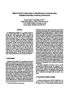
The Equi-Correlation Network algorithm was run with Gaussian RBFs on noisy samples of the sinc function, in order to visualize the functions that it minimizes, and illustrate the benefit of letting bandwidths of each Gaussian be automatically tuned. Fig. 1 represents the approximation obtained when the number of features in yˆ has reached 9, as well as each of these 9 features. First, one can notice that the approximation yˆ is very close to the function to approximate; second, we also notice that ECON actually uses kernels with different hyper-parameters. To exemplify the optimization of ξ, Fig. 2 shows the function that the algorithm has to minimize at the third iterations.

samples sinc approximation features

Figure 1: Approximation of noisy sinc after 12 steps, with 9 features. The dashed lines show these features, scaled by their weight in the network (ˆ y is represented by the bold line). Notice how the negative parts are approximated by means of a substraction of a large feature from a medium one.

5.1.2

The cos (exp ωx) function

The cos (exp ωx) is a toy problem in which we try to learn the function f (x) ≡ cos eωx + η, with x ∈ [0, 1], and η a noise with variance ση = 0.15. We set ω to 4 so that the function wiggles in the domain (see Fig. 3). This problem is used in [4]; it illustrates the fact that an algorithm is able, or not, to select useful parametrizations of the kernel. We stick to Guigue et al. experimental setting: the training set is made of 400 points drawn uniformly at random in [0, 1], and the test set is made of 1000 INRIA

13

The Equi-Correlated Network

3.5 3 2.5 2 1.5 1 0.5 0 0.5 0.4 0

0.3 0.2

0.4

0.2

bandwidth

0.1

0.6

0.8

center

1 0

Figure 2: Plot of the function to minimize at third step of sinc approximation: the z-axis represents the amount λ should decrease for the Gaussian with center x and bandwidth σ to appear in the LASSO solution. The peaks correspond to the active features in the current yˆ, for which this function is unfeasible (0/0).

points. In the training set, noise is added, whereas no noise is added in the test set. Fig. 3 shows very clearly that the fit is very good.

1

1.5 expected value predicted value

0.8 1 0.6 0.4 0.5 0.2 0

0

-0.2 -0.5 -0.4 -0.6 -1 -0.8 -1

-1.5 0

0.2

0.4

0.6

0.8

1

0

0.1

0.2

0.3

0.4

0.5

0.6

0.7

0.8

0.9

1

Figure 3: On the left, the cos-exp function to be learned. On the right, red points are the value to learn, while green points are the predictions. We see that the fit is quite very good.

5.1.3

Friedman’s functions

Friedman’s benchmark function were introduced in [2] and used quite widely. There are 3 such functions: F1 has P = 10 attributes, the domain being D = [0, 1]10 . The function is noisy, and 5 of the attributes are actually useless. F2 and F3 are defined on some subset of R4 and are also noisy. For each of these problems, we generate training sets made of 240 examples, and the same test set made of 1000 data1 . For these problems, we compare our results with those obtained by [12], on a LASSO algorithm (see table 1). The latter compares his own results with Support Vector Machine and Relevance Vector Machines. We measure the mean-squared error on the data-set: 1 To generate the data, we use the implementation available in R, in the mlbench package, with the standard setting for noise.

RR n° 6794

14

Loth Manuel and Preux Philippe

Table 1: We compare the performance of ECON with those published in [12], concerning the Support Vector Machine, the Relevance Vector Machine, and a LASSO-based algorithm proposed in this paper. For each algorithm, we provide the accuracy measured on a test set of 1000 data / K (aka, the number of support vectors) in yˆ, averaged over 100 runs for ECON. Both the average, and the median are provided. See the text for more discussion. F RIEDMAN ’ S FUNCTION

SVM MSE 2.92/116.2 4140/110.3 0.0202/106.5 AVE .

F1 F2 F3

Pn MSE =

i=1

RVM MSE 2.80/59.4 3505/6.9 0.0164/11.5 AVE .

[12] MSE 2.84/73.5 3808/14.2 0.0192/16.4 AVE .

AVE .

MSE 1.99/76 4845/54 0.0115/53

ECON M EDIAN MSE 1.97/71 4696/55 0.0113/53


2 yi − yˆ(xi ) n

Pn

where y¯ = i=1 yi /n. As ECON computes the whole regularization path, we compare the results obtained, in the same experimental settings, by ECON and the one proposed by [12] who obtains a solution with a certain number of terms in yˆ (K). On F1, ECON by far obtains the best results among the 4 algorithms. Only 17 terms provide an accuracy better than 2.8, the best accuracy mentioned for the other 3 algorithms. On F2, the results are less good, but are still rather good. To stick to the results published in [12], the figures in table 1 are averages; however, if we consider the best accuracy, or better, the histogram of accuracies, it is skewed towards better accuracies. On F3, we again obtain the best accuracy. It is also very significant to note that the number of kernels saturates at some point: on both F2, and F3, the mean number of kernels involved in yˆ is 54, with a standard deviation of 12. This saturation in the number of terms, while the test error keeps on decreasing, is a sign ECON does not overfit, or to the least, do not overfit a lot.

5.2

Real-world regression problems

To further the comparison, we use the well-known Boston housing dataset used by [4], as well as two datasets that are used in [12], namely abalone, and house-price-8L datasets2 . 5.2.1

Boston housing

This dataset is made of 502 data, each made of 13 attributes. We use the same experimental setting as [4] with which we compare our results: 20 % of the dataset as a test-set, the other 80 % being used for training. On 50 runs, we clearly outperform their results when using a single kernel, with an average accuracy on the test-set of 10.91, standard deviation of 3.56 (the distribution is very skewed, with more than half runs in the range 6-10, see Fig. 4). We note that on average, 232 basis functions are used (ranges from 100 to 400), that is about 25% less than Guigue et al. 2 For boston, we use the dataset from package mlbench, in R; for the other two, we use the datasets available at http://www.cs.toronto.edu/˜delve/delve.html.

INRIA

15

10 0

5

Frequency

15

The Equi-Correlated Network

10

15

20

MSE on test−set

Figure 4: Histogram of the best MSE measured on a test-set, obtained on 50 different runs. We see that the distribution is far from normal, so that the average, and standard deviation mentionned in the text only give a very poor image of the reality. Table 2: We compare the performance of ECON with those published in [12], concerning the Support Vector Machine, the Relevance Vector Machine, and a LASSO-based algorithm proposed in this paper. For Abalone, we provide the accuracy measured on a test set of 1000 data / the number of terms (aka, the number of support vectors) in yˆ, averaged on 100 runs for ECON. For house-price-8L, the training set is successively made of 1000, 2000, and 4000 data, the test set of 4000 data. See the text for more discussion. DATASET

A BALONE HOUSE - PRICE -8L, 1K HOUSE - PRICE -8L, 2K HOUSE - PRICE -8L, 4K

5.2.2

SVM 4.37/972 1.062/597 1.022/1307 1.012/2592

RVM 4.35/12 1.099/33 1.048/36 NA

[12] 4.35/19 1.075/61 1.054/63 1.024/69

ECON 4.31/71, 4.30/100 0.57/20 0.41/38 0.40/40

Abalone and house-price-8L

In both datasets, data are made of 8 attributes; Abalone holds 4177 data, while houseprice-8L has 22784 data. The results are provided in table 2. We see that ECON performs comparably to other methods on Abalone, much better than other methods on house-price-8L. Indeed, the accuracy of the test error is much better than the one published in [12], and the number of kernels is much smaller. As for Friedman’s functions, regarding the distribution of accuracies, the same remarks are true here again: for instance on Abalone, the best accuracy with 71 kernels is 4; on house-price-8L, we obtain much better performance, with often sparser expansions.

6

Conclusion and perspectives

In this paper, we considered the regression problem, for which we have proposed an algorithm, the Equi-Correlated Network, inspired by the (kernelized-)LARS. ECON automatically tunes the hyper-parameters of the kernel functions. The resulting algorithm can be seen as a non parametric one-hidden layer perceptron, that is, a perceptron RR n° 6794

16

Loth Manuel and Preux Philippe

in which the hidden layer does not contain a fixed amount of units, but grows according to the complexity of the problem to solve. Furthermore, building on the ability of the LARS to compute efficiently the whole l1 regularization path of the LASSO, ECON does not provide one solution, but the whole family of possible solution, according to the regularization parameter. This is a very interesting ability for practical purpose, and the fact that the algorithm is very efficient provides even more interest to ECON. Furthermore, sticking to this idea of closeness to MLPs, using a non parametric approach in which the hidden layer is not fixed, this let the estimator adapts to the complexity of the problem, to get the best compromise between under- and over-fitting, something an MLP with a fixed architecture can not achieve. There remains some work to do to fine tune ECON itself. The impact of the quality of the minimizations still has to be studied, both theoreticaly and experimentaly; some conditionning issues need to be clearly identified and solved; a good stopping criterion remains to be defined. It will also be important to investigate how this algorithm can be extended to more general loss and regularization functions, following the work of [11]. Finally, as pointed out in the introduction, ECON may be directly applied to classification problem, and this should be investigated, at least for an experimental assessment. Nevertheless, first experiments exhibits state-of-the-art performances on two realworld regression problems. These results were obtained without the need to set hyperparameters from domain knowledge, cross-validations, or high expertise in the algorithm. The key reason lies in the fact that although the class of models has a high expressivity, the optimization task in the space of all parameters is performed by a sequence of optimization in one feature’s parameters. As we are mostly interested in control optimization and sequential learning problems, further researches will focus on how this algorithm can be extended to online learning, moving targets, and specific ways to embed it in reinforcement learning algorithms.

References [1] B. Efron, T. Hastie, I. Johnstone, and R. Tibshirani. Least-angle regression. Annals of statistics, 32(2):407–499, 2004. [2] J. Friedman. Multivariate adaptive regression splines. 19(1):1–82, 1991.

Annals of Statistics,

[3] V. Guigue. M´ethodes a` noyaux pour la repr´esentation et la discrimination de signaux non-stationnaires. PhD thesis, Institut National des Sciences Appliqu´ees de Rouen, 2005. [4] V. Guigue, A. Rakatomamonjy, and S. Canu. Kernel basis pursuit. In Proc. ECML, volume 3720, pages 146–157. Springer, LNAI, 2005. [5] T. Hastie, R. Tibshirani, and J. Friedman. The elements of statistical learning — Data mining, inference and prediction. Statistics. Springer, 2001. [6] G-B. Huang, P. Saratchandran, and N. Sundararajan. A generalized growing and pruning RBF (GGAP-RBF) neural netowrk for function approximation. IEEE Transactions on Neural Networks, 16(1):57–67, January 2005.

INRIA

The Equi-Correlated Network

17

[7] D.R. Jones, C.D. Perttunen, and B.E. Stuckman. Lipschitzian optimization without the lipschitz constant. Journal of Optimization Theory and Aplications, 79(1):157–181, October 1993. [8] G. Kimeldorf and G. Wahba. Some results on tchebycheffian spline functions. J. Mathematical Analysis and Applications, 33(1):82–95, 1971. [9] S. Perkins, K. Lacker, and J. Theiler. Grafting: Fast, incremental feature selection by gradient descent in function space. Journal of Machine Learning Research, 3:1333–1356, 2003. [10] J. Platt. A resource-allocating network for function interpolation. Neural Computation, 3(2):213–225, 1991. [11] S. Rosset and J. Zhu. Piecewise linear regularized solution paths. Annals of Statistics, 35(3):1012–1030, 2007. [12] V. Roth. Generalizd lasso. IEEE Trans. on Neural Networks, 15(1):16–28, January 2004. [13] Sh. Shalev-Shwartz and N. Srebro. Low l1 norm and guarantees on sparsifiability, July 2008. Sparse Optimization and Variable Selection, Workshop, ICML/COLT/UAI. [14] R. Tibshirani. Regression shrinkage and selection via the lasso. J. Royal Statistics, 58(1):267–288, 1996. [15] S. Vijayakumar, A. D’Souza, and Stefan Schaal. Incremental online learning in high dimensions. Neural Computation, 17(12):2602–2632, 2002.

RR n° 6794

Unité de recherche INRIA Futurs Parc Club Orsay Université - ZAC des Vignes 4, rue Jacques Monod - 91893 ORSAY Cedex (France) Unité de recherche INRIA Lorraine : LORIA, Technopôle de Nancy-Brabois - Campus scientifique 615, rue du Jardin Botanique - BP 101 - 54602 Villers-lès-Nancy Cedex (France) Unité de recherche INRIA Rennes : IRISA, Campus universitaire de Beaulieu - 35042 Rennes Cedex (France) Unité de recherche INRIA Rhône-Alpes : 655, avenue de l’Europe - 38334 Montbonnot Saint-Ismier (France) Unité de recherche INRIA Rocquencourt : Domaine de Voluceau - Rocquencourt - BP 105 - 78153 Le Chesnay Cedex (France) Unité de recherche INRIA Sophia Antipolis : 2004, route des Lucioles - BP 93 - 06902 Sophia Antipolis Cedex (France)

Éditeur INRIA - Domaine de Voluceau - Rocquencourt, BP 105 - 78153 Le Chesnay Cedex (France)

http://www.inria.fr ISSN 0249-6399