Hindawi Publishing Corporation Journal of Applied Mathematics Volume 2014, Article ID 693659, 8 pages http://dx.doi.org/10.1155/2014/693659
Research Article The Extended Hamiltonian Algorithm for the Solution of the Algebraic Riccati Equation Zhikun Luo, Huafei Sun, and Xiaomin Duan School of Mathematics, Beijing Institute of Technology, Beijing 100081, China Correspondence should be addressed to Huafei Sun;
[email protected] Received 17 March 2014; Revised 27 April 2014; Accepted 8 May 2014; Published 20 May 2014 Academic Editor: Naseer Shahzad Copyright © 2014 Zhikun Luo et al. This is an open access article distributed under the Creative Commons Attribution License, which permits unrestricted use, distribution, and reproduction in any medium, provided the original work is properly cited. We use a second-order learning algorithm for numerically solving a class of the algebraic Riccati equations. Specifically, the extended Hamiltonian algorithm based on manifold of positive definite symmetric matrices is provided. Furthermore, this algorithm is compared with the Euclidean gradient algorithm, the Riemannian gradient algorithm, and the new subspace iteration method. Simulation examples show that the convergence speed of the extended Hamiltonian algorithm is the fastest one among these algorithms.
1. Introduction The algebraic Riccati equations (AREs) have been widely used in control system syntheses [1, 2], especially in optimal control [3], robust control [4], signal processing [5], and the LMI-based design [6]. And, in the past several decades, there has been an increasing interest in the solution problems of the AREs [7–9]. The lower matrix bounds for the AREs were discussed in [10, 11]. The structure-preserving doubling algorithm (SDA) was given under assumptions which are weaker than stabilizability and detectability, as well as practical issues involved in the application of the SDA to continuous-time AREs [12]. It is the purpose of this paper to investigate the unique (under suitable hypotheses) symmetric positive definite solution of an algebraic Riccati equation. Some effective methods, such as the Schur method (SM) [13] and the new subspace iteration method (NSIM) [14], were given for the numerical solution of the algebraic Riccati equation. Recently, the Euclidean gradient algorithm (EGA) and the Riemannian gradient algorithm (RGA) for the numerical solution of the algebraic Riccati equation with a cost function of the Riemannian distance on the curved Riemannian manifold were proposed in [15]. It is well known that the Euclidean gradient algorithm (EGA) and the Riemannian gradient algorithm (RGA) are first-order learning algorithms; hence the convergence speeds
of the EGA and RGA are very slow. The inclusion of a momentum term had been found to increase the rate of convergence dramatically [16, 17]. Based on this, the extended Hamiltonian algorithm (EHA) on manifolds was developed in [18], while its numerical implementation was discussed in [19]. Furthermore, the EHA is a second-order learning algorithm and converges faster than the first-order learning algorithm for optimization problem if certain conditions are satisfied. In this paper, we will apply the EHA to give the numerical solution of the AREs. Furthermore, we give two simulations to show the efficiency of our algorithm. Briefly, the rest of the paper is organized as follows. Section 2 is concluded with some fundamental knowledge on manifold that will be used throughout the paper. Section 3 introduces the extended Hamiltonian algorithm on manifold of positive definite symmetric matrices and Section 4 illustrates the convergence speeds of the EHA compared with other algorithms using two numerical examples. Section 5 concludes the paper.
2. Preliminaries In this section we recall some differential geometric facts of the space of positive definite symmetric matrices that will be used in the present analysis. More details can be found in [20– 23].
2
Journal of Applied Mathematics
2.1. The Frobenius Inner Product and the Euclidean Distance. Let 𝑀(𝑛) be the set of 𝑛 × 𝑛 real matrices and GL(𝑛) be its subset containing all the nonsingular matrices. GL(𝑛) is a Lie group, that is, a group which is also a differentiable manifold and for which the operations of group multiplication and inverse are smooth. The tangent space at the identity is called the corresponding Lie algebra denoted by gl(𝑛). It is the space of all linear transformations in R𝑛 , that is, 𝑀(𝑛). On 𝑀(𝑛), we use the Euclidean inner product, known as the Frobenius inner product and defined by ⟨𝑃, 𝑄⟩𝐹 = tr (𝑃𝑇 𝑄) ,
(1)
where tr stands for the trace of the matrix and superscript 𝑇 denotes the transpose. The associated norm ‖𝑃‖𝐹 = [tr(𝑃𝑇 𝑃)]1/2 is used to define the Euclidean distance on 𝑀(𝑛) by d𝐹 (𝑃, 𝑄) = ‖𝑃 − 𝑄‖𝐹 .
(2)
2.2. Geometry of Positive Definite Symmetric Matrices. We denote by Sym (𝑛) = {𝑠 ∈ 𝑀 (𝑛) | 𝑠 = 𝑠𝑇 }
(3)
(4)
the set of all 𝑛 × 𝑛 positive definite symmetric matrices, which is a differentiable manifold of dimension 𝑛(𝑛 + 1)/2. Here 𝑥 > 0 means the quadratic form 𝑧𝑇 𝑥𝑧 > 0 for all 𝑧 ∈ R𝑛 \ {0}. Furthermore, PD(𝑛) is an open convex cone; namely, if 𝑥1 and 𝑥2 are in PD(𝑛), so is 𝑥1 + 𝑡𝑥2 for any 𝑡 > 0. The exponential of any symmetric matrix is a positive definite symmetric matrix and the (principal) logarithm of any positive definite symmetric matrix is a symmetric matrix. Thus the exponential map from Sym(𝑛) to PD(𝑛) is one-to-one and onto. It follows that Sym(𝑛) provides a parameterization of PD(𝑛) via the exponential map. 2.3. Metric and Distances on PD(𝑛). Let 𝑔 denote the Riemannian metric on manifold PD(𝑛). For any 𝑥 ∈ PD(𝑛) the tangent space 𝑇𝑥 PD(𝑛) is identified with Sym(𝑛). On 𝑇𝑥 PD(𝑛) we define the inner product and the corresponding norm as follows: −1
−1
𝑔𝑥 (𝑢, V) = ⟨𝑢, V⟩𝑥 = tr (𝑥 𝑢𝑥 V) , 2
‖V‖𝑥 = [tr ((𝑥−1 V) )]
1/2
(5) ,
which depend on the point 𝑥. The positive definiteness of this metric is a consequence of the positive definiteness of the Frobenius inner product for 𝑔𝑥 (V, V) = ⟨V, V⟩𝑥 = tr (𝑥−1/2 V𝑥−1/2 𝑥−1/2 V𝑥−1/2 ) = ⟨𝑥−1/2 V𝑥−1/2 , 𝑥−1/2 V𝑥−1/2 ⟩ .
d𝐹 (𝑥1 , 𝑥2 ) = 𝑥1 − 𝑥2 𝐹 .
(7)
It will be more appropriate to use the Riemannian distance induced from (5), which is intrinsic to PD(𝑛) and defined by 1/2
𝑛 d𝑅 (𝑥1 , 𝑥2 ) = log (𝑥1−1/2 𝑥2 𝑥1−1/2 )𝐹 = (∑ln2 𝜆 𝑖 )
(6)
, (8)
𝑖=1
where 𝜆 𝑖 , 𝑖 = 1, 2, . . . , 𝑛, are the positive eigenvalues of 𝑥1−1 𝑥2 . The positivity of the 𝜆 𝑖 is a consequence of the similarity between the (in general nonsymmetric) matrix 𝑥1−1 𝑥2 and the positive definite symmetric matrix 𝑥1−1/2 𝑥2 𝑥1−1/2 . It is straightforward to see that the Riemannian distance (8) is invariant under inversion, that is, d𝑅 (𝑥1−1 , 𝑥2−1 ) = d𝑅 (𝑥1 , 𝑥2 )
the vector space of symmetric matrices and denote by PD (𝑛) = {𝑥 ∈ Sym (𝑛) | 𝑥 > 0}
Compared to manifold PD(𝑛) with the Frobenius inner product (1) resulting in a flat Riemannian manifold, manifold PD(𝑛) with the Riemannian metric (5) becomes a curved Riemannian manifold. To measure closeness of two positive definite symmetric matrices 𝑥1 and 𝑥2 one can use the Euclidean distance (2) of the ambient space 𝑀(𝑛); that is,
(9)
and is also invariant under congruent transformations; that is, d𝑅 (𝑥1 , 𝑥2 ) = d𝑅 (𝑃𝑇 𝑥1 𝑃, 𝑃𝑇 𝑥2 𝑃) ,
(10)
where 𝑃 ∈ GL(𝑛). Now, we discuss the geodesics on manifold PD(𝑛) under the different metrics. The geodesic passing through 𝑥 in the direction of V ∈ Sym(𝑛) with respect to the Euclidean metric (2) is given by 𝛾 (𝑡) = 𝑥 + 𝑡V,
0≤𝑡 0. The restriction that 𝑡 is not too large is necessary in order to ensure that the line stays within PD(𝑛). Similarly, the geodesic passing through 𝑥 in the direction of V ∈ Sym(𝑛) with respect to the Riemannian metric (5) is expressed by 𝛾 (𝑡) = 𝑥1/2 exp (𝑥−1/2 V𝑥−1/2 𝑡) 𝑥1/2 ,
(12)
which does not suffer the previous restriction. Let the exponential map Exp: Sym(𝑛) → PD(𝑛); then 𝑥2 = Exp𝑥1 (V) = 𝑥11/2 exp (𝑥1−1/2 V𝑥1−1/2 ) 𝑥11/2 .
(13)
Notice that the geodesic (12) is defined for all values of 𝑡, which is called geodesic completeness. The Hopf-Rinow theorem states that a geodesic complete manifold is also a complete metric space. And, manifold PD(𝑛) with the Riemannian metric (5) has nonpositive sectional curvature.
Journal of Applied Mathematics
3 distance functions (7) and (8), and the difference between 𝑄 and 𝑥𝐵𝑅−1 𝐵𝑇 𝑥 − 𝑥𝐴 − 𝐴𝑇 𝑥 can be expressed as follows:
3. The Extended Hamiltonian Algorithm for the Solution of AREs 3.1. Problem Formulation. The infinite time state regulator, namely, the state equation of linear time-invariant system, is in the form 𝑦̇ (𝑡) = 𝐴𝑦 (𝑡) + 𝐵𝑤 (𝑡) , 𝑛
𝑦 (𝑡0 ) = 𝑦0 ,
(14)
𝑚
where 𝑦(𝑡) ∈ R and 𝑤(𝑡) ∈ R are the state and the control vector, respectively, 𝐴 and 𝐵 are constant matrices of appropriate dimensions, and the terminal time 𝑡𝑓 = ∞. The problem would be to find an optimal control 𝑤(𝑡) satisfying (14) while minimizing the quadratic performance index as follows: 𝐽=
1 ∞ 𝑇 ∫ [𝑦 (𝑡) 𝑄𝑦 (𝑡) + 𝑤𝑇 (𝑡) 𝑅𝑤 (𝑡)] d𝑡, 2 0
(15)
where the designed parameters satisfy that both 𝑄 and 𝑅 are positive definite symmetric matrices. It has been proved that the optimal control 𝑤∗ (𝑡) of the cost function (15) is uniquely given by [24] 𝑤∗ (𝑡) = −𝑅−1 𝐵𝑇 𝑥𝑦 (𝑡)
(16)
and the quadratic optimal performance index is gotten by 1 𝐽∗ (𝑦 (𝑡0 )) = 𝑦𝑇 (𝑡0 ) 𝑥𝑦 (𝑡0 ) , 2
(17)
where 𝑥 is a positive definite symmetric matrix satisfying the AREs; that is, 𝑥𝐴 + 𝐴𝑇 𝑥 − 𝑥𝐵𝑅−1 𝐵𝑇 𝑥 + 𝑄 = 0.
(18)
It is assumed that the pair (𝐴, 𝐵) is completely controllable and that the pair (𝐴, 𝐷) is completely observable, where 𝐷𝐷𝑇 = 𝑄. Under these assumptions, (18) is known to have a unique positive definite solution 𝑥 [25]. There are, of course, other solutions to (18), but for the algorithm presented in this paper the emphasis will be on computing the positive definite one. Moreover, the optimal trajectory 𝑦(𝑡) satisfies the following optimal asymptotically stable closedloop system: 𝑦̇ (𝑡) = (𝐴 − 𝐵𝑅−1 𝐵𝑇 𝑥) 𝑦 (𝑡) = (𝐴 − 𝐵𝐾) 𝑦 (𝑡) ,
(19)
=
2 1 tr [(𝑄 + 𝑥𝐴 + 𝐴𝑇 𝑥 − 𝑥𝐵𝑅−1 𝐵𝑇 𝑥) ] , 2
(21)
1 𝐽𝑅 = d2𝑅 (𝑄, 𝑥𝐵𝑅−1 𝐵𝑇 𝑥 − 𝑥𝐴 − 𝐴𝑇 𝑥) 2 1 2 = log (𝑄−1/2 (𝑥𝐵𝑅−1 𝐵𝑇 𝑥 − 𝑥𝐴 − 𝐴𝑇 𝑥) 𝑄−1/2 )𝐹 2 =
1 tr {log2 [𝑄−1/2 (𝑥𝐵𝑅−1 𝐵𝑇 𝑥 − 𝑥𝐴 − 𝐴𝑇 𝑥) 𝑄−1/2 ]} . 2 (22)
Let 𝐽 : PD(𝑛) → R be a scalar function of 𝑛 × 𝑛 matrix. The Riemannian gradient of 𝐽 at 𝑥, denoted by ∇𝑥 𝐽, is a map from PD(𝑛) to Sym(𝑛) that satisfies ⟨∇𝑥 𝐽, 𝑠⟩𝑥 = ⟨𝜕𝑥 𝐽, 𝑠⟩𝐹 , for every 𝑠 ∈ Sym(𝑛), where 𝜕𝑥 𝐽 is the Euclidean gradient of 𝐽 at 𝑥. It follows from the inner product (5) that [27] ∇𝑥 𝐽 = 𝑥 (𝜕𝑥 𝐽) 𝑥.
(23)
Next, we will state some known facts, which are very helpful in computing 𝜕𝑥 𝐽𝐹 and ∇𝑥 𝐽𝑅 . Lemma 1 (see [28]). Let 𝐴, 𝐵 denote two constant matrices and let 𝑋, 𝑌 denote matrix functions. One has the following properties: (1) d tr (𝑋) = tr(d𝑋), (2) d(𝐴) = 0, (3) d(𝐴𝑋𝐵) = 𝐴(d𝑋)𝐵, (4) d(𝑋 ± 𝑌) = d𝑋 ± d𝑌, (5) d(𝑋𝑌) = (d𝑋)𝑌 + 𝑋(d𝑌), where d denotes the differential of a matrix (scalar) function. Lemma 2 (see [28]). Let 𝑓(𝑥) be a scalar function of 𝑛 × 𝑛 matrix 𝑥, if d𝑓 (𝑥) = tr (𝑊d𝑥)
(24)
𝜕𝑥 𝑓 (𝑥) = 𝑊𝑇 ,
(25)
holds; then where 𝜕𝑥 𝑓(𝑥) denotes the gradient of 𝑓(𝑥) and 𝑊 denotes the derivative of 𝑓(𝑥). Theorem 3. Let 𝐽𝐹 (𝑥) be a scalar function of 𝑛 × 𝑛 matrix 𝑥, if
where the state-feedback gain 𝐾 is given by 𝐾 = 𝑅−1 𝐵𝑇 𝑥.
1 𝐽𝐹 = d2𝐹 (𝑄, 𝑥𝐵𝑅−1 𝐵𝑇 𝑥 − 𝑥𝐴 − 𝐴𝑇 𝑥) 2
(20)
In order to solve (18), our purpose is to seek a matrix 𝑥 on manifold PD(𝑛) such that the matrix 𝑥𝐵𝑅−1 𝐵𝑇 𝑥 − 𝑥𝐴 − 𝐴𝑇 𝑥 is as close as possible to the given matrix 𝑄. 3.2. Distances and Gradients. In fact, the idea of formulating an equation on a manifold as a minimal-distance problem was suggested previously in [26]. Hence we use the two
𝐽𝐹 (𝑥) =
2 1 tr [(𝑄 + 𝑥𝐴 + 𝐴𝑇 𝑥 − 𝑥𝐵𝑅−1 𝐵𝑇 𝑥) ] 2
(26)
holds; then 𝜕𝑥 𝐽𝐹 (𝑥) = (𝐴 − 𝐵𝑅−1 𝐵𝑇 𝑥) (𝑄 + 𝑥𝐴 + 𝐴𝑇 𝑥 − 𝑥𝐵𝑅−1 𝐵𝑇 𝑥) + (𝑄 + 𝑥𝐴 + 𝐴𝑇 𝑥 − 𝑥𝐵𝑅−1 𝐵𝑇 𝑥) (𝐴𝑇 − 𝑥𝐵𝑅−1 𝐵𝑇 ) . (27)
4
Journal of Applied Mathematics
Proof. Since 𝑄+𝑥𝐴+𝐴𝑇 𝑥−𝑥𝐵𝑅−1 𝐵𝑇 𝑥 is symmetric, we have from Lemma 1 that
Proof. Since 𝑥𝐵𝑅−1 𝐵𝑇 − 𝑥𝐴 − 𝐴𝑇 𝑥 is symmetric, it follows immediately from Lemma 1 that
d𝐽𝐹 (𝑥) 2 1 = d {tr [(𝑄 + 𝑥𝐴 + 𝐴𝑇 𝑥 − 𝑥𝐵𝑅−1 𝐵𝑇 𝑥) ]} 2
=
d𝐽𝑅 (𝑥) 1 = d {tr log2 [𝑄−1/2 (𝑥𝐵𝑅−1 𝐵𝑇 𝑥 − 𝑥𝐴 − 𝐴𝑇 𝑥) 𝑄−1/2 ]} 2
2 1 tr [d(𝑄 + 𝑥𝐴 + 𝐴𝑇 𝑥 − 𝑥𝐵𝑅−1 𝐵𝑇 𝑥) ] 2
=
= tr [(𝑄 + 𝑥𝐴 + 𝐴𝑇 𝑥 − 𝑥𝐵𝑅−1 𝐵𝑇 𝑥) ×d (𝑄 + 𝑥𝐴 + 𝐴𝑇 𝑥 − 𝑥𝐵𝑅−1 𝐵𝑇 𝑥)]
1 tr {d log2 [𝑄−1/2 (𝑥𝐵𝑅−1 𝐵𝑇 𝑥 − 𝑥𝐴 − 𝐴𝑇 𝑥) 𝑄−1/2 ]} 2
= tr {log [𝑄−1/2 (𝑥𝐵𝑅−1 𝐵𝑇 𝑥 − 𝑥𝐴 − 𝐴𝑇 𝑥) 𝑄−1/2 ]
= tr [(𝑄 + 𝑥𝐴 + 𝐴𝑇 𝑥 − 𝑥𝐵𝑅−1 𝐵𝑇 𝑥)
×d log [𝑄−1/2 (𝑥𝐵𝑅−1 𝐵𝑇 𝑥 − 𝑥𝐴 − 𝐴𝑇 𝑥) 𝑄−1/2 ]}
× (d𝑥𝐴 + 𝐴𝑇 d𝑥 − d𝑥𝐵𝑅−1 𝐵𝑇 𝑥 − 𝑥𝐵𝑅−1 𝐵𝑇 d𝑥)]
= tr {log [𝑄−1/2 (𝑥𝐵𝑅−1 𝐵𝑇 𝑥 − 𝑥𝐴 − 𝐴𝑇 𝑥) 𝑄−1/2 ]
= tr {[(𝐴 − 𝐵𝑅−1 𝐵𝑇 𝑥) (𝑄 + 𝑥𝐴 + 𝐴𝑇 𝑥 − 𝑥𝐵𝑅−1 𝐵𝑇 𝑥)
× [𝑄−1/2 (𝑥𝐵𝑅−1 𝐵𝑇 𝑥 − 𝑥𝐴 − 𝐴𝑇 𝑥) 𝑄−1/2 ]
+ (𝑄 + 𝑥𝐴 + 𝐴𝑇 𝑥 − 𝑥𝐵𝑅−1 𝐵𝑇 𝑥)
−1
× 𝑄−1/2 d (𝑥𝐵𝑅−1 𝐵𝑇 𝑥 − 𝑥𝐴 − 𝐴𝑇 𝑥) 𝑄−1/2 }
× (𝐴𝑇 − 𝑥𝐵𝑅−1 𝐵𝑇 )] d𝑥} . (28)
= tr {log [𝑄−1/2 (𝑥𝐵𝑅−1 𝐵𝑇 𝑥 − 𝑥𝐴 − 𝐴𝑇 𝑥) 𝑄−1/2 ] −1
× (𝑥𝐵𝑅−1 𝐵𝑇 𝑥 − 𝑥𝐴 − 𝐴𝑇 𝑥)
Using the above Lemma 2, we have
× (d𝑥𝐵𝑅−1 𝐵𝑇 𝑥 − 𝑥𝐵𝑅−1 𝐵𝑇 d𝑥 − d𝑥𝐴 − 𝐴𝑇 d𝑥)}
𝜕𝑥 𝐽𝐹 (𝑥) = [ (𝐴 − 𝐵𝑅−1 𝐵𝑇 𝑥) (𝑄 + 𝑥𝐴 + 𝐴𝑇 𝑥 − 𝑥𝐵𝑅−1 𝐵𝑇 𝑥)
= tr {[(𝐵𝑅−1 𝐵𝑇 𝑥 − 𝐴) 𝑇
× log [𝑄−1/2 (𝑥𝐵𝑅−1 𝐵𝑇 𝑥 − 𝑥𝐴 − 𝐴𝑇 𝑥) 𝑄−1/2 ]
+ (𝑄 + 𝑥𝐴 + 𝐴𝑇 𝑥 − 𝑥𝐵𝑅−1 𝐵𝑇 𝑥) (𝐴𝑇 − 𝑥𝐵𝑅−1 𝐵𝑇 )]
−1
= (𝐴 − 𝐵𝑅−1 𝐵𝑇 𝑥) (𝑄 + 𝑥𝐴 + 𝐴𝑇 𝑥 − 𝑥𝐵𝑅−1 𝐵𝑇 𝑥)
× (𝑥𝐵𝑅−1 𝐵𝑇 𝑥 − 𝑥𝐴 − 𝐴𝑇 𝑥)
+ (𝑄 + 𝑥𝐴 + 𝐴𝑇 𝑥 − 𝑥𝐵𝑅−1 𝐵𝑇 𝑥) (𝐴𝑇 − 𝑥𝐵𝑅−1 𝐵𝑇 ) . (29)
− log [𝑄−1/2 (𝑥𝐵𝑅−1 𝐵𝑇 𝑥 − 𝑥𝐴 − 𝐴𝑇 𝑥) 𝑄−1/2 ] −1
× (𝑥𝐵𝑅−1 𝐵𝑇 𝑥 − 𝑥𝐴 − 𝐴𝑇 𝑥)
Therefore, it is shown that (27) is valid.
× (𝑥𝐵𝑅−1 𝐵𝑇 + 𝐴𝑇 )] d𝑥} .
Theorem 4. Let 𝐽𝑅 (𝑥) be a scalar function of 𝑛 × 𝑛 matrix 𝑥, if
(32)
1 𝐽𝑅 (𝑥) = tr {log2 [𝑄−1/2 (𝑥𝐵𝑅−1 𝐵𝑇 𝑥 − 𝑥𝐴 − 𝐴𝑇 𝑥) 𝑄−1/2 ]} 2 (30) Using the above Lemma 2, we have
holds; then ∇𝑥 𝐽𝑅 (𝑥)
𝜕𝑥 𝐽𝑅 (𝑥)
−1
= 𝑥 {(𝑥𝐵𝑅−1 𝐵𝑇 𝑥 − 𝑥𝐴 − 𝐴𝑇 𝑥) −1/2
× log [𝑄
−1 𝑇
−1 𝑇
𝑇
−1/2
(𝑥𝐵𝑅 𝐵 𝑥 − 𝑥𝐴 − 𝐴 𝑥) 𝑄
]
𝑇
× (𝑥𝐵𝑅 𝐵 − 𝐴 ) −1 𝑇
−1 𝑇
𝑇
−1
− (𝐵𝑅 𝐵 𝑥 + 𝐴) (𝑥𝐵𝑅 𝐵 𝑥 − 𝑥𝐴 − 𝐴 𝑥) −1/2
× log [𝑄
−1 𝑇
𝑇
−1/2
(𝑥𝐵𝑅 𝐵 𝑥 − 𝑥𝐴 − 𝐴 𝑥) 𝑄
] } 𝑥. (31)
= { (𝐵𝑅−1 𝐵𝑇 𝑥 − 𝐴) × log [𝑄−1/2 (𝑥𝐵𝑅−1 𝐵𝑇 𝑥 − 𝑥𝐴 − 𝐴𝑇 𝑥) 𝑄−1/2 ] −1
× (𝑥𝐵𝑅−1 𝐵𝑇 𝑥 − 𝑥𝐴 − 𝐴𝑇 𝑥)
− log [𝑄−1/2 (𝑥𝐵𝑅−1 𝐵𝑇 𝑥 − 𝑥𝐴 − 𝐴𝑇 𝑥) 𝑄−1/2 ] −1
× (𝑥𝐵𝑅−1 𝐵𝑇 𝑥 − 𝑥𝐴 − 𝐴𝑇 𝑥) (𝑥𝐵𝑅−1 𝐵𝑇 + 𝐴𝑇 )}
𝑇
Journal of Applied Mathematics
5 −1
= (𝑥𝐵𝑅−1 𝐵𝑇 𝑥 − 𝑥𝐴 − 𝐴𝑇 𝑥)
In order to apply (35) to solve (18), we plug (31) into (34) and get the final extended Hamiltonian algorithm on manifold PD(𝑛) as follows:
× log [𝑄−1/2 (𝑥𝐵𝑅−1 𝐵𝑇 𝑥 − 𝑥𝐴 − 𝐴𝑇 𝑥) 𝑄−1/2 ]
𝑥̇ = V,
× (𝑥𝐵𝑅−1 𝐵𝑇 − 𝐴𝑇 )
def
− (𝐵𝑅−1 𝐵𝑇 𝑥 + 𝐴) (𝑥𝐵𝑅−1 𝐵𝑇 𝑥 − 𝑥𝐴 − 𝐴𝑇 𝑥) −1/2
× log [𝑄
−1 𝑇
𝑇
−1/2
(𝑥𝐵𝑅 𝐵 𝑥 − 𝑥𝐴 − 𝐴 𝑥) 𝑄
× log [𝑄−1/2 (𝑥𝐵𝑅−1 𝐵𝑇 𝑥 − 𝑥𝐴 − 𝐴𝑇 𝑥) 𝑄−1/2 ] , (38)
]. (33)
Combining (23) and (33), (31) is established. This completes the proof of Theorem 4. 3.3. The Extended Hamiltonian Algorithm on 𝑃𝐷(𝑛). The Euclidean gradient algorithm (EGA) and the Riemannian gradient algorithm (RGA) are first-order learning algorithms and inherit some drawbacks that are well known about gradient-based optimization like, for instance, the slowlearning phenomenon in presence of plateau in the error surface. In order to overcome this difficulty, Fiori generalized EGA and RGA and proposed the extended Hamiltonian algorithm on manifold. In particular, on manifold PD(𝑛), the extended Hamiltonian algorithm can be expressed by [18] 𝑥̇ = V, −1
V̇ = V𝑥 V − ∇𝑥 𝑉 − 𝜇V,
(34)
where 𝑥 ∈ PD(𝑛), V denotes the instantaneous learning velocity, 𝑉 : PD(𝑛) → R denotes a cost function, ∇𝑥 𝑉 denotes the Riemannian gradient of 𝑉, and the constant 𝜇 > 0 denotes a viscosity term. The function 𝐾𝑥 : 𝑇𝑥 PD(𝑛) × 𝑇𝑥 PD(𝑛) → R denotes the kinetic energy of the particle in a point 𝑥 and has the corresponding expression 𝐾𝑥 = (1/2) tr[(V𝑥−1 )2 ]. System (34) may be implemented by [19] 𝑥𝑘+1 = 𝑥𝑘1/2 exp (𝜂𝑥𝑘−1/2 V𝑘 𝑥𝑘−1/2 ) 𝑥𝑘1/2 , V𝑘+1 = 𝜂 [V𝑘 𝑥𝑘−1 V𝑘 − ∇𝑥𝑘 𝑉] + (1 − 𝜂𝜇) V𝑘 ,
(35)
where 𝜂 is a small positive number known as the learning rate. The effectiveness of the algorithm is ensured if and only if √2𝜆 max < 𝜇
0 denotes the learning rate and the constant 𝜇 denotes a viscosity term. Now, based on the above discussion, we give the iterative formula of the EHA for the numerical solution of (18). Algorithm 5 (EHA). For any 𝑥 belonging to the considered manifold PD(𝑛), the extended Hamiltonian algorithm is given by the following. (1) Set 𝑥0 as an initial input matrix 𝑥 and V0 as an initial direction of V, and then choose a desired tolerance 𝜀 > 0. (2) Compute 𝑉(𝑥𝑘 ). (3) If 𝑉(𝑥𝑘 ) < 𝜀 then stop. (4) Update 𝑥 and V by (39) and return to step (2).
4. Simulations In this section, we give two computer simulations to demonstrate the effectiveness and performance of the proposed algorithm. Example 1. First consider a second-order algebraic Riccati equation. In the present experiment, 𝜂 = 0.01, 𝜇 = 3, and 𝜀 = 10−8 . Moreover, 𝐴, 𝐵, 𝑄, 𝑅, and 𝐷 used in this simulation are as follows: 0 0 1 𝐴=( ), 𝐵 = ( ), 1 0 0 (40) √2 0 1 2 0 ), 𝐷=( 𝑄=( ), 𝑅= , 0 2 0 √2 2 which satisfy the unique definite solution condition.
6
Journal of Applied Mathematics 0.7
×10−3 4
0.6
3.5 3
0.4
Kinetic function
Cost function
0.5
0.3 0.2
2 1.5 1
0.1 0
2.5
0.5 0
10
20
EGA NSIM
30
40 50 Iterations
60
70
80
90
0
0
RGA EHA
5
10
15 Iterations
20
25
30
100
120
Figure 2: Kinetic energy in the EHA.
Figure 1: Comparison of convergence speeds of the EGA, the RGA, the NSIM, and the EHA.
1 0.9 0.8
(
1.4142136 0.9999999 ). 1.0000000 2.8284271
(41)
0.7 Cost function
To study the performance differences among the EHA, the EGA, the RGA, and the NSIM, these algorithms are, respectively, applied to solve (18). In this paper, the optimal step size 𝜂, which corresponds to the best convergence speed in each algorithm, is obtained by numerical experiments. For instance, it can be found that the iterations will reduce gradually as the step size changes from 0.01 to 0.1, while the algorithm will be divergent once the step size is bigger than 0.1. Thus this optimal step size 𝜂 is convenient to be obtained experimentally. Based on (36), the constant 𝜇 > 0 depends on the selection of initial value. That is to say, different initial values will be corresponding to different 𝜇; hence the best 𝜇 is also obtained by the experiment. As Figure 1 shows, the behavior of the cost function is shown. Clearly, in the early stages of learning, the EHA decreases much faster than the EGA, the RGA, and the NSIM with the same learning step size. The result shows that the EHA has the fastest convergence speed among four algorithms and needs 28 iterations to obtain the numerical solution of the ARE as follows:
0.6 0.5 0.4 0.3 0.2 0.1 0
0
20
40
60 Iterations
EGA NSIM
80 RGA EHA
Figure 3: Comparison of convergence speeds of the EGA, the RGA, the NSIM, and the EHA.
0 1 0 𝐴 = (1 0 1) , 0 1 0 1 0 0 𝑄 = (0 1 0) , 0 0 1
𝑅 = 1,
1 𝐵 = (0) , 0 1 0 0 𝐷 = (0 1 0) . 0 0 1
(42)
However, RGA realizes the given error through 36 iterations and the slowest one among them is the EGA with 88 steps. And Figure 2 shows that the kinetic energy function finally converges to 0.
As Figure 3 shows, the convergence speed of the EHA is still the fastest one among four algorithms. Finally, we get the numerical solution of the ARE as follows:
Example 2. A third-order ARE is considered following the similar procedure as Example 1. In this experiment, 𝜂 = 0.01, 𝜇 = 2.5, and 𝜀 = 10−8 , and
3.6502815 6.1622776 5.0644951 (6.1622776 13.7792717 12.3245553) . 5.0644951 12.3245553 12.3650582
(43)
Journal of Applied Mathematics
7
×10−3 4 3.5
Kinetic function
3 2.5 2 1.5 1 0.5 0
5
0
10
15 Iterations
20
25
30
Figure 4: Kinetic energy in the EHA.
Moreover, the kinetic energy function also converges to 0 in the Figure 4.
5. Summary In this paper, a second-order learning method called the extended Hamiltonian algorithm is recalled from literature and applied to solve the numerical solution for the algebraic Riccati equation. And, the convergence speed of the provided algorithm is compared with the EGA, the RGA, and the NSIM using two simulation examples. It is shown that the convergence speed of the extended Hamiltonian algorithm is the fastest one among these algorithms.
Conflict of Interests The authors declare that there is no conflict of interests regarding the publication of this paper.
Acknowledgments This subject is supported by the National Natural Science Foundations of China (nos. 61179031 and 10932002).
References [1] K. Zhou, J. Doyle, and K. Glover, Robust and Optimal Control, Prentice Hall, Upper Saddle River, NJ, USA, 1996. [2] Z. Lin, “Global control of linear systems with saturating actuators,” Automatica, vol. 34, no. 7, pp. 897–905, 1998. [3] D.-Z. Zheng, “Optimization of linear-quadratic regulator systems in the presence of parameter Perturbations,” IEEE Transactions on Automatic Control, vol. 31, no. 7, pp. 667–670, 1986. [4] M. L. Ni and H. X. Wu, “A Riccati equation approach to the design of linear robust controllers,” Automatica, vol. 29, no. 6, pp. 1603–1605, 1993.
[5] T. Kaneko, S. Fiori, and T. Tanaka, “Empirical arithmetic averaging over the compact Stiefel manifold,” IEEE Transactions on Signal Processing, vol. 61, no. 4, pp. 883–894, 2013. [6] H.-P. Liu, F.-C. Sun, K.-Z. He, and Z.-Q. Sun, “Simultaneous stabilization for singularly perturbed systems via iterative linear matrix inequalities,” Acta Automatica Sinica, vol. 30, no. 1, pp. 1– 7, 2004. [7] V. Sima, Algorithms for Linear-Quadratic Optimization, vol. 200 of Monographs and Textbooks in Pure and Applied Mathematics, Marcel Dekker, New York, NY, USA, 1996. [8] P. Benner, J.-R. Li, and T. Penzl, “Numerical solution of large-scale Lyapunov equations, Riccati equations, and linearquadratic optimal control problems,” Numerical Linear Algebra with Applications, vol. 15, no. 9, pp. 755–777, 2008. [9] H. G. Xu and L. Z. Lu, “Properties of a quadratic matrix equation and the solution of the continuous-time algebraic Riccati equation,” Linear Algebra and Its Applications, vol. 222, pp. 127–145, 1995. [10] H. H. Choi and T.-Y. Kuc, “Lower matrix bounds for the continuous algebraic Riccati and Lyapunov matrix equations,” Automatica, vol. 38, no. 8, pp. 1147–1152, 2002. [11] R. Davies, P. Shi, and R. Wiltshire, “New lower solution bounds of the continuous algebraic Riccati matrix equation,” Linear Algebra and Its Applications, vol. 427, no. 2-3, pp. 242–255, 2007. [12] E. K.-W. Chu, H.-Y. Fan, and W.-W. Lin, “A structure-preserving doubling algorithm for continuous-time algebraic Riccati equations,” Linear Algebra and Its Applications, vol. 396, pp. 55–80, 2005. [13] A. J. Laub, “A Schur method for solving algebraic Riccati equations,” IEEE Transactions on Automatic Control, vol. 24, no. 6, pp. 913–921, 1979. [14] Y. Lin and V. Simoncini, “A new subspace iteration method for the algebraic Riccati equation,” preprint, http://arxiv.org/ abs/1307.3843. [15] X. Duan, Information geometry of matrix Lie groups and applications [Ph.D. thesis], Beijing Institute of Technology, 2013, (Chinese). [16] D. Rumelhart and J. McClelland, Parallel Distributed Processing, MIT Press, 1986. [17] N. Qian, “On the momentum term in gradient descent learning algorithms,” Neural Networks, vol. 12, no. 1, pp. 145–151, 1999. [18] S. Fiori, “Extended Hamiltonian learning on Riemannian manifolds: theoretical aspects,” IEEE Transactions on Neural Networks, vol. 22, no. 5, pp. 687–700, 2011. [19] S. Fiori, “Extended Hamiltonian learning on Riemannian manifolds: numerical aspects,” IEEE Transactions on Neural Networks and Learning Systems, vol. 23, no. 1, pp. 7–21, 2012. [20] M. Moakher, “A differential geometric approach to the geometric mean of symmetric positive-definite matrices,” SIAM Journal on Matrix Analysis and Applications, vol. 26, no. 3, pp. 735–747, 2005. [21] M. Moakher, “On the averaging of symmetric positive-definite tensors,” Journal of Elasticity, vol. 82, no. 3, pp. 273–296, 2006. [22] A. Schwartzman, Random ellipsoids and false discovery rates: statistics for diffusion tensor imaging data [Ph.D. thesis], Stanford University, 2006. [23] J. Jost, Riemannian Geometry and Geometric Analysis, Universitext, Springer, Berlin, Germany, Third edition, 2002. [24] R. E. Kalman, “Contributions to the theory of optimal control,” Boletin de la Sociedad Matematica Mexicana, vol. 5, no. 2, pp. 102–119, 1960.
8 [25] R. Kalman, “When is a linear control system optimal?” Journal of Basic Engineering, vol. 86, no. 1, pp. 51–60, 1964. [26] S. Fiori, “Solving minimal-distance problems over the manifold of real-symplectic matrices,” SIAM Journal on Matrix Analysis and Applications, vol. 32, no. 3, pp. 938–968, 2011. [27] R. Greg´orio and P. Oliveira, “A proximal technique for computing the Karcher mean of symmetric positive definite matrices,” Optimization Online, 2013. [28] X. Zhang, Matrix Analysis and Application, Springer, New York, NY, USA, 2004.
Journal of Applied Mathematics
Advances in
Operations Research Hindawi Publishing Corporation http://www.hindawi.com
Volume 2014
Advances in
Decision Sciences Hindawi Publishing Corporation http://www.hindawi.com
Volume 2014
Journal of
Applied Mathematics
Algebra
Hindawi Publishing Corporation http://www.hindawi.com
Hindawi Publishing Corporation http://www.hindawi.com
Volume 2014
Journal of
Probability and Statistics Volume 2014
The Scientific World Journal Hindawi Publishing Corporation http://www.hindawi.com
Hindawi Publishing Corporation http://www.hindawi.com
Volume 2014
International Journal of
Differential Equations Hindawi Publishing Corporation http://www.hindawi.com
Volume 2014
Volume 2014
Submit your manuscripts at http://www.hindawi.com International Journal of
Advances in
Combinatorics Hindawi Publishing Corporation http://www.hindawi.com
Mathematical Physics Hindawi Publishing Corporation http://www.hindawi.com
Volume 2014
Journal of
Complex Analysis Hindawi Publishing Corporation http://www.hindawi.com
Volume 2014
International Journal of Mathematics and Mathematical Sciences
Mathematical Problems in Engineering
Journal of
Mathematics Hindawi Publishing Corporation http://www.hindawi.com
Volume 2014
Hindawi Publishing Corporation http://www.hindawi.com
Volume 2014
Volume 2014
Hindawi Publishing Corporation http://www.hindawi.com
Volume 2014
Discrete Mathematics
Journal of
Volume 2014
Hindawi Publishing Corporation http://www.hindawi.com
Discrete Dynamics in Nature and Society
Journal of
Function Spaces Hindawi Publishing Corporation http://www.hindawi.com
Abstract and Applied Analysis
Volume 2014
Hindawi Publishing Corporation http://www.hindawi.com
Volume 2014
Hindawi Publishing Corporation http://www.hindawi.com
Volume 2014
International Journal of
Journal of
Stochastic Analysis
Optimization
Hindawi Publishing Corporation http://www.hindawi.com
Hindawi Publishing Corporation http://www.hindawi.com
Volume 2014
Volume 2014