The Extended Partitioning Problem: Hardware/Software ... - CiteSeerX

—— Submitted to —— Journal of Design Automation of Embedded Systems, special issue, “System Partitioning Issues”

T Y• O F•

SI

C

E

A

R

E BE

•

ER

I

T

H

A

NIV

T

H

ORN

L IG H T

LE

E•U

LIF

A

•1868•

The Extended Partitioning Problem: Hardware/Software Mapping, Scheduling, and Implementation-bin Selection

•T

Department of Electrical Engineering and Computer Sciences University of California Berkeley, California 94720

Asawaree Kalavade Edward A. Lee

Abstract In system-level design, applications are represented as task graphs where tasks (called nodes) have moderate to large granularity and each node has several implementation options differing in area and execution time. We define the extended partitioning problem as the joint determination of the mapping (hardware or software), the implementation option (called implementation bin), as well as the schedule, for each node, so that the overall area allocated to nodes in hardware is minimum and a deadline constraint is met. This problem is considerably harder (and richer) than the traditional binary partitioning problem that determines just the best mapping and schedule. Both binary and extended partitioning problems are constrained optimization problems and are NP-hard. We first present an efficient (O(N2)) heuristic, called GCLP, to solve the binary partitioning problem. The heuristic reduces the greediness associated with traditional list-scheduling algorithms by formulating a global measure, called global criticality (GC). The GC measure also permits an adaptive selection of the optimization objective at each step of the algorithm; since the optimization problem is constrained by a deadline, either area or time is optimized at a given step based on the value of GC. The selected objective is used to determine the mapping of nodes that are “normal”, i.e. nodes that do not exhibit affinity for a particular mapping. To account for nodes that are not “normal”, we define “extremities” and “repellers”. Extremities consume disproportionate amounts of resources in hardware and software. Repellers are inherently unsuitable to either hardware or software based on certain structural properties. The mapping of extremities and repellers is determined jointly by GC and their local preference. We then present an efficient (O(N3 + N2B), for N nodes and B bins per node) heuristic for extended partitioning, called MIBS, that alternately uses GCLP and an implementation-bin selection procedure. The implementation-bin selection procedure chooses, for a node with already determined mapping, an implementation bin that maximizes the area-reduction gradient of as-yet unmapped nodes. Solutions generated by both heuristics are shown to be reasonably close to optimal. Extended partitioning generates considerably smaller overall hardware as compared to binary partitioning. This research is part of the Ptolemy project, which is supported by the Advanced Research Projects Agency and the U.S. Air Force (under the RASSP program F33615-93-C-1317), the Semiconductor Research Corporation (SRC) (project 95-DC-324016), the National Science Foundation (MIP-9201605), the State of California MICRO program, and the following companies: Bell Northern Research, Cadence, Dolby, Hitachi, Lucky-Goldstar, Mentor Graphics, Mitsubishi, Motorola, NEC, Philips, and Rockwell. 1 of 40

Introduction

1.0

Introduction System-level design usually involves designing an application specified at a large granularity. A typ-

ical design objective is to minimize cost (in terms of area or power) while the performance constraints are usually throughput or latency requirements. The basic component of the system-level specification is called a task or a node. The key issues in system-level design are partitioning, synthesis, simulation, and design methodology management. The partitioning process determines an appropriate hardware or software mapping and an implementation for each node, given several hardware and software implementation options for every node in the task-level specification. A partitioned application has to be synthesized and simulated within a unified framework that involves the hardware and software components as well as the generated interfaces. The system-level design space is quite large and the system-level design problem cannot, in general, be posed as a single well-defined optimization problem. Typically, the designer needs to explore the possible options, tools, and architectures. A design methodology management framework helps to manage the design space exploration process. We have developed a software environment, called the Design Assistant, that addresses all these issues [1]. The Design Assistant consists of: (1) specific tools for partitioning, synthesis, and simulation that are configured for a particular hardware-software codesign flow, and (2) an underlying design methodology management infrastructure for design space exploration. In this paper we will focus on the partitioning problem. A very important aspect of system-level design is the multiplicity of design options available for every node in the task-level specification. Each node can be implemented in several ways in both hardware and software mappings. The partitioning problem is to select an appropriate combination of mapping and implementation for each node. For instance, a given task can be implemented in hardware using design options at several levels. 1. Algorithm level: Several algorithms can be used to describe the same task. For instance, a finite impulse response filter can be implemented either as an inner product or using the FFT in a shiftand-add algorithm. Figure 1 shows the direct and transform forms for a biquad. 2. Transformation level: For a particular algorithm, several transformations [2] can be applied on the original task description. Figure 1-b shows two such transformations. 3. Resource level: A task, for a specified algorithm and transformation set, can be implemented using varying numbers of resource units. Figure 1-c shows two resource-level implementation options for The Extended Partitioning Problem

2 of 40

Introduction

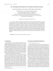
the direct form biquad. A particular task can thus be implemented in several ways. To illustrate this further, Figure 2 shows the Pareto-optimal points in the area-time trade-off curves for the hardware implementation of typical nodes. The sample period is shown on the X axis, and the corresponding hardware area required to implement the node is shown on the Y axis. The left-most point on the X axis for each curve corresponds to the fastest possible implementation of the node. The right-most point on the X axis for each curve corresponds to the smallest possible area. Thus, the curve represents the design space for the task in a hardware mapping1. Similarly, different software synthesis strategies can be used to implement a given node Task (Biquad) (a) Algorithm-level implementation options

D

D D

D

Direct form Transpose form (b) Transformation-level implementation options

a3

a4

a3 m1

m3

D

a1

a1

a2 D

m2

m4

cycle operations

# adders = 2

1

# multipliers = 2

2 3 4

area = 22

s1 D >> s2 D >>

s3 >> s4 >>

a2

a3

a4 D m1

tc = 4 cycles

m1 m2 m3 m4 a1

# adders = 2

a3 a2 a4

area = 10

# add/shift = 2

s3 s4 a1 a3 a2 a4

a2

D m2 D

cycle operations 1 s1 s2 2 3 4

m3

a1

replace multiply by shift-add

original tc = 4 cycles

a4

m4 D

retimed tc = 4 cycles # adders = 1 # multipliers = 1 area = 11

cycle operations 1 m1 a3 2 m2 a2 3 4

m3 a1 m4 a4

(amultiply = 10 aadd = 1 ashift-add = 3) (tmultiply = tadd = tshift-add = 1 cycle)

in m1

m2 a1

in

m3

m4

a2

a3

a4 out Corresponding Control-dataflow graph

(c) Resource-level implementation options ops cycle m1 m2 1 m3 m4 a1 2 a3 a2 3 a4 4

t = 4 cycles a = 22

Fastest implementation

cycle ops m1 1 m2 2 m3 a1 3 m4 a3 4 a2 5 a4 6

t = 6 cycles a = 11

Smallest implementation Figure 1.

The Extended Partitioning Problem

Hardware design options for a “node”.

3 of 40

Introduction

in software. For instance, inlined code is faster than code using subroutine calls, but has a larger code size. Thus, there is a trade-off between code size and execution time. In summary, each node in the task-level description can be implemented in several ways in either hardware or software. It is not sufficient to just determine whether a node is to be mapped to hardware or software — the appropriate implementation needs to be determined as well. A system-level specification consists of a number of tasks and the goal is to optimize the overall design. Clearly, it is not enough to optimize each task independently. For example, if each task in the task-level specification were fed to a high-level hardware synthesis tool that is optimized for speed (i.e., generates the fastest implementation), then the overall area of the system might be too large. Thus, a mapping and implementation that optimizes the overall design should be selected for each node. In addition to mapping and implementation selection, a third aspect of partitioning is to schedule the application i.e., determine when each node executes. Scheduling after fixing a mapping and implementation leaves little flexibility in meeting the timing constraints; hence scheduling should be done simultaneously with mapping and implementation selection.

65 pulse_shaper

60

fastest bin for equalizer node timing_recovery equalizer

55

hardware area

50 45 40

implementation bins for pulse_shaper

35 30 25 20

slowest bin for equalizer node

15 10 0

Figure 2.

20

40

60

80

100

sample period (cycles) Typical hardware implementation curves.

120

1. We generated each of these curves by running a task-level Silage [3] description of the node through Hyper [4].


4 of 40

Introduction

Thus, the goal of partitioning is to determine three parameters for each task: mapping (hardware or software), implementation ( type of implementation to use with respect to the algorithm, transformation, and area-time value), and schedule (when it executes, relative to other tasks). Partitioning is a non-trivial problem. Consider a task-level specification, typically in the order of 50 to 100 tasks. Each task can be mapped to either hardware or software. Furthermore, within a given mapping, a task can be implemented in one of several options, as shown in Figure 2. Suppose there are 5 design options for each node. Thus there are (2*5)100 design options in the worst case! Although a designer may have a preferred implementation for some (say p) nodes, there is still a large number of design alternatives with respect to the remaining nodes ((2*5)100-p). Determining the best design option for all the nodes is, in fact, a constrained optimization problem. The design parameters can often be used to formulate this problem as an integer optimization problem. Exact solutions to such formulations (typically using integer linear programming (ILP)) are intractable for even moderately small problems. In this paper, we propose and evaluate heuristic solutions. The heuristics will be shown to be comparable to the ILP solution in quality, with a much reduced solution time. We study the partitioning problem in two stages, binary partitioning and extended partitioning. Binary partitioning is the problem of determining, for each node, a hardware or a software mapping and a schedule. Extended partitioning is the problem of selecting an appropriate implementation, over and above binary partitioning. Currently published approaches on hardware/software partitioning focus only on the binary partitioning problem; one of the contributions of this work is the formulation of the extended partitioning problem. Before we formally define these two problems, we digress briefly to outline the key assumptions in our work. Assumptions System-level design is a very broad problem. We restrict our attention to the design of embedded systems with real-time signal processing components. Examples of such systems include modems for both tethered and wireless communication, cordless phones, disk drive controllers, printers, digital audio systems, data compression systems, etc. The partitioning techniques discussed in this paper are based on the following assumptions: 1. The precedences between the tasks are specified as a directed acyclic graph (DAG G = (N, A))2. The throughput constraint on the graph translates to a deadline D, i.e., the execution time of the DAG 2. Such a DAG can be generated from a synchronous dataflow (SDF) graph, which allows loops and multirate operations, thus making it possible to represent a reasonably large class of applications [5].


5 of 40

Introduction

should not exceed D clock cycles. 2. The target architecture consists of a single programmable processor (which executes the software component) and a custom datapath (the hardware component). The software and hardware components have capacity constraints — the software (program and data) size should not exceed AS (memory capacity) and the hardware size should not exceed AH. The communication costs of the hardware-software interface are represented by three parameters: ahcomm, ascomm, and tcomm. Here, ahcomm (ascomm) is the hardware (software) area required to communicate one sample of data across the hardware-software interface and tcomm is the number of cycles required to transfer the data. The parameter ahcomm represents the area of the interface glue logic and ascomm represents the size of the code that sends or receives the data. In our implementation we assume a self-timed blocking memory-mapped interface. We neglect the communication costs of software-to-software and hardwareto-hardware interfaces. 3. The area and time estimates for the hardware and software implementation bins of every node are assumed to be known. We assume that, associated with every node i, is a hardware implementation curve CHi, and a software implementation curve CSi. The implementation curve plots all the possible design alternatives (referred to as implementation bins) for the node. CHi = {(ahij, thij), j ∈ NH }, where ahij and thij represent the area and execution time when node i is implemented in i hardware bin j, and NHi is the set of all the hardware implementation bins. CSi = {(asij, tsij), j ∈ NS }, where asij and tsij represent the program size and execution time when node i is implei mented in software bin j, and NSi is the set of all the software implementation bins. Within a mapping, the fastest implementation bin is called L bin, and the slowest implementation bin is called H bin. In the case of binary partitioning, where a single implementation bin is assumed, ahi, thi, asi, and tsi represent the area and execution time in hardware and software respectively. The specific techniques used to estimate these values are described in Section 4.0. 4. We assume that there is no reuse between nodes mapped to hardware. Problem Definition The binary partitioning problem (P1): Given a DAG, area and time estimates for software and hardware mappings of all nodes, and communication costs, subject to resource capacity constraints and a deadline D, determine for each node i, the hardware or software mapping (Mi) and the start time for the execution of the node (schedule ti), such that the total area occupied by the nodes mapped to hardware is minimum. P1 is NP-hard and can be formulated exactly as an ILP [1]. The Extended Partitioning Problem

6 of 40

Related Work

The extended partitioning problem (P2): Given a DAG, hardware and software implementation curves for all the nodes, communication costs, resource capacity constraints, and a required deadline D, find a hardware or software mapping (Mi), the implementation bin (Bi*), and the schedule (ti) for each node i, such that the total area occupied by the nodes mapped to hardware is minimum. It is obvious that P2 is a much harder problem than P1. It has (2B)|N| alternatives, given B implementation bins per mapping. P2 can be formulated exactly as an integer linear program, similar to P1. An ILP formulation for P2 is given in [1]. The motivation for solving the extended partitioning problem is two-fold. First, the flexibility of selecting an appropriate implementation bin for a node, instead of assuming a fixed implementation, is likely to reduce the overall hardware area. In this paper, we investigate, with examples, the pay-off in using extended partitioning over just mapping (binary partitioning). Secondly, from the practical perspective of hardware (or software) synthesis, solution to P2 provides us with the best sample period or algorithm to use for the synthesis of a given node. The rest of the paper is organized as follows. In Section 2.0, we discuss some of the related work in the area of hardware/software partitioning. In Section 3.0, we present the GCLP algorithm to solve the binary partitioning problem. Its performance is analyzed in Section 4.0. In Section 5.0, we present the MIBS heuristic to solve the extended partitioning problem. The MIBS algorithm essentially solves two problems for each node in the precedence graph: hardware/software mapping and scheduling, followed by implementation-bin selection for this mapping. The first problem, that of mapping and scheduling, is solved by the GCLP algorithm. For a given mapping, an appropriate implementation bin is selected using a bin selection procedure. The bin selection procedure is described in Section 6.0. The details of the MIBS algorithm are described in Section 7.0, and its performance is analyzed in Section 8.0.

2.0

Related Work Binary Partitioning Gupta et al. [6] discuss a scheme where all data-independent nodes are initially mapped to hardware.

Nodes are at an instruction level of granularity. Nodes are progressively moved from hardware to software if the resultant solution is feasible and the cost of the new partition is smaller than the earlier cost. The scheme proposed by Henkel et al. [7] also assumes an instruction level of granularity. All the nodes are mapped to software at the start and then moved to hardware (using simulated annealing) until timing


7 of 40

Related Work

constraints are met. Baros et al. [8] present a two-stage clustering approach to the mapping problem. Clusters are characterized by attribute values and are assigned hardware and software mappings based on their attribute values. D’Ambrosio et al. [9] describe an approach for partitioning applications where each node has a deadline constraint. The input specification is transformed into a set of constraints that is solved by an optimizing tool called GOPS, which uses a branch and bound approach, to determine the mapping. Thomas et al. [10] propose a manual partitioning approach for task-level specifications. They discuss the properties of tasks that render them suitable to either hardware or software mapping. In their approach, the designer has to qualitatively evaluate these properties and make a mapping decision. Next, we briefly discuss some work in related areas such as software partitioning, hardware partitioning, and high-level synthesis to evaluate the possibility of extending it to the binary partitioning problem. The heterogeneous multiprocessor scheduling problem is to partition an application into multiple heterogeneous processors. Approaches used in the literature [11][12] to solve this problem ignore the area dimension while selecting the mapping; they cannot be directly applied to the hardware/software mapping and scheduling problem. Considerable attention has been directed towards the hardware partitioning problem in the high-level hardware synthesis community. The goal in most cases is to meet the chip capacity constraints; timing constraints are not considered. Most of the proposed schemes (for example, [13][14]) use a clustering-based approach first presented by Camposano et al. [15]. The approaches used to solve the throughput-constrained scheduling problem in high-level hardware synthesis, (such as force directed scheduling by Paulin et al. [16]), do not directly extend to the hardware/software mapping and scheduling problem. Extended Partitioning The authors are not aware of any published work that formulates or solves the extended hardware/ software partitioning problem in system-level design. The problem of selecting an appropriate bin from the area-time trade-off curve is reminiscent of the technology mapping problem in physical CAD [17], and the module selection (also called resource-type selection) problem in high-level synthesis [18], both of which are known to be NP-hard problems. The technology mapping problem is to bind nodes in a Boolean network, representing a combinational logic circuit, to gates in the library such that the area of the circuit is minimized while meeting timing constraints. Gates with different area and delay values are available in the library. Several approaches ([19], among others) have been presented to solve this problem. The module selection problem is the search for the best resource type for each operation. For instance, a multiply operation can be realized by The Extended Partitioning Problem

8 of 40

The Binary Partitioning Problem: GCLP Algorithm

different implementations, e.g., fully parallel, serially parallel, or fully serial. These resource types differ in area and execution times. A number of heuristics ([20], among others) have been proposed to solve this problem.

3.0

The Binary Partitioning Problem: GCLP Algorithm In this section, we present the Global Criticality/Local Phase (GCLP) algorithm to solve the binary

partitioning problem (P1). 3.1

Algorithm Foundation

The underlying scheduling framework in the GCLP algorithm is based on list scheduling [21]. The general approach in list scheduling is to serially traverse a node list (usually from the source node to the sink node in the DAG3) and for each node to select a mapping that minimizes an objective function. In the context of P1, two possible objective functions could be used: (1) minimize the finish time of the node (i.e., sum of the start time and the execution time), or (2) minimize the area of the node (i.e., the hardware area or software size). Neither of these objectives by itself is geared toward solving P1, since P1 aims to minimize area and meet timing constraints at the same time. For example, an objective function that minimizes finish time drives the solution towards feasibility from the viewpoint of deadline constraints. This solution is likely to be suboptimal (increased area). On the other hand, if a node is always mapped such that area is minimized, the final solution is quite likely infeasible. Thus a fixed objective function is incapable of solving P1, a constrained optimization problem. There is also a limitation with list scheduling; mapping based on serial traversal tends to be greedy, and therefore globally suboptimal. The GCLP algorithm tries to overcome these drawbacks. It adaptively selects an appropriate mapping objective at each step4 to determine the mapping and the schedule. As shown in Figure 3, the mapping objective for a particular node is selected in accordance with: 1. Global Criticality (GC): GC is a global look-ahead measure that estimates the time criticality at each step of the algorithm. GC is compared to a threshold to determine if time is critical. If time is critical, an objective function that minimizes finish time is selected, otherwise one that minimizes area is selected. GC may change at every step of the algorithm. The adaptive selection of the map3. Note that we are not restricted to a single source (sink) node. If there are multiple source (sink) nodes in the DAG, they can all be assumed to originate from (terminate into) a dummy source (sink) node. 4. A step corresponds to the mapping of a particular node in the DAG. The Extended Partitioning Problem

9 of 40


GC

y

Obj1 min(finish time)

n

Obj2

>? global (time) criticality measure

threshold

min(% resource consumed)

+ 0.5 Local Phase delta ∆ (nodal preference / properties measure) Figure 3.

• Phase 1 (Extremity) • Phase 2 (Repeller) • Phase 3 (Normal)

Selection of the mapping objective at each step of GCLP.

ping objective overcomes the problem associated with a hardwired objective function. The “global” time criticality measure also helps overcome the limitation of serial traversal. 2. Local Phase (LP): LP is a classification of nodes based on their heterogeneity and intrinsic properties. Each node is classified as an extremity (local phase 1), repeller (local phase 2), or normal (local phase 3) node. A measure called local phase delta quantifies the local mapping preferences of the node under consideration and accordingly modifies the threshold used in GC comparison. The flow of the GCLP algorithm is shown in Figure 4. N represents the set of nodes in the graph. NU(NM) is the set of unmapped(mapped) nodes at the current step. NU is initialized to N. The algorithm NU = N, NM =

∅

Compute GC Select Node Among Ready Nodes

i

Identify Local Phase and Compute ∆

Select Objective

Select Mapping Mi Find start time ti N M ← { i } NU = NU\{i} update(Tremaining)

|N| times

no

NU = yes

Figure 4. The Extended Partitioning Problem

∅

?

{Mi, ti} The GCLP Algorithm. 10 of 40


maps one node per step. At the beginning of each step, the global time criticality measure GC is computed. GC is a global measure of time criticality at each step of the algorithm, based on the currently mapped and unmapped nodes and the deadline requirements. The details of this computation will be given in Section 3.2. Unmapped nodes whose predecessors have already been mapped and scheduled are called ready nodes. A node is selected for mapping from the set of ready nodes using an urgency criterion, i.e., a ready node that lies on the critical path is selected for mapping. Details of this selection are given in Section 3.4. The local phase of the selected node is identified and the corresponding local phase delta is computed. The details of this computation will be given in Section 3.3. GC and the local phase delta are then used to select the mapping objective. Using this objective, the selected node is assigned a mapping (Mi). The mapping is also used to determine the start time for the node (ti). The process is repeated |N| times until no nodes are left unmapped. Next, we describe the computation of GC. 3.2

Global Criticality (GC)

GC is a global look-ahead measure that estimates time criticality at each step of the algorithm. Figure 5 illustrates the computation of GC with the help of an example. At a given step, the hardware/software mapping and schedule for the already mapped nodes is known (Figure 5-a). Using this schedule and h

(a)

2

4

u

D

2

hw 1

sw

1 s

3

5 u

s

0 Trem

NM : mapped nodes = {1,2,3} NU : unmapped nodes = {4,5} NS→H

(b)

2

hw sw

5

4

3

1

TS

0

time

3

D Trem = remaining time TS = finish time if NU mapped to software NS→H = set of nodes that have to be moved from software to hardware to meet deadline

Trem

(c)

5

2

hw sw

1

3

0

D TH = finish time if NS’H is mapped to hardware

4

∑

TH

D

Figure 5.


size

i i∈N S→H GC = ----------------------------------------size i i∈N U

∑

Computation of Global Criticality

11 of 40


the required deadline D, the remaining time Trem is first determined. Next, all the unmapped nodes (nodes 4 and 5 in this example) are mapped to software and the corresponding finish time TS is computed, as shown in Figure 5-b. Suppose that TS exceeds the allowed deadline D. Some of the unmapped nodes have to be moved from software to hardware to meet the deadline5. Define this to be the set NS→H. Suppose that in the example, NS→H = {5}. The new finish time (TH) is then recomputed as shown in Figure 5-c. GC at this step of the algorithm is defined as the fraction of unmapped nodes that have to be moved from software to hardware, so as to meet feasibility. A high value of GC indicates that many as-yet unmapped nodes need to be mapped to hardware so as to get a feasible solution, or in other words time, as a resource, is more critical. GC is thus a measure of global time criticality at each step. The following procedure summarizes the computation of GC. Procedure: Compute_GC Input: Mapped (NM) and Unmapped (NU) nodes, D, tsi, thi, sizei, ∀i ∈ N Output: GC S1. Find the set NS→H of unmapped nodes to be moved from software to hardware to meet deadline D S1.1. Select a set of nodes in NU, using a priority function Pf, to move from software to hardware S1.2. Compute the actual finish time (TH) based on these NS→H nodes being mapped to hardware S1.3. If TH > D go to S1.1

∑

i∈N

size i

S→H S2. GC = -----------------------------------, 0 ≤ GC ≤ 1 size ∑ i i ∈ NU

In S1.1, the set of nodes to be moved to hardware is selected on the basis of a priority function Pf. One obvious Pf is to rank the nodes in the order of decreasing software execution times tsi. A second possibility is to use (tsi/thi) as the function to rank the nodes. This has the effect of first moving nodes with the greatest relative gain in time when moved to hardware. A third possibility is to rank the nodes in increasing order of ahi; nodes with smaller hardware area are moved out of software first. Our experiments indicate that the (tsi/thi) ordering gives the best results. S1.2 determines whether moving this set NS→H to hardware meets feasibility by computing the actual finish time TH. The finish time can be computed by an O(|A| + |N|) algorithm. If the result is infeasible, additional nodes are moved by repeating 5. Assuming there is at least one feasible solution to P1 satisfying the deadline constraint. The Extended Partitioning Problem

12 of 40


steps S1.1 to S1.3. GC is computed in S2 as a ratio of the sum of the sizes of the nodes in NS→H to the sum of the sizes of the nodes in NU. The size of a node is taken to be the number of elementary operations (add, multiply, etc.) in the node. As indicated earlier, GC is a measure of global time criticality; a high GC indicates a high global time criticality. GC has yet another interpretation; it is a measure of the probability (simplistically speaking) that any unmapped node is mapped to hardware. This probability may change at each step of the algorithm. 3.3

Local Phase (LP)

GC is an averaged measure over all the unmapped nodes at each step. This desensitizes GC to the local properties of the node being mapped. To emphasize their local characteristics, we classify nodes as extremities (local phase 1 nodes), repellers (local phase 2 nodes), or normal nodes (local phase 3 nodes). 3.3.1

Motivation for Local Phase Classification

Since nodes are at a task level of granularity, they are likely to exhibit area and time heterogeneity in hardware and software mappings. Nodes that consume a disproportionately large amount of resource on one mapping as compared to the other mapping are called extremities or local phase 1 nodes. For instance, a hardware extremity requires a large area when mapped to hardware, but could be implemented inexpensively in software. The mapping preference of such nodes, quantified by an extremity measure, modifies the threshold used in GC comparison. Once a feasible solution is obtained, it is usually possible to further swap nodes between hardware and software so as to reduce the allocated hardware area. GCLP uses the concept of repellers or local phase 2 nodes to perform on-line swaps (as opposed to post-mapping swaps) of similar nodes between hardware and software. To do this, we identify certain intrinsic nodal properties (called repeller properties) that reflect the inherent suitability of a node to either a hardware or a software mapping. For instance, bit operations are handled better in hardware, while memory operations are better suited to software. As a result, a node with many bit manipulations, relative to other nodes, is a software repeller, while a node with a lot of memory operations, relative to other nodes, is a hardware repeller. Moving a node with many bit manipulation operations out of software is thought of as generating a repelling force from the software mapping. Hence the proportion of bit manipulation operations in a node is a software repeller property. Similarly, the proportion of memory operations in a node is a hardware repeller property. A repeller property is quantified by a repeller value. The combined effect of all the repeller proper-


13 of 40


ties in a node is expressed as the repeller measure of the node. All nodes are ranked according to their repeller measures. Given two nodes N1 and N2 with similar software characteristics, if N1 has a higher software repeller measure than N2, and given the choice of mapping one of them to hardware, N1 is preferred. The details of the computation of the repeller measure are deferred to Section 3.3.3. Let us see how the repeller measures effect an on-line swap in GCLP. Suppose that the deadline constraint demands that only one of nodes N1 and N2 be mapped to hardware. In this case, the node with a smaller hardware area (say N1) should be selected for hardware mapping. Consider the scenario when N1 is mapped at an earlier step than N2 (due to the serial traversal of the graph). If time is not critical early on when N1 is mapped, mapping based on GC alone might map N1 to software. Later as time becomes critical, N2 is mapped to hardware. N1 is, however, a better candidate for hardware mapping than N2. In general, the preferences of all the nodes get modified by serial traversal and possibly suboptimal mapping choices are made. One way to address this is to swap nodes across mappings after the algorithm is done. Alternatively, we use the repeller measure of the node being mapped as an on-line bias to modify the threshold used in GC comparison. To use our example, the software repeller measure of N1 is used to bias its mapping out of software (towards hardware), thereby making it possible for the yet-unassigned node N2 to get mapped to software. The net effect of such on-line swaps is a reduction in the total hardware area. Normal nodes (local phase 3) do not modify the default threshold value; their mapping is determined by GC consideration only. In the following sections, we outline procedures to classify nodes into local phases and quantify their local phase measures. 3.3.2

Local Phase 1 or Extremity nodes

The bottleneck resource in hardware is area, while the bottleneck resource in software is time. Extremities are nodes that consume a disproportionately large amount of the bottleneck resource on a particular mapping (relative to the other mapping). A hardware extremity node is defined as a node that consumes a large area in hardware, but a relatively small amount of time in software. A software extremity node is defined as a node that takes up a large amount of time in software, but a relatively small amount of area when mapped to hardware. The rationale in moving a hardware (software) extremity node to software (hardware) is obvious. The disparity in the resources consumed by an extremity node i is quantified by an extremity measure Ei. The extremity measure is used to modify the threshold to which GC is compared when selecting the mapping objective (as shown in Figure 3); i.e., Ei is the local phase delta for an extremity node. The Extended Partitioning Problem

14 of 40


Extremity Measure We now describe a procedure to identify extremity nodes in a graph and compute the extremity measure Ei for all such nodes. Procedure: Input:

Compute_Extremity_Measure tsi, ahi, ∀i ∈ N , α , β percentiles

Output:

Ei, ∀i ∈ N , – 0.5 ≤ E i ≤ 0.5

S1. Compute the histograms of all the nodes with respect to their software execution times (tsi) and hardware areas (ahi) S2. Determine ts(α) and ah(β) corresponding to α and β percentiles of ts and ah histograms respectively S3. Classify nodes into software and hardware extremity sets EXs and EXh respectively: If ( ts i ≥ ts ( α ) and ah i < ah ( β ) ), i ∈ EX s (software extremity) If ( ah i ≥ ah ( β ) and ts i < ts ( α ) ), i ∈ EX h (hardware extremity) S4. Determine the extremity value xi for node i: ts i ⁄ ts max ah i ⁄ ah max If i ∈ EX s , x i = --------------------------- , else x i = --------------------------ah i ⁄ ah max ts i ⁄ ts max where tsmax = maxi{tsi} and ahmax = maxi{ahi} S5. Order the nodes in EXs (EHh) by x. Denote the maximum and minimum extremity values as xsmax (xhmax) and xsmin (xhmin) respectively. S6. Compute the extremity measure Ei for node i: x i – xs min If i ∈ EX , E i = – 0.5 × ---------------------------------- , – 0.5 ≤ E i ≤ 0 s xs max – xs min x – xh min i else if i ∈ EX h , E i = 0.5 × ----------------------------------- , 0 ≤ E i ≤ 0.5 xh – xh max

min

In S1, we compute a distribution of the nodes with respect to their software execution times tsi and hardware areas ahi. Parameters α and β represent percentile cut-offs for these distributions. For instance, in S3, a node i is classified as a software extremity node if it lies above α percentile in the ts histogram ( ts > ts ( α ) ) and below β percentile in the ah histogram ( ah < ah ( β ) ). Similarly, a node i i i is classified as a hardware extremity if it lies above β percentile in the ah histogram ( ah > ah ( β ) ) and i below α percentile in the ts histogram ( ts < ts ( α ) ). Figure 6 shows typical histograms and the identifii cation of extremities. For the examples that we have considered, values of α and β in the range (0.5, 0.75) are used. A value outside this range tends to reduce the number of nodes that fit this behavior and


15 of 40


α

number of nodes per ts

EXh (hardware extremity) number of nodes per ah

Figure 6.

above α percentile

ts ts ( α ) EXs (software extremity)

β above β percentile

ah ( β ) ah Hardware (EXh) and software (EXs) extremity sets

consequently the extremities do not play a significant role in biasing the local preferences of nodes. The extremity value of a node is computed in S4. The extremity measure Ei of a node i is computed in S6, – 0.5 ≤ E ≤ 0.5 . i Threshold Modification using the Extremity Measure Let GCk denote the value of GC at step k when an extremity node i is to be mapped. If Ei is ignored, the threshold assumes its set value of 0.5. Since GCk is averaged over all unmapped nodes, mapping of node i in this case is based just on GCk. This leads to: 1. Poor mapping: Suppose node i is a hardware extremity. If GC k ≥ 0.5 , Obj1 is selected in Figure 3 (minimize time), and i could get mapped to hardware based on time-criticality. However, i is a hardware extremity and mapping it to hardware is an obviously poor choice for P1. 2. Infeasible mapping: Suppose node i is a software extremity. If GC k < 0.5 , Obj2 is selected in Figure 3 (minimize area) and i could get mapped to software. Node i is a software extremity, however, and mapping it to software could exceed the deadline. To overcome these problems, the extremity measure Ei is used to modify the default threshold in the direction of the preferred mapping. The new threshold is 0.5 + Ei. GCk is compared to this modified threshold. For software extremities, – 0.5 ≤ E i ≤ 0 , so that 0 ≤ Threshold ≤ 0.5 , and for hardware extremities, 0 ≤ E i ≤ 0.5 , so that 0.5 ≤ Threshold ≤ 1 . 3.3.3

Local Phase 2 or Repeller Nodes

The use of repellers to effect on-line swaps and reduce the overall hardware area was discussed in Section 3.3.1. In this section, we quantify a repeller node with a repeller measure and describe its use in GCLP.


16 of 40


Several repeller properties can be identified for each node. Bit-level instruction mix and precision level are examples of software repeller properties; while memory-intensive instruction mix and tablelookup instruction mix are possible hardware repeller properties. Each property is quantified by a property value. The cumulative effect of all the properties of a node is expressed by a repeller measure. Let us consider the bit-level instruction mix, a software repeller property, in some detail. This property is quantified through its property value called BLIM. BLIMi is defined as the ratio of bit-level instructions to the total instructions in a node i ( 0 ≤ BLIM i ≤ 1 ). For instance, consider the DAG shown in Figure 7-a. Suppose that node 2 in the graph is an IIR filter and node 5 is a scrambler. Figure 7-b shows the hypothetical BLIM values plotted for all the nodes in the DAG in Figure 7-a. Node 5, the scrambler, has a high BLIM value. Node 2, the IIR filter, does not have any bit manipulations, and hence its BLIM value is 0. The higher the BLIM value, the worse is the suitability of a node to software mapping. Consider two nodes N1 and N2, with software (hardware) areas as1 (ah1) and as2 (ah2) respectively. Suppose BLIM1 > BLIM2. Now, if as 1 ≈ as 2 , then ah1 < ah2 (because bit-level operations can be typically done in a smaller area in hardware). Thus N1 is a software repeller relative to N2, based on the bitlevel instruction mix property. Based on the discussion in Section 3.1, given the choice of mapping one of N1 or N2 to hardware, N1 is preferred for hardware mapping on the basis of the BLIM property. Other repeller properties mentioned earlier are similarly quantified through their property values. The cumulative effect of all the repeller properties in a node is considered when mapping a node. The repeller measure Ri of a node captures this aggregate effect. It is expressed as a convex combination of all the repeller property values of the node. The repeller measure is used to modify the threshold against which GC is compared when selecting the mapping objective (as shown in Figure 3); i.e., Ri is the local phase delta for repeller nodes. Repeller Measure The procedure outlined below describes the computation of the repeller measure (Ri) for each node i. Let RH be the set of hardware repeller properties, and RS be the set of software repeller properties. Let P = RH ∪ RS be the complete set of repeller properties.

IIR 2 1 3 (a) Figure 7.


4 5 scrambler

1 0 (b)

BLIM

scrambler

IIR

1 2 3 4 5 An example repeller property.

nodes in graph

17 of 40


Procedure: Input:

Compute_Repeller_Measure vi,p = value of repeller property p for node i, i ∈ N , p ∈ P

Output:

Repeller measure Ri, ∀i ∈ N , – 0.5 ≤ R i ≤ 0.5

S1. Compute for each property p: 2

σ (vi,p) = variance of vi,p over all i min(vi,p) = minimum of vi,p over all i max(vi,p) = maximum of vi,p over all i Let RX = RH if p ∈ RH or RX = RS if p ∈ RS 2

σ (v i, p ) a p = ------------------------------------ = weight of repeller property p, ∑ a p = 1 , 2 p ∈ RX ∑ σ (vi, p ) p ∈ RX

S2. Compute the normalized property value nvi,p for each property p, of node i v i, p – min(v i, p ) nv i, p = ------------------------------------------------------- , 0 ≤ nv i, p ≤ 1 . max(v i, p ) – min(v i, p ) S3. Compute the repeller measure Ri for each node i 1 R i = --- ⋅ ( 2

∑

p ∈ RH

a p ⋅ nv i, p –

∑

p ∈ RS

a p ⋅ nv i, p ) , – 0.5 ≤ R i ≤ 0.5 .

The value vi,p of each repeller property p for node i is obtained by analyzing the node. For instance, consider the bit-level instruction mix property. The bit-level operations (such as OR, AND, EXOR) are first identified in the node. The BLIM value of a node i is simply the ratio of the number of bit-level operations to the total number of operations in that node. Other repeller property values are similarly computed. In S1 of the above procedure, the variance, minimum, and maximum of each repeller property value are computed. The property values are normalized in S2. In S3, the repeller measure for each node is computed as a convex combination of the normalized repeller property values. The weight ap of a property p is proportional to the variance of its value. This deemphasizes properties with small variances in their values. When the repeller measure is used to swap repeller nodes with comparable property values, there is hardly any area reduction; they are not worth swapping. The variance weight ensures this. Threshold Modification using the Repeller Measure As described in Section 3.3.1, repellers constitute an on-line swap to reduce the overall hardware area — a post-mapping swap is avoided. Recall that the repeller measure is a measure of the swapping


18 of 40


gain of two similar local phase 2 nodes between hardware and software mappings. Given a choice of mapping just one of two nodes to hardware, the node with a higher software repeller measure is chosen. Given a phase 2 node i with a sufficiently high software repeller measure, the algorithm tries to achieve a relative shift of i out of software. It modifies the threshold such that the objective selected will favor the complementary mapping. This swap frees up the current resource for an as-yet unscheduled node with a lower repeller property measure, thus reducing the overall allocated hardware area. The repeller measure Ri is used to modify the threshold so that the new threshold is 0.5 + Ri. For software repellers, – 0.5 ≤ R ≤ 0 , so that 0 ≤ Threshold ≤ 0.5 , and for hardware repellers, 0 ≤ R ≤ 0.5 i i so that 0.5 ≤ Threshold ≤ 1 . 3.3.4

Local Phase 3 or Normal Nodes

A node that is neither an extremity nor a repeller is defined to be a local phase 3 node or a normal node. The threshold is set to its default value (0.5) when a normal node is mapped. Thus the mapping objective is governed by GC alone. In summary, nodes are classified into three disjoint sets: extremity nodes, repeller nodes, and normal nodes. The local preference of each node is quantified by its measure, represented by a local phase delta ( ∆ ). In particular, ∆ = E i for extremity nodes, ∆ = R i for repeller nodes, and ∆ = 0 for normal nodes. This local phase delta is used to compute the modified threshold: threshold = 0.5 + ∆ . 3.4

GCLP Algorithm

Algorithm: Input:

GCLP ahi, asi, thi, tsi, Ei (extremity measure), and Ri, (repeller measure) ∀i ∈ N Communication costs: ahcomm, ascomm, and tcomm, and constraints: AH, AS, and D.

Output:

Mapping Mi ( M i ∈ { hardware, software } ), start time ti, ∀i ∈ N

Initialize: Procedure:

NU = {unmapped nodes} = N, NM = {mapped nodes} = φ . while {|NU| >0} {

S1. Compute GC S2. Determine NR, the set of ready nodes S3. Compute the effective execution time texec(i) for each node i If i ∈ N U

texec(i) = GC · thi + (1-GC) · tsi

else if i ∈ N M

texec(i) = thi · I(Mi == hw) + tsi · I(Mi == sw)6

6. I(expr) is an indicator function that evaluates to 1 when expr is true, 0 else.


19 of 40


S4. Compute the longest path longestPath(i), ∀i ∈ N R using texec(i) S5. Select node i, i ∈ N R , for mapping: max(longestPath(i)) S6. Determine mapping Mi for i: S6.1. if ( E i ≠ 0 )

∆ = γ ⋅ E i (local phase 1)

else if( R i ≠ 0 )

where γ is extremity measure weight, 0 ≤ γ ≤ 1 ∆ = ν ⋅ R i (local phase 2)

else

where ν is repeller measure weight, 0 ≤ ν ≤ 1 ∆ = 0 ; (local phase 3)

S6.2. Threshold = 0.5 + ∆ , 0 ≤ Threshold ≤ 1 S6.3. If ( GC ≥ Threshold ) else

m: minimize(Obj1); m: minimize(Obj2);

S6.4. Mi = m; Set(ti); NU = NU\{i}; N M ← { i } ,7 Update(Tremaining, AHremaining, ASremaining); } The algorithm maps one node per step. In S1, GC is computed using the procedure described in Section 3.2. In S2, we determine the set of ready nodes, i.e., the set of unmapped nodes whose predecessors have been mapped. One of these ready nodes is selected for mapping in S5. In particular, we select the node on the maximum longest path, the critical path of the graph. The critical path generally involves unmapped nodes; computing it can present problems since the execution times of such nodes is not known at the current step. To overcome this difficulty, we define the effective execution time (texec(i)) of an unmapped node i as the mean execution time of the node, assuming it is mapped to hardware with probability GC and to software with probability (1-GC). Here we use the notion of GC as a node-invariant hardware mapping probability (see Section 3.2). In S6, the mapping and schedule are determined for the selected node. If the node is an extremity (or a repeller) its extremity (or repeller) measure is used to modify the threshold. The contribution of the extremity and repeller measures can be varied by weighting factors γ and ν . In Section 8.3, we discuss the tuning of these weights. The mapping objective is selected in S6.3 by comparing GC against the threshold. If time is critical, an objective that minimizes the finish time is selected, otherwise one that minimizes resource consumption is selected. The objective functions are: Obj1:

tfin(i, m), where m ∈ {software, hardware}

7. Using set-theoretic notation, NU = NU\{i} means element i is deleted from set NU, and N M ← { i } means element i is added to set NM. The Extended Partitioning Problem

20 of 40

Performance of the GCLP Algorithm

tfin(i,m) = max(maxP(i)(tfin(p) + tc(p,i)), tflast(m)) + t(i,m) where P(i) = set of predecessors of node i, p ∈ P ( i ) tfin(p) = finish time of predecessor p tc(p,i) = communication time between predecessor p and node i tflast(m) = finish time of the last node assigned to mapping m = 0 if m corresponds to hardware t(i,m) = execution time of node i on mapping m tot

tot

(as + as comm ) (ah + ah comm ) i i Obj2: ------------------------------------------- ⋅ I ( m = sw ) + -------------------------------------------- ⋅ I ( m = hw ) AS AH remaining Obj1 selects a mapping that minimizes the finish time of the node. A node can begin execution only after all of its predecessors have finished execution and the data has been transferred to it from its predecessors. Also, a node cannot begin execution on the software resource until the last node mapped to software has finished execution. Obj2 uses a “percentage resource consumption” measure. This measure is the fraction of the resource area of a node (nodal area plus communication area) to the total resource area. The area ahcommtot (as tot comm ) takes into account the total cost of communication (glue logic in hardware and code in soft-

ware) between node i in hardware (software) and all its predecessors. For the hardware resource, the resource area required by the node is divided by the available hardware area (AHremaining). Obj2 thus favors software allocation as the algorithm proceeds. GCLP has a quadratic complexity in the number of nodes [1]. The performance of the algorithm is analyzed in the next section.

4.0

Performance of the GCLP Algorithm We first describe the two classes of examples used to analyze the performance of the algorithm: prac-

tical examples, and random graphs. Next, we present two sets of experiments. The first experiment (Section 4.1) is a comparison of the solution obtained with GCLP to the optimal solution generated by an ILP formulation. The second experiment (Section 4.2) demonstrates the effectiveness of classifying nodes into extremities and repellers. Section 4.3 discusses the algorithm behavior with the help of an example trace.


21 of 40


Practical Examples We consider practical signal processing applications with periodic timing constraints. Two examples are used: 32KHz 2-PSK modem, and 8 KHz bidirectional telephone channel simulator (TCS). These applications are specified in Ptolemy [22]. Figure 8 shows the receiver section of the modem example. A DAG is generated from the SDF graph representation. Nodes in the DAG are at a task level of granularity. Typical nodes in the modem include carrier recovery, timing recovery, equalizer, descrambler, etc. in the receiver section, and pulse shaper, scrambler etc. in the transmitter section. The nodes in the TCS include linear distortion filter, Gaussian noise generator, harmonic generator, etc. In the modem and TCS examples considered, the DAGs consist of 27 and 15 nodes respectively8. The area and time estimates (in hardware and software mappings) for each node in these DAGs are obtained by using the Ptolemy and Hyper environments. We assume a target architecture consisting of: (1) Motorola DSP 56000 for the software component, (2) standard-cell based custom hardware generated by Hyper, and (3) self-timed memory-mapped I/O for hardware-software communication. The code generation feature of Ptolemy is used to synthesize 56000 assembly code and Silage code for each node in the DAG. Estimates of the software area (asi) and software execution time (tsi) for each node i are obtained by using simple scripts that analyze the generated DSP 56000 assembly code. The Silage code for each node i is input to Hyper, which generates estimates of the hardware execution time (thi) and

Figure 8. Receiver section of a modem, described in Ptolemy. Hierarchical descriptions of the AGC and timing recovery blocks are shown. 8. Much larger examples have been easily solved with the GCLP algorithm (as will be shown in Section 4.2), Here, we consider these relatively small examples that can be solved by ILP as well. The intent is to compare the GCLP solution to the optimal ILP solution to evaluate the quality of the heuristic.


22 of 40


example

size

algorithm

total hardware area (normalized with respect to hardware area required in ILP solution)

DSP utilization (1 - idle_time/D)*100

solution time

modem

27

ILP

1.0

93.8%

19190 s

GCLP

1.1935

84.89%

0.535 s

ILP

1.0

73.5%

6656 s

GCLP

1.0

73.5%

0.387 s

TCS

Table 1.

15

Results from ILP and GCLP algorithm.

hardware area (ahi) for the node. The hardware execution time is computed as the best-case execution time (corresponding to the critical path of the control-dataflow graph associated with the node9). The hardware area is computed by setting the sample period to the critical path. Random Examples A random graph generator is used to generate a graph with a random topology for a given number of nodes (graph size). The hardware-software area and time estimates of the nodes in the random graph are generated by taking into account the trend observed in real examples. Details of the techniques used to generate the random graphs are given in [1, Appendix A7]. For each size, we generate 10 random graphs differing in topology and area and time metrics. The heuristic is applied for each random graph and the average value of the result is reported for that size. 4.1

Experiment 1: GCLP vs. ILP

The examples are first partitioned using the GCLP algorithm. The ILP formulation for these examples is then solved using the ILP solver CPLEX. Table 1 lists the GCLP and ILP solutions for the modem and TCS examples. The total hardware area (normalized with respect to the optimal solution), DSP utilization, and solution time for all the cases are compared. The solution time represents the CPU time required to generate the solution on a SPARCstation 10. The total hardware area obtained with the GCLP algorithm is quite close to the ILP solution. In the modem example, the GCLP mapping has all but one node identical with the ILP mapping. The GCLP mapping for the TCS is identical to the ILP mapping. Figure 9 compares the total hardware area obtained with the GCLP algorithm to the optimal solution obtained with ILP formulation for a number of random examples. For all tested examples the generated GCLP solution is within 30% of the optimal solution. Examples larger than 20 nodes could not be solved

9. This control-dataflow graph is generated by Hyper during the hardware synthesis process.


23 of 40


GCLP area normalized with respect to ILP area

1.5 gclp-area/ilp-area ilp-area

1.4

GCLP total hardware area (normalized w.r.t. ILP)

1.3

1.2

1.1

ILP total hardware area 1

0.9 4

by ILP in

Figure 9. reasonable time10.

6

8

10 12 14 graph size |N|

16

18

20

GCLP vs. ILP: Random examples

GCLP has been used to solve examples with up to 500 nodes with relative

ease. 4.2

Experiment 2: GCLP with and without local phase nodes

To examine the effect of local phase nodes on the GCLP performance, the GCLP algorithm is applied under three cases: Case 1. The local phase classification is not used — all nodes are normal nodes with ∆ = 0 . The objective function is selected by comparing GC with the default threshold = 0.5. Case 2. Nodes are classified as either repellers ( ∆ = R i ) or normal nodes ( ∆ = 0 ). Case 3. Complete local phase classification, using extremities, repellers, and normal nodes. For extremity nodes ∆ = E i , for repeller nodes ∆ = R i , and for normal nodes ∆ = 0 . In the modem example, it was found that: 1. Repellers reduce the hardware area through on-line swaps (the solution obtained in case 2 is 13% smaller than the solution obtained in case 1). 2. Extremities are seen to match their expected mappings (ex: Pulse Shaper, a hardware extremity, is mapped to software. Carrier Recovery, a software extremity, is mapped to hardware). 3. Repeller nodes are also mapped to their intuitively expected mappings (ex: Scrambler, a high BLIM software repeller, is mapped to hardware). Figure 10 plots the results of these three cases when applied to random examples. The total hardware areas are normalized with respect to the total hardware area obtained in case 1. It is seen that the use of

10. Some fine-tuning of the ILP formulation could improve the ILP solution time slightly.


24 of 40


1.1 all normal nodes repellers and normal nodes extremities, repellers, and normal nodes

case 1: hardware area (no local phase classification) Hardware area normalized with respect to Case 1

1

case 2: GC-R hardware area (normalized w.r.t. case 1)

0.9

0.8

0.7

case 3: GCLP hardware area (normalized w.r.t. case 1)

0.6 0

20

40

60

80

100

graph size |N|

Figure 10. Effect of local phase classification on GCLP performance: case 1: mapping based on GC only, case 2: threshold modified for repellers, case 3: complete local phase classification.

repellers (case 2) significantly reduces the hardware area as compared to a purely GC-based selection in case 1. This verifies our premise that repellers effect on-line swaps to reduce the total hardware area. Using both extremity and repeller nodes further improves the quality of the solution. On an average, the complete classification of local phase nodes reduces the total hardware area by 16.82%, when compared with case 1. 4.3

Algorithm Trace

The behavior of GCLP with complete local phase classification of nodes is quite complex. To understand the relation between node classification, threshold, GC, and the actual mapping at each step of the algorithm, we illustrate these key parameters in algorithm traces for specific examples. Figure 11 illustrates the GC variation and the mapping at each step, ignoring the local phase classification. When GC > 0.5, time is critical. Almost always, nodes get mapped to hardware. Eventually, this reduces the time criticality and GC reduces. When it drops below 0.5, area minimization is selected as the objective. In most cases, this objective selects software mapping. Subsequently, time becomes critical, GC increases, and further nodes get mapped to hardware. Thus GC (and the mapping) adapts continually. Figure 12 illustrates the effect of adding extremity nodes to the above example. Nodes mapped in steps 8 and 10 are software extremities. In Figure 12-a, the extremity measure is not considered, in Figure 12-b, it is. We assume that nodes are mapped in the same order in both these cases. Mapping marked by a The Extended Partitioning Problem

25 of 40


1.4

GC hardware software

Mapping GC and the resultant mapping

1.2

1

0.8

GC 0.6

0.4

0.2

0 0

Figure 11.

5

10 15 algorithm steps

20

25

Algorithm trace: GC and the Mapping. All normal nodes, threshold = 0.5.

cross means software mapping and by a square means hardware mapping. In Figure 12-a, the threshold assumes its default value (0.5). The software extremity node mapped in step 8 (marked e1) gets mapped to software, hence, time criticality increases. When compared to the corresponding mapping in Figure 12-b, nodes mapped subsequently in steps 15 and 16 (marked h1) get mapped to hardware. A similar effect is observed while mapping nodes in steps 22, 23, and 24 (marked h2 in Figure 12-a). The generated solution has a total hardware area of 1253, and 14 nodes are mapped to hardware. Also, the sample mean of the GC over all steps is 0.50448. In Figure 12-b, extremity measures are used to change the default threshold. The extremity measure for nodes mapped in steps 8 and 10 lowers the threshold at the points marked e1 and e2 in Figure 12-b. This induces a hardware mapping. Mapping these software extremities to hardware reduces time criticality. Subsequently, nodes mapped in steps 15 and 16 (marked s1) get mapped to software. The total hardware area is 756, and 10 nodes are mapped to hardware. Thus by tak1.6

1.6 GC threshold hardware software

e1

1.4

Mapping

GC threshold hardware software

e1

1.4

Mapping 1.2

1.2 1

h2

h1

0.8

1

e2

0.8

GC

s2

s1

GC

0.6

0.6

0.4

0.4

Threshold = 0.5 0.2

0.2

0

0 0

Figure 12.

5

10 15 algorithm step

20

25

Threshold 0

5

10 15 algorithm step

20

(b) (a) GC and mapping: (a) without extremity measures (b) with extremity measures.


26 of 40

25

Algorithm for Extended Partitioning: Design Objectives

1.6

1.6 GC threshold hardware software

r1

1.4

GC threshold hardware software

r1

1.4 1.2

1.2

Mapping

h1

1

GC

0.8

0.6

0.4

0.4

Threshold = 0.5

0.2

GC

0.8

0.6

Mapping

s1

1

0.2

Threshold 0

0 0

5

(a)

Figure 13.

10

15 algorithm step

20

25

30

0

5

10

15

20

25

30

algorithm step (b) GC and mapping: (a) without repeller measures (b) with repeller measures

ing into account the local preference of nodes 8 and 10, the quality of the solution is improved by 40%. Also, the sample mean of the GC over all the steps is 0.4288. Figure 13 illustrates the effect of repellers on GC and mapping at each step of the algorithm applied to a particular example. In this example, nodes mapped in steps 6 and 10 are software repellers; the node mapped in step 6 has a larger repeller measure than the node mapped in step 10. In Figure 13-a repellers are not considered, in Figure 13-b, they are. We assume that nodes are mapped in the same order in both the cases. In Figure 13-a, the repeller measures are not considered when mapping — the threshold assumes its default value of 0.5. In this case, node mapped in step 6 is mapped to software and the node mapped in step 10 is mapped to hardware. Clearly, this mapping can be improved. In Figure 13-b, repeller measures are taken into consideration; they modify the default threshold and hence the mapping. The repeller measure for the node mapped in step 6 lowers the threshold at the point marked r1 in Figure 13b. This forces the node to get mapped to hardware. The threshold for the node in step 10 is not lowered as much and it gets mapped to software. The mapping of nodes in steps 6 and 10 is thus exactly opposite to that in Figure 13-a. Thus nodes in steps 6 and 10 were in effect swapped on-line in Figure 13-b — the node with a larger repeller measure displaced the one with a smaller measure and this reduced the overall area (1803 in Figure 13-a vs. 1677 in Figure 13-b, 17 nodes are mapped to hardware in both cases).

5.0

Algorithm for Extended Partitioning: Design Objectives The GCLP algorithm described so far solves the binary partitioning problem P1. The extended parti-

tioning problem P2 is to jointly optimize the mapping as well as implementation bin for each node. Con-


27 of 40


sider the implementation-bin curve of a node as shown in Figure 2. Denote L to be the fastest (left-most) implementation bin, and H to be the slowest (right-most) implementation bin. As the implementation-bin curve is traversed from bins L to H, the hardware area required to implement the node decreases. From the viewpoint of minimizing hardware area, each node mapped to hardware can be set at its H bin (lowest area). This might, however, be infeasible since the H bins correspond to the slowest implementations. The extended partitioning problem is to select an “appropriate” implementation bin and mapping for each node such that the total hardware is minimized, subject to deadline and resource constraints. This problem is obviously far more complex than the binary partitioning problem. Our goal is to design an efficient algorithm to solve the extended partitioning problem. There are two guiding objectives used in the design of this algorithm. 1. Design Objective 1: Complexity that scales reasonably: The binary partitioning problem has 2|N| mapping possibilities for |N| nodes in the graph. Given B implementation bins within a mapping, the extended partitioning problem has (2B)|N| possibilities in the worst-case. The algorithm complexity should not scale with the dimensionality (number of design alternatives per node) of the partitioning process, i.e., if a binary partitioning algorithm has complexity O(|N|2), the extended partitioning algorithm should not have complexity O(|N|2B), since B is typically in the range 5 to 10. Obviously the binary partitioning algorithm cannot be extended directly to solve the extended partitioning problem, since the implementation possibilities explode. 2. Design Objective 2: Reuse of GCLP: Since we already have an efficient algorithm for binary partitioning, the algorithm for extended partitioning should reuse it. This suggests that extended partitioning can be decomposed into two blocks: mapping and implementation-bin selection. GCLP can be used for mapping. It is not enough, however, to decompose the extended partitioning problem into two isolated steps, namely that of mapping followed by implementation-bin selection. The serial traversal of nodes in a graph means that the implementation bin of a particular node affects the mapping of as-yet unmapped nodes. Since there is a correlation between mapping and implementation-bin selection, they cannot be optimized in isolation. This dependence has to be captured in the algorithm. Our approach to solving the extended partitioning problem is summarized in Figure 14. The heuristic is called MIBS. In the final solution, each node in the graph is characterized by three attributes: mapping, implementation bin, and schedule. As the algorithm progresses, depending on the extent of information that has been generated, each node in the DAG passes through a sequence of three states: (1) The Extended Partitioning Problem

28 of 40


free nodes = N Compute mapping and schedule for free nodes — Set median area-time values — Apply GCLP mapping for all free nodes Select tagged node T with mapping MT Find Implementation bin for T within mapping MT free = free\T fixed ← T update(schedule)

|N| times n

free = empty? y

Figure 14.

Mapping, schedule, and implementation bin for all nodes

MIBS approach to solving extended partitioning

free, (2) tagged, and (3) fixed. Before the algorithm begins, all three attributes are unknown. Such nodes are called free nodes. Assuming median area and time values, GCLP is first applied to get a mapping and schedule for all the free nodes in the graph. A particular free node (called a tagged node) is then selected. Assuming its mapping to be that determined by GCLP, an appropriate implementation bin is then chosen for the tagged node. In the following section, we describe a bin selection procedure that determines the implementation bin for the tagged node. Once the mapping and implementation bin are known, the tagged node becomes a fixed node. GCLP is the applied on the remaining nodes and this process is repeated until all nodes in the DAG become fixed; the MIBS algorithm has |N| steps11 for |N| nodes in the DAG. The MIBS approach subscribes closely to the design objectives outlined. GCLP is used for mapping (according to Design Objective 2). Since GCLP and bin selection are applied alternately within each step of the MIBS algorithm, there is continuous feedback between the mapping and implementation-bin selection stages. The MIBS algorithm will be shown to be reasonably efficient (O(|N|3 + B·|N|2), where B is the number of implementation bins per mapping. Thus it scales polynomially with the dimensionality of the

11. Each step of the MIBS algorithm constitutes the determination of the mapping, implementation bin, and schedule of a node.


29 of 40

Implementation-bin Selection

problem (Design Objective 1). In the next section, we describe the bin selection procedure to solve the implementation-bin selection problem.

6.0

Implementation-bin Selection 6.1

Overview

In the following, we restrict ourselves to the problem of selecting the implementation bin for hardware-mapped nodes only. The concepts introduced here can be extended to software implementation-bin selection as well. Recall from Figure 14 that, in each step of the MIBS algorithm, GCLP is first applied to determine the revised mapping of free nodes. Let the free nodes mapped to hardware at the current step be called freeh nodes. A tagged node is selected from the set of free nodes. Assuming its mapping to be that determined by GCLP, the bin selection procedure is applied to select an implementation bin for the tagged node. Figure 15 shows the flow of the bin selection procedure. The key idea is to use a look-ahead measure to correlate the implementation bin of the tagged node with the hardware area required for the freeh nodes. It selects the most responsive bin in this respect as the implementation bin for the tagged node. Computing the lookahead measure can be very complex since the final implementation bins of the freeh nodes are not known at this step. To simplify matters, we assume that freeh nodes can be in either L or H bins12. All freeh nodes are assumed to be in their H bins initially. The lookahead measure (called bin fraction BFTj) computes, for each bin j of the tagged node T, the fraction of freeh nodes that need to be tagged node T fixed nodes

free nodes 1 BFCT 0 Compute Bin Fraction (BFCT) LT k-1 k HT BS Compute Bin Sensitivity LT Select Bin (BT*)

area

BT * time

BT* Figure 15.

HT

The bin selection procedure

12. A freeh node loses this restriction when it becomes tagged later on.


30 of 40


moved from H bins to L bins in order to meet timing constraints. A high value of BFTj indicates that if the tagged node T were to be implemented in bin j, a large fraction of freeh nodes would likely get mapped to their fast implementations (L bins), hence increasing the overall area. The bin fraction curve (BFCT) is the collection of the all bin fraction values of the tagged node T. Bin sensitivity is the gradient of BFCT. It reflects the responsiveness of the bin fraction to the bin motion of node T. Suppose that the maximum slope of the bin fraction curve is between bins k-1 and k (Figure 15). Moving the tagged node from bin k-1 to k shifts the largest fraction of freeh nodes to their L bins. Equivalently, the k to k-1 motion for the tagged node results in the largest reduction of the area of freeh nodes. Hence the (k-1)th bin is selected as the implementation bin for the tagged node (BT*). The computation of the BFC and bin sensitivity is described next. 6.2

Bin Fraction Curve (BFC)

Assuming node T is implemented in bin j, BFTj is computed as the fraction of freeh nodes that have to be moved from their H bins to their L bins in order to meet feasibility. The bin fraction curve BFCT is the plot of the bin fraction BFTj for each bin j of the tagged node T. The procedure to compute the BFC is described next. The underlying concept is similar to that used in GC calculation (Section 3.2). For simplicity, we apply the bin selection procedure only for a tagged node mapped to hardware by GCLP. A single implementation bin is assumed when the tagged node is mapped to software. Procedure: Input:

Compute_BFC Nfixed = {fixed nodes}, Nfreeh = {freeh nodes}, T = tagged node, mapping MT (assumed hardware), hardware implementation curve CHT

Output:

BFCT = {(BFTj, j), ∀j ∈ NHT }

Initialize:

N H → L = φ , texec(p) known for all fixed nodes p, p ∈ N fixed .

for (j = 1; j ≤ |NHT | , j++) { S1. Set texec(T) = thTj h

S2. For all k ∈ N free , set texec (k) = thkH (all freeh nodes at H bins) S3. Compute Tfinish, given the mapping and texec for all nodes S4. Find the set NH’L of freeh nodes that need to be moved to their L bins in order to meet deadline h

S4.1. N H → L ← next(N free )


31 of 40


S4.2. texec(f) = thfL, ∀f ∈ N H → L (set to L bins) S4.3. Update(Tfinish) S4.4. If Tfinish > D go to S4.1

∑

j

size i

i∈N

j

H→L S5. BF T = ---------------------------------- , 0 ≤ BF T ≤ 1 . size ∑ i

i ∈ N free

h

} The sequence S1 to S5 outlines the procedure used to compute the bin fraction BFTj for a particular bin j. Nfixed is the set of fixed nodes and Nfreeh is the set of free nodes that has been mapped to hardware by GCLP at the current step of the MIBS algorithm. In S1, the execution time of the tagged node is set to the execution time for the jth bin. In S2, the execution times for all the freeh nodes are set corresponding to their respective H bins. The finish time for the DAG (Tfinish) is computed in S3. In S4, we compute NH’L, the set of freeh nodes that need to be moved to their L bins in order to meet the timing constraints. Various ranking functions can be used to order the freeh nodes. One obvious choice is to rank the nodes in the order of decreasing H bin execution times thiH. A second possibility is to use (thiH/thiL) as the function to rank the nodes. This has the effect of moving nodes with the greatest relative gain in time when moved from H to L bin. BFTj is computed in S5 as a ratio of the sum of the sizes of the nodes in NH’L to the sum of the sizes of the nodes in Nfreeh. Recall that the size of a node is the number of elementary operations (add, multiply, etc.) in the node. In summary, a high value of BFTj, the bin fraction for node T in implementation bin j, indicates that selecting the jth implementation bin is likely to result in a large fraction of freeh nodes being subsequently assigned to their L bins. 6.3


Figure 16-a plots a typical bin fraction curve for a tagged node T. Let LT(HT) denote the L(H) bin for node T. How is the desired bin BT* to be selected for this node? An intuitive choice is to set BT* = HT, since this corresponds to the smallest hardware area for node T. At HT, however, BFTH is high, i.e., a large fraction of the freeh nodes are in L bins so that the total hardware area might be unnecessarily large. As the tagged node shifts from bin HT downwards, the resulting decrease in BF implies that the fraction of freeh nodes at their L bin decreases, and consequently the allocated hardware area of freeh nodes


32 of 40


(a)

BFTH

BFCT

(b)

Bin Sensitivity BSmax

BFTL HT BT* selected bin Bin fraction and bin sensitivity for implementation-bin selection LT

Figure 16.

LT

HT

reduces. The slope of BFCT represents how fast the freeh node area reduces with the (leftward) bin motion of node T. This slope is called bin sensitivity BS; it reflects the correlation between bin motion of the tagged node and the overall area reduction of the freeh nodes. That is, BSTj = BFT(j+1) - BFTj, L ≤ j ≤ H – 1 , where BSTH = 0. Let the maximum bin sensitivity be BSmax (Figure 16-b). The implementation bin (BT*) for the tagged node T is selected to be the bin with bin sensitivity equal to BSmax, if BSmax > 0. If BFCT is constant, then BSmax = 0, and the tagged node is mapped to its H bin, since moving it from its slowest to fastest implementations does not affect the freeh nodes. Consider the plot of bin sensitivity in Figure 17-a, where the regions marked S1 and S2 have identical slopes, i.e., same bin sensitivity. In this case, bin B1 which is closer to the HT bin is preferred over bin B2 since it corresponds to a smaller area of node T. To incorporate this effect in general, the bin sensitivity values are weighted by the area of node T. In particular, the weighted bin sensitivity is plotted by multiplying the bin sensitivity at each bin j by ahTH/ahTj (Figure 17-c). BT* is then selected to be the bin with the maximum weighted bin sensitivity. In case of a tie for the maximum weighted bin sensitivity, the bin closer to HT bin is selected. In summary, the strategy for implementation-bin selection is to plot the weighted bin sensitivity and set BT* to be the bin with the maximum bin sensitivity that is closest to the HT bin. The bin selection procedure has complexity O(B· (|N| + |A|)), as shown in [1]. The procedure is outlined below: Procedure

bin_selection

BFCT

S1

weighted bin sensitivity

Bin sensitivity

S2

LT

HT (a) Figure 17.


LT

B2

B1 HT

(b) Weighted Bin Sensitivity.

LT (c)

BT* HT selected bin

33 of 40

The Extended Partitioning Problem: MIBS Algorithm

Nfixed = {fixed nodes}, Nfreeh = {freeh nodes} T = tagged node, with mapping MT (assumed hardware), hardware implementation curve CHT BT*

Input

Output

S1. Compute BFCT (Section 6.2) S2. Compute bin sensitivity S3. Compute weighted bin sensitivity S4. Determine bin BT* corresponding to the bin with the maximum weighted bin sensitivity In the next section, we present the MIBS algorithm to solve the extended partitioning problem P2.

7.0

The Extended Partitioning Problem: MIBS Algorithm

Algorithm: Input:

Output

MIBS ∀i ∈ N : CHi, CSi, Ei (extremity measure), and Ri (repeller measure). Software-hardware interface communication costs: ahcomm, ascomm, and tcomm. Constraints: AH, AS, and D. ∀i ∈ N : mapping Mi ( M ∈ { hardware, software } ), implementation bin Bi*, and start i time ti.

Initialization N fixed = {fixed nodes} = φ , Nfree = {free nodes} = {N}. Compute median area and time values for all nodes in software and hardware. Procedure while {|Nfree| > 0} { S1. Determine Mi and ti for all i ∈ N free S1.1. For all i ∈ N free , set area and time values to their median values S1.2. Use GCLP to compute Mi and ti for i ∈ N free . (Section 3.0) S2. Determine the set of ready nodes NR S3. Select tagged node T ( T ∈ N R ) using urgency measures S4. Determine the implementation bin BT* for node T assuming mapping MT S4.1. Use the bin selection procedure to determine bin BT* (Section 6.0) S5. Nfree = Nfree\{T}; N fixed ← { T } , Update tT based on the selected implementation bin BT*. }


34 of 40

Performance of the MIBS Algorithm

N represents the set of nodes in the graph. Nfree is the set of free nodes; it is initialized to N. Nfixed is the set of fixed nodes and is empty at start. The median values of the area and time on hardware and software mappings are computed in the initialization phase. For each step, the MIBS algorithm computes the mapping, the implementation bin, and the schedule of one node. In S1 of each step, the mapping and schedule for all the free nodes is first computed. This is done by applying GCLP over the set of free nodes assuming median area and time values. The set of ready nodes is determined in S2. This represents the set of nodes whose predecessors are fixed nodes. One of these ready nodes is selected as a tagged node in S3. In particular, we select a ready node on the critical path. In S4, the bin selection procedure is applied to determine the implementation bin for this tagged node. Finally, in S5, the schedule of the tagged node is updated depending on the implementation bin selected. The tagged node then becomes fixed. The sequence S1-S5 is repeated |N| times until all the nodes in the graph become fixed. Note that the mapping of all the nodes is not finalized at one shot in MIBS; future mappings of the remaining free nodes are allowed to change depending on the implementation bin selected for a tagged node. At any step, the known mappings and implementation bins of the fixed nodes affect the mappings of the free nodes. The complexity of the MIBS algorithm is O(|N|3 + B· |N|2), where B is the number of implementation bins per mapping ([1, Appendix A6]).

8.0

Performance of the MIBS Algorithm The performance of the MIBS algorithm is examined in this section. As in Section 4.0, we will use

both practical examples (the modem and TCS) as well as random graphs to evaluate the performance. The procedure used to generate the hardware implementation curve for each node in the DAG is similar to that described in Section 1.0. In Section 8.1, the solutions obtained with the MIBS algorithm are compared to the optimal solutions obtained with the ILP formulation. In Section 8.2, we demonstrate the effectiveness of the MIBS algorithm in reducing the hardware area relative to the GCLP algorithm. 8.1

Experiment 1: MIBS vs. ILP

ILP formulations of the modem and TCS examples become impossible to solve in a reasonable time. A simplified version of the modem example with 15 nodes and 5 hardware implementation bins per node is considered here. The ILP formulation for this example requires 718 constraints and 396 variables. Table 2 summarizes the solutions obtained with ILP and with MIBS algorithm. The closeness of the solutions is encouraging, especially since ILP becomes formidable for even slightly larger problems. The Extended Partitioning Problem

35 of 40


Scenario

hardware area

solution time

ILP

158

3.5 hours

MIBS

181

3 minutes

Comparison

1.1456 times bigger

70 times faster

Table 2.

Comparison of ILP and MIBS solutions.

Figure 18 plots the MIBS and ILP hardware areas for a number of random examples. For the examples tested, the MIBS solution is within 18% of the optimal solution obtained by ILP. Larger examples could not be solved by ILP in reasonable time. In these examples, ILP failed to give even a single feasible integer solution. 8.2

Experiment 2: Binary Partitioning vs. Extended Partitioning

Our next objective is to evaluate the effectiveness of the extended partitioning approach in reducing the total hardware area compared with binary partitioning. Three cases are considered. In the first case, mapping is done based on GCLP, assuming that the execution times and areas for the nodes mapped to hardware are set to the values corresponding to their L bins. In the second case, this mapping is recomputed, now with the area and execution time values corresponding to the median implementation bins. In the third case, extended partitioning is done based on the MIBS algorithm. Table 3 shows the results for the three cases applied to the modem example. The MIBS solution is observed to be much superior to both the GCLP solutions (50% less hardware compared to case 1, and 32% less than case 2). This strengthens our premise that implementation flexibility can be used at the partitioning level to reduce the overall hardware area.

1.3 mibs-area/ilp-area ilp area

1.25

MIBS hardware area

mibs-area/ilp-area

1.2

(normalized w.r.t. ILP)

1.15 1.1 1.05 1

ILP hardware area 0.95 0.9 4

Figure 18.


6

8 10 graph size |N|

12

14

16

Comparison of MIBS and ILP solutions.

36 of 40


case

Scenario

hardware area

area reduction normalized with respect to case 1

solution time

1

GCLP, L implementation bin

736

1.0

0.0525s

2

GCLP, median implementation bin

530

0.7201

0.0525s

3

MIBS

362

0.4918

0.7974s

Table 3.

Area improvement using MIBS vs. GCLP

In Figure 19-a, we compare, for random graphs, the hardware area obtained with MIBS to that obtained with GCLP (median area and time values). On an average, the area generated by MIBS is 26.4% smaller than that generated by GCLP. Figure 19-b shows the distribution of the nodes among the implementation bins selected by the MIBS algorithm. This distribution is averaged over a number of random examples for a fixed graph size of 25 nodes. The bins are classified into 5 categories: L bin, L to median bin, median bin, median to H bin, and the H bin. It is seen that the nodes in hardware are distributed among all the implementation bins. This flexibility reduces time criticality at every mapping decision and improves DSP utilization, i.e., the number of nodes mapped to software increases. This combined effect (reduced number of hardware nodes and their distribution over several bins) reduces the total hardware area. 8.3

Parameter Tuning

Several user-settable parameters come into play in the MIBS algorithm. These include: (1) the cutoff percentiles ( α , β ) used for classifying extremities in GCLP, (2) the extremity measure weight ( γ ) and the repeller measure weight ( ν ) in GCLP, (3) the ranking function for GC calculation (ts, ts/th, or

(a)

area reduction of MIBS over GCLP with median values

ah), and (4) the ranking function for BF calculation (thH, thH/thL, or ahL). 80

1.1 GCLP with median value MIBS

distribution of nodes among bins

70

1 60

GCLP (median bins) hardware area

50

0.9

(b) 0.8

40 30 20

MIBS hardware area

0.7

(normalized w.r.t. GCLP median)

10

0.6 0

20

40 60 graph size |N|

80

100

0 0

1

L

L-2 M

3 M

4 M-H

5H

6

Figure 19. (a) MIBS vs. GCLP (Extended Partitioning vs. Binary Partitioning) (b) Node distribution among implementation bins.


37 of 40

Summary

Parameters α , β , γ , and ν are tuned by a simple binary search between 0 and 1. We have incorporated this automated search mechanism in our algorithm implementation. Since the MIBS algorithm is extremely fast, such an exploration is computationally viable. The ts/th and thH/thL ranking functions have been found to perform best for GC and BF calculations respectively.

9.0

Summary At the system-level, designs are typically represented modularly, with moderate to large granularity.

Each node can be implemented using a variety of algorithms and/or synthesis mechanisms in hardware or software. These implementations typically differ in area and execution time. We define extended partitioning as the joint problem of mapping nodes in a precedence graph to hardware or software, scheduling, and selecting a particular implementation (called implementation bin) for each node. The endobjective is to minimize the total hardware area subject to throughput and resource constraints. In this paper, we first presented the GCLP algorithm to solve the binary partitioning (mapping and scheduling) problem. It uses a global time criticality measure to adaptively select a mapping objective at each step — if time is critical, it selects a mapping that minimizes the finish time of the node, otherwise it minimizes the resource consumption. This time criticality measure overcomes the inherent drawback with list scheduling. In addition to global consideration, local optimality is sought by taking into account the preferences of nodes that consume disproportionate amounts of resources in hardware and software mappings. This effect is quantified by classifying nodes as extremities. The hardware area is further reduced by using a concept of repellers to effect on-line swaps between nodes. Repellers take into account the relative preferences of nodes, based on intrinsic algorithmic properties that dictate a preferred hardware or software mapping. The GCLP algorithm is computationally efficient (O(|N|2)). For the examples tested, the GCLP solution was found to be no more than 30% larger than the optimal solution. The effectiveness of local phase nodes (extremities and repellers) in reducing the overall hardware area was experimentally verified. On an average, the use of local phase nodes reduces the hardware area by 17%, relative to solutions obtained without using local phase classification of nodes. The MIBS algorithm uses the GCLP heuristic to solve the extended partitioning problem. The strategy is to classify nodes in the graph as free, tagged, and fixed. Initially all nodes in the graph are free — their mappings and implementation bins are unknown. GCLP is applied over the set of free nodes. A tagged node is then selected from this set; its mapping is assumed to be that determined by GCLP. A bin


38 of 40

References

selection procedure is used to compute an appropriate implementation bin for the tagged node. The procedure uses a look-ahead measure, called bin fraction, which estimates for each bin of the node, the fraction of unmapped nodes that need to move to their fastest implementations so that timing constraints are met. The bin fraction is used to compute a bin sensitivity measure that correlates the implementation bin with the overall hardware area reduction. The procedure selects the bin with maximum bin sensitivity. The procedure simplifies this computation by assuming that the remaining free nodes are either in their slowest or fastest implementations. The tagged node becomes a fixed node once its implementation bin is determined. GCLP is then applied over the remaining free nodes and the sequence is repeated until all nodes in the graph become fixed. In the examples tested, the MIBS solution is found to be within 18% of the optimal solution. Experimental results also indicate that implementation bins can be used effectively to reduce the overall area by as much as 27% over solutions generated using binary partitioning. The complexity of the MIBS algorithm is O(|N|3 + B· |N|2), where B is the number of implementation bins per mapping

10.0

References

[1] A. Kalavade, “System-level Codesign of Mixed Hardware-Software Systems”, Ph. D. Dissertation, University of California, Berkeley, CA, Sept. 1995 (http://ptolemy.eecs.berkeley.edu/~kalavade). [2] M. Potkonjak, J. Rabaey, “Optimizing Resource Utilization using Transformations”, IEEE Transactions of ComputerAided Design of Integrated Circuits and Systems, March 1994, vol. 13, no. 3, pp. 277-292. [3] P. Hilfinger, “A High-level Language and Silicon Compiler for Digital Signal Processing”, Proc. of IEEE 1985 Custom Integrated Circuits Conference, Portland, OR, May 20-23, 1985, pp 213-216. [4] J. M. Rabaey et al. “Fast Prototyping of Datapath-intensive Architectures”, IEEE Design & Test, pp. 40-51, June 1991 [5] E. A. Lee, D. G. Messerschmitt, “Synchronous Data Flow”, Proc. of the IEEE, Sept. 1987, vol. 75, no. 9, pp. 1235-1245. [6] R. Gupta, G. DeMicheli, “System-level Synthesis Using Re-programmable Components”, Proceedings of the European Conference on Design Automation, Brussels, Belgium, Feb.1992, pp 2-7. [7] R. Ernst, J. Henkel, “Hardware/software Codesign of Embedded Controllers based on Hardware Extraction”, Handouts of the 1st Intl. Workshop on Hardware/Software Codesign, Estes Park, Colorado, Sept. 1992. [8] E. Baros, W. Rosential, “A Method for Hardware/Software Partitioning”, Proc. of COMPEURO’92, IEEE Intl. Conference on Computer and Software Engineering, May 4-8, 1992, The Hague, The Netherlands, pp 580-585. [9] J. G. D’Ambrosio, X. Hu, “Configuration-level Hardware/Software Partitioning for Real-Time Embedded Systems”, Proc. of Third Intl. Workshop on Hardware/Software Codesign, Grenoble, France, Sept. 1994, pp. 34-41. [10] D. E. Thomas et al, “A Model and Methodology for Hardware/Software Codesign”, IEEE Design & Test, Sept. 1993. [11] G. Sih, E. A. Lee, “A Compile-Time Scheduling Heuristic for Interconnection-Constrained Heterogeneous Processor Architectures”, IEEE Transactions on Parallel and Distributed Systems, Vol. 4, No. 2, Feb. 1993, pp 175-187. [12] T. Hamada et al., “Macropipelining based heterogeneous multiprocessor scheduling”, Proc. of IEEE Intl. Conference on Acoustics, Speech and Signal Processing (ICASSP), San Francisco, CA, USA, 23-26 March 1992, vol 5, pp. 597-600. The Extended Partitioning Problem

39 of 40

References

[13] E. D. Lagnese, D. E. Thomas, “Architectural Partitioning for System-level Synthesis of ICs”, IEEE Transactions on Computer Aided Design, Vol. 10, no. 7, July 1991, pp 847-860. [14] M. C. McFarland, T. J. Kowalski, “Incorporating Bottom-up Design into Hardware Synthesis”, IEEE Transactions on Computer Aided Design, Vol. 9, no. 9, Sept. 1990, pp 938-950. [15] R. Camposano, R. K. Brayton, “Partitioning before Logic Synthesis”, Proc. of the Intl. Conference on Computer Aided Design (ICCAD), 1987, pp 324-326. [16] P. G. Paulin, J. P. Knight, “Force-Directed Scheduling for the Behavioral Synthesis of ASICs”, IEEE Trans. on CAD, Vol. 8, no. 6, June 89, pp 661-679. [17] R. K. Brayton et al. “Multilevel Logic Synthesis”, Proceedings of the IEEE, 78 (2):264-300, February 1990. [18] G. De Micheli, “Synthesis and Optimization of Digital Circuits”, New York, McGraw-Hill, 1994. [19] K. Chaudhary, M. Pedram, “A Near Optimal Algorithm for Technology Mapping Minimizing Area under Delay Constraints”, Proc. of 29th Design Automation Conference, Anaheim, CA, June 1992, pp 492-498. [20] M. Ishikawa, G. De Micheli, “A Module Selection Algorithm for High-level Synthesis”, Proc. of 1991 IEEE International Symposium on Circuits and Systems, Singapore, 11-14 June 1991, vol.3, pp. 1777-80. [21] T. C. Hu, “Parallel Sequencing and Assembly Line Problems”, Operations Research 9(6), Nov. 1961, pp 841-848. [22] J. Buck et al., “Ptolemy: a Framework for Simulating and Prototyping Heterogeneous Systems”, International Journal of Computer Simulation, special issue on “Simulation Software Development,” v4, 155-182, Apr. 1994.


40 of 40

The Extended Partitioning Problem: Hardware/Software ... - CiteSeerX

The Extended Partitioning Problem: Hardware/Software ... - CiteSeerX

Suggest Documents

The Extended Partitioning Problem: Hardware ... - Semantic Scholar

Hardware Software Partitioning Problem in Embedded ... - CiteSeerX

the extended nonidentity problem

The Node Capacitated Graph Partitioning Problem: A ... - CiteSeerX

Solving the mesh-partitioning problem with an ant-colony ... - CiteSeerX

Heuristic algorithms for solving the set-partitioning problem - CiteSeerX

The speaker partitioning problem - Google Sites

the extended nonidentity problem - KU ScholarWorks

The extended gate problem: Intermodal hub location

The extended linear complementarity problem and linear

Consecutive Optimizers for a Partitioning Problem

Hierarchical Partitioning - CiteSeerX

Global Register Partitioning - CiteSeerX

Quenching and Partitioning - CiteSeerX

1. Introduction 2. The number partitioning problem

Dynamic phase diagram of the Number Partitioning Problem

The Simulation Model Partitioning Problem: an Adaptive Solution ...

An Iterated Tabu Search Approach for the Clique Partitioning Problem

A new approach to solving the hardware-software partitioning problem ...

The Extended Maxwellian View - CiteSeerX

Engineering The Extended Enterprise - CiteSeerX

the tsunamite problem - CiteSeerX

1 The Problem - CiteSeerX

The Assessment Problem - CiteSeerX