The extent of mangrove change and potential ... - Wiley Online Library
Recommend Documents
The potential distribution of A. niloticain Australia under current climatic conditions .... framework, algorithms, software and climate database, ...... Richmond Prickly Acacia Field Day, pp. ... Metric Edn. Australian Government Publishing Service,
D. J. KRITICOS*§, R. W. SUTHERST†, J. R. BROWN‡, S. W. ADKINS§ and ..... Industries and Fisheries) databases (K. Sanford-Readhead, personal ...
Mar 1, 2010 - McBride, 1998), and can be characterized as improving the efficiency of ... and locations of their choosing; (b) reductions in onsite testing-related costs (e.g., ..... (Arthur, 2004) was a proprietary internet-based speeded test that .
Extent of visceral pleural invasion and the prognosis of surgically resected node-negative non-small cell lung cancer. Yangki Seok1, Ji Yun Jeong2 & Eungbae ...
corrected and geo-referenced digital aerial photography from GetMapping Plc. .... (b) Proportion of burn signatures remaining in Class 2. The values at which the ...
of the MississippiâMissouri River System and its subregions. We quantify changes in tree diversity patterns under various projected precipitation patterns, ...
Jun 13, 2012 - Li Li,1 Xiao Hua Wang,1 David Williams,2 Harvinder Sidhu,1 and Dehai Song1. Received 4 August 2011 .... as that of the main rivers, the Elizabeth and Blackmore. Rivers, is only ..... and Mary, Gloucester Point, Va. Li, L., X. H. ...
Dec 17, 2014 - 9Environment Change Institute, University of Oxford, Oxford, UK, 10Pacific Institute, Oakland, California, USA, 11Energy .... economic growth has been fueled by decades of investments that have led to relatively cheap fossil.
methoxy-4-hydroxybenzoic acids, and theft" conjugates with glycine. ... precursor or ascorbic acid and vitamin C, using either chemiluminescence (5) or Trolox ...
classes in the gastrointestinal tract and the etiopathogeny related to alcohol abuse. .... PROPLUS software and imported into Adobe PHOTOSHOP v5.5 (Adobe).
1Department of Biology, Faculty of Science and Literature, Pamukkale University, Denizli, Turkey. 2Department of Medical Biology, School of Medicine, ...
Apple kul is full of vital potential antioxidants and can act as an antimicrobial agent, which is beneficial to fight against oxidative stress associated diseases as ...
Key words: cashew apple juice; cajuina; mutagenicity; antioxidant; antimutagenicity; Salmo- ... apple juice (CAJ) and processed juice, called cajuina, are.
Climate change has rarely been out of the public spotlight in the first decade of this century. The high-profile interna
Marcel Kornfeld,2 Richard G. Reider,3 and George C. Frison2. 1Department of ... Folsom assemblage (~10,500 14C yr B.P.) occurs within a buried soil.
Culture and Change Blindness. Takahiko Masudaa, Richard E. Nisbettb.
aDepartment of Psychology, University of Alberta. bDepartment of Psychology ...
LiDAR-derived surface channels and NHD flow lines to define candidate locations of hydrography change. These methods ..... ten in Python scripts and executed in an ESRI Arc- ..... to create flow line and channel elevation profile graphs.
Yan Yin. 2. , Laixiang Sun. 5,8,9. , James. Watson. 10. , Ann-Kristin Koehler ..... Challinor, A., P. Martre, S. Asseng, P. Thornton, and F. Ewert (2014a), Making the ...
Parthenogenesis ⢠Nuclear transfer ⢠Reprogramming ⢠Embryonic stem ⢠Regenerative medicine ... domain H19 and differentially methylated region IG did not ..... a (% from blastocyst), {% from reconstructed oocytes}, [line name; PG.
Exchangeable dissolved organic carbon (EDOC) makes up a significant ... organic carbon (DOC) pool, yet EDOC sources to the coastal ocean are poorly ...
Burns and Zink 1990; Thomas et al. 1990; Waples and Teel. 1990 ..... brown trout populations in other parts of Europe (Hynes et al. 1996) does not suggest that ...
The transtheoretical model, in general, and the stages of change, ... found for the association between stage of change and psychotherapy outcomes (d 5 .46); ...
Jun 19, 2012 - Escherichia coli senses blue light via the BLUF-EAL protein BluF .... by EcoCyc (Keseler et al., 2011) and BLAST (Altschul et al., 1997) we ...
The extent of mangrove change and potential ... - Wiley Online Library
Jul 6, 2018 - of mangroves experienced severe windthrow during the storm. The greatest damage ..... the Department of National Parks, Sport and Racing.
|
|
Received: 17 January 2018 Revised: 16 May 2018 Accepted: 6 July 2018 DOI: 10.1002/ece3.4485
ORIGINAL RESEARCH
The extent of mangrove change and potential for recovery following severe Tropical Cyclone Yasi, Hinchinbrook Island, Queensland, Australia Emma Asbridge1
| Richard Lucas1 | Kerrylee Rogers2 | Arnon Accad3
1
Centre for Ecosystem Sciences, Biological and Environmental Sciences, the University of New South Wales, Kensington, New South Wales, Australia
2
School of Earth and Environmental Science, University of Wollongong, Wollongong, New South Wales, Australia
3
Department of Science, Information Technology and Innovation, Queensland Herbarium Brisbane Botanic Gardens Mt Coot-tha, Toowong, Brisbane, Queensland, Australia Correspondence Emma Asbridge, Centre for Ecosystem Sciences, Biological and Environmental Sciences, the University of New South Wales, Kensington, NSW, Australia. Email: [email protected]
Abstract Cyclones are significant drivers of change within mangrove ecosystems with the extent of initial damage determined by storm severity, location and distribution (exposure), and influenced by species composition and structure (e.g., height). The long-term recovery of mangroves is often dependent upon hydrological regimes, as well as the frequency of storm events. On February 3, 2011, Tropical Cyclone Yasi (Category 5) made landfall on the coast of north Queensland Australia with its path crossing the extensive mangroves within and surrounding Hinchinbrook Island National Park. Based on a combination of Landsat-derived foliage projective cover (FPC), Queensland Globe aerial imagery, and RapidEye imagery, 16% of the 13,795 ha of mangroves experienced severe windthrow during the storm. The greatest damage from the cyclone was inflicted on mangrove forests dominated primarily by Rhizophora stylosa, whose large prop roots were unable to support them as wind speeds exceeded 280 km/hr. Classification of 2016 RapidEye data indicated that many areas of damage had experienced no or very limited recovery in the period following the cyclone, with this confirmed by a rapid decline in Landsat-derived FPC (from levels > 90% from 1986 to just prior to the cyclone to < 20% postcyclone) and no noticeable increase in subsequent years. Advanced Land Observing Satellite (ALOS-1) Phased Arrayed L-band Synthetic Aperture Radar (SAR) L-band HH backscatter also increased initially and rapidly to 5 ± 2 dB (2007–2011) due to the increase in woody debris but then decreased subsequently to −20 ± 2 dB (postcyclone), as this decomposed or was removed. The lack of recovery in affected areas was attributed to the inability of mangrove species, particularly R. stylosa, to resprout from remaining plant material and persistent inundation due to a decrease in sediment elevation thereby preventing propagule establishment. This study indicates that increases in storm intensity predicted with changes in global climate may lead to a reduction in the area, diversity, and abundance of mangroves surrounding Hinchinbrook Island. KEYWORDS
Mission Beach between midnight and 1 a.m. Landfall was 40 km
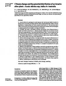
F I G U R E 1 (a) Track and intensity of Cyclone Yasi (BOM, 2011), (b) location of Hinchinbrook Island, and (c) average wind speed zones from Cyclone Yasi (NSPR, 2011)
|
3
ASBRIDGE et al.
north of Hinchinbrook Island (Figure 1a), which supports the largest
Within Australia, there has been increasing concern regarding
contiguous area of mangroves in Australia. The 500-km-diameter
the impacts of climate change on the long-term health of mangroves
cyclone (with an eye of 30 km) generated wind gusts up to 285 km/
and the impacts on biodiversity as well as society and economics.
hr, and maximum wind speeds were estimated at 215 km/hr (10 min
This issue has gained greater prominence following the recent die-
average). Average wind strength zones are shown in Figure 1c. The
back event (Duke et al., 2017), which affected over 10,000 ha of
resultant storm surge caused a temporary sea-level rise of 7 m
mangroves in northern Australia. This was linked to a reduction in
(Beeden et al., 2015), and 12 m offshore waves and 6 m near-shore
sea level in accordance with a strong El Niño Southern Oscillation
waves (Haigh et al., 2014). The cyclone crossed land during high tide,
on the viability of mangrove communities and compromise their abil-
turn interval at once in 70 years for the tropical region of northern
ity to support ecosystem services. For this reason, this study aimed
Queensland. Figure 1. a) Track and intensity of Cyclone Yasi (Bureau
to:
of Meteorology, 2011), b) location of Hinchinbrook Island, and c) average wind speed zones from Cyclone Yasi (NSPR, 2011).
1. Quantify the loss and degradation of mangroves surrounding
The cyclone inflicted considerable damage on the mangroves
Hinchinbrook Island during and following Tropical Cyclone Yasi
surrounding Hinchinbrook Island. The Queensland Government re-
through time-series comparison of very high-resolution aerial
ported that 17.2% of the precyclone extent was affected by the cy-
and RapidEye imagery and temporal sequences of space-borne
clone. Aerial surveys north of (but not including) mangroves around
optical and Japanese Aerospace Exploration Agency (JAXA)
Hinchinbrook Island in 2011 and 2013 were undertaken to visually assess (using approximately 500 photographs) the extent of damage to major vegetation communities and the extent of recovery. The study concluded that vast areas of mangrove had experienced
L-band Synthetic Aperture Radar (SAR) data. 2. Establish the extent to which mangroves had recovered from the cyclone. 3. Suggest a number of hypotheses to explain the patterns of man-
dieback with this potentially attributed to the inability of some
grove mortality and recovery and provide an insight into the long-
mangroves species to adapt to the variation in salinity associated
term recovery of mangroves.
with changes in sediment dynamics, hydrology, and a storm surge. Previous studies confirm that although many species are tolerant to
Short- and long-term impacts of cyclone activity and recovery tra-
changes in salinity, a number of species experience reduced photo-
jectories are discussed below with both global and local examples. The
synthesis and growth (Lin & Sternberg, 1993). One of the proposed
location, land use, climate, ocean circulation, tidal regime, and biodiver-
solutions for recovery at Hinchinbrook Island is to “let nature take its
sity of Hinchinbrook Island are presented, and the available data and
course” (Holloway, 2013).
methods of data analysis are described. The results present a time series of FPC and HH and HV backscatter for the designated land cover classes and provide maps of mangrove loss. The reasons for change in mangrove structure and health and the patterns of destruction and recovery are discussed with reference to global and future implications.
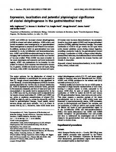
2 | BAC KG RO U N D Tropical storms (cyclones, typhoons and hurricanes) are common along the World’s tropical and subtropical coastlines and can exert considerable damage to mangroves, which may be wind and/ or water driven. The following sections provide an overview of the impacts of these storms over varying time frames and focus on mechanical damage, sediment erosion and accretion, inundation and salinity changes. An overview of the physical changes in the environF I G U R E 2 The water level measured at Cardwell tide gauge indicating a peak when Cyclone Yasi crossed the coastline (Queensland Government, 2015)
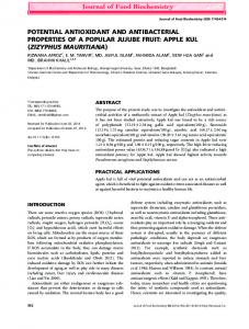
ment together with the positive and negative implications for mangroves forests is presented in Figure 3. Although this investigation does not directly measure the changes to sediment and hydrological
|
ASBRIDGE et al.
4
F I G U R E 3 The physical changes following cyclonic activity and the resultant positive (P) and negative (N) implications for mangroves dynamics, this figure provides a clear summary of the processes af-
complete burial of many pneumatophores resulted in mass mortal-
fected by direct and indirect cyclonic activity. It is important to un-
ity in the following year (Hopley, 1974). Similarly, following major
derstand the array of positive and negative implications, in order to
flooding in January 2011, 92% of the mangroves along 76 km of the
comprehend the complexity of the short- and long-term recovery
Brisbane River experienced mortality as a result of inundation and
trajectories.
erosion (Asbridge et al., 2015; Dowling, 2012). Following Hurricane Andrew in Florida in 1992, erosion of sediments (by an average of
2.1 | Mechanical damage
2–3 cm (Cahoon et al., 2003)) led to the uprooting of trees which further exposed previously protected land behind the forest to wind
In the short term, mangroves experience direct destruction from
and wave action (Doyle et al., 1995; Swiadek, 1997). Collapse of sed-
wind action, including windthrow, crown damage (defoliation and
iments can continue until affected areas are stabilized by roots from
snapping of small to large branches), bole damage, and mortality
newly established propagules or surviving mangroves.
(Kjerfve, 1990; Stocker, 1976). In the long term, changes in the distribution, species composition, and growth can occur as a consequence of changes in sediment dynamics (erosion, accretion) and hydrology
2.2.2 | Accretion
(inundation, drainage (Jimenez, Lugo, & Cintron, 1985)); these sec-
During and following large storms, substantive movement of eroded
ondary effects may only become apparent months after the storms
sediments is typical and where the subsequent deposition is exces-
and may persist for many years (Gilman et al., 2008; Smith, Robblee,
sive, mangroves may suffer because of the reduced ability to respire
Wanless, & Doyle, 1994).
from roots and oxygen deficit stress particularly where this is in excess of >10 cm/year above normal rates. The rate and extent of mortality
2.2 | Sediment redistribution 2.2.1 | Erosion
depend upon the degree of burial, with species with prop roots (e.g., Rhizophora and Bruguiera) being more tolerant compared to those with pneumatophores (e.g., Avicennia spp.; (Ellison, 1999; Paling, Kobryn, & Humphreys, 2008)). Once the roots have died, the sediment and
During the storm event, strong winds, currents, and waves can lead
decomposing roots can become anoxic, resulting in a decrease in
to significant erosion of the substrate material (Swiadek, 1997) and
the redox potential and an increase in the concentration of sulfides
undercutting of mangroves. As an example, significant erosion oc-
(Mendelssohn, Kleiss, & Wakeley, 1995). Without the supportive root
curred in Bowling Green Bay south of Townsville, north Queensland,
systems, sediment elevations may reduce through decomposition of
and along the eastern region of the Burdekin Delta following
organic matter but the amount will vary within the mangrove system.
Cyclone Althea in December 1971 when water overtopped ridges
For example, basin mangroves often experience sediment collapse
and banks, with many mangroves uprooted or sand-blasted by the
over a longer period of time compared to fringe mangroves because of
wind. Although the majority of mangroves were able to recover, the
differences in sediment structure and the different susceptibilities of
|
5
ASBRIDGE et al.
mangroves to dieback. Where the growth rates and densities of roots
(particularly fine) are high (as in the case of Rhizophora species that
et al., 2011; Morrisey et al., 2010). Saline tolerance varies among spe-
often dominate fringe mangroves) and rates of root decomposition
cies due to their morphological and physiological adaptations. In this
are low, sediment strengths tend to be greater (Cahoon et al., 2003;
way, the abrupt salinity change and continuous inundation may ren-
Middleton & Mckee, 2001). Hence, forests dominated by species such
der mangroves unable to make physiological adjustments, potentially
as Rhizophora may be less vulnerable to collapse and recovery may
resulting in reduced forest diversity, structure, and overall resilience.
be greater compared to other species occurring in other elevation zones. Sedimentation following cyclones can also alter flushing regimes, as a consequence of changes in topography. Areas of standing
2.5 | Recovery of mangroves
water may remain where sediment obstructs flows, with this further
Mangrove recovery is often facilitated by growth from reserve or
reducing oxygen concentration and redox potential (Bardsley, Davie,
secondary meristematic tissues, sprouting from trunks or branches,
& Woodroffe, 1985; Mendelssohn et al., 1995).
or establishment from propagules. Such growth is variable and depends on the extent and severity of damage, water flows during and
2.3 | Inundation
following the cyclone (removing or depositing propagules), and the species type (Imbert, Rousseau, & Labbe, 1998; Smith et al., 1994).
During the early phases of inundation, the influx of water can re-
Recovery also depends upon the rate of peat collapse which, when
move litter layers and propagules which reduces recruitment, pro-
combined with poor propagule production, prevents rapid coloniza-
ductivity, and in situ carbon cycling (Forbes & Cyrus, 1992). Where
tion and leads to sediment instability, reductions in elevation, and
inundation occurs for long periods of time, the health and produc-
subsequent tidal inundation, factors that all limit further propagule
tivity of mangroves can be affected. As examples, a cyclone struck
establishment (Lugo & Patterson-Zucca, 1977).
the Kosi Estuary in South Africa in January 1966, which resulted in a 6 m rise in water level and when Cyclone Domoina made landfall at Natal, South Africa, in January 1984, large areas of the two main
3 | S T U DY A R E A
river channels were eroded with the rivers retreating by 100 m and widening by 300 m in some locations, with the depth increasing by
Hinchinbrook Island is one of Australia’s largest national parks (39,350 ha),
10–14 m. The increased amount of water led to significant mortal-
located in the Coral Sea 8 km southeast of Cardwell, Queensland
ity of mangroves (Breen & Hill, 1969; Forbes & Cyrus, 1992) and,
(18.33°S, 146.22°E) (Figure 1b). The Island is only accessible via boat
in the latter case, the magnitude related directly to the period of
and is uninhabited with the exception of a small tourist resort at Cape
submersion and the height of mangroves. Many of the smallest sap-
Richards. The predominant land use is tourism, principally marine-based
lings (15 knots) travel over a comparatively short fetch, in a southeasterly direction cre-
2.4 | Salinity changes
ating short wind waves (rarely >1 m) and a southerly tidal flow (Pye & Rhodes, 1985). By contrast, large storm waves are produced in
Mangroves are halophytes, thriving in saline conditions whereby sa-
the wet season as a result of cyclonic activity (Belperio, 1978; Pye &
linity plays a significant role in regulating the growth and distribu-
Rhodes, 1985). The southeasterly trade winds generate a longshore
tion of the forests (Waisel, 1972). Inundation resulting from storm
current in a northerly direction along the inshore of the island.
surges and changed hydrological dynamics following cyclonic activ-
Hinchinbrook Island is one of the most biologically diverse and
ity is associated with increased salinity and saltwater intrusion. High
species-rich continental islands in the Great Barrier Reef with 54 eco-
salinity can limit growth rates, productivity, propagule production,
systems (Stanton & Godwin, 1989) (46 are declared as being of con-
fecundity, seedling survival, and decrease hydraulic conductivity,
cern or endangered, with the four remaining not found in any other
leaf water potential, stomatal conductance, and photosynthesis (Ball,
protected regions in Queensland; (Van Riper et al., 2012)). There are
|
ASBRIDGE et al.
6
vast and diverse mangrove stands, with 31 species identified that form
defined as the proportion of a pixel containing the vertical projec-
structurally diverse communities ranging from stunted/dwarf regions
tion of vegetation (Armston, Denham, Danaher, Scarth, & Moffiet,
to mature forests with canopy heights >40 m (Bunt, Williams, & Clay,
2009). FPC mapping only uses dry season (May to November) im-
1982; Ellison, 2000). Dominant species include Rhizophora apiculata,
agery in an automated classification at 25 m resolution. The FPC for
R. stylosa, Rhizophora lamarckli, Ceriops australis, Ceriops tagal, and
mature mangroves is usually > 80% because of the high density of
Bruguiera gymnorhiza (Boto & Bunt, 1981; Clough, 1998). The two
trees with a full canopy and a threshold of 30% FPC (equating to
largest regions of mangrove forest occur at Missionary Bay (approxi-
50% canopy cover) can consistently delineate the majority of man-
mately 20 km2) and within the Hinchinbrook Channel (approximately
groves from other vegetation and mudflats (Asbridge & Lucas, 2016).
164 km2), which together denote one of the largest neighboring mangrove forests in Australia (Clough, 1998). In 1997, the mangroves on Hinchinbrook Channel were, on average, >50 years old and approxi-
4.1.2 | ALOS
mately 10 m in height (Duke, 1997). From 1943 to 1991, there was no
Advanced Land Observing Satellite (ALOS) Phased Arrayed L-band
significant change in the total area of mangrove or saltmarsh at the
SAR (PALSAR) Fine Beam Single (FBS; HH polarization), Dual (FBD;
island in the Hinchinbrook Channel. However, there was a substantial
HH and HV polarization), and Polarimetric (PS; HH, VV, HV) data
net change in the proportions of intertidal vegetation, as 78% of the
were acquired over Hinchinbrook Island prior to and following
saltmarsh (and some small areas of short mangroves) were replaced
Cyclone Yasi by the Japanese Space Exploration Agency (JAXA).
by tall mangrove forests, with this change attributed to variations in
These were made available through the Japanese Space Exploration
rainfall (Ebert, 1995; cited in Duke, 1995). Mangroves also proliferate
Agency (JAXA’s) Kyoto and Carbon (K&C) Initiative. The ALOS-
in the sheltered sand dunes at Ramsay Bay on unconsolidated sedi-
PALSAR data were converted to Gamma0 using coefficients pro-
ments (colluvial and alluvial) and in between Deluge and Gayundah
vided by JAXA (Shimada, Isoguchi, Tadono, & Isono, 2009).
Inlets (Queensland Parks and Wildlife Service, 2016).
L-band microwaves penetrate through foliage and interact pre-
The distribution of mangroves on Hinchinbrook Island is partly
dominantly with the woody parts of the mangrove (i.e., the trunk
controlled by exposure, with the seaward (exposed) side of the is-
and branches). Waves that are transmitted horizontally and return to
land devoid of mangroves, except for a sheltered area behind a sand
the sensor in a vertical orientation (HV) indicate volume scattering
barrier. In contrast, the western side is protected and has extensive
within the branches of the canopy. Horizontally transmitted waves
forests (Galloway, 1982). In addition, tidal action also influences dis-
returning in a horizontal orientation (HH) have typically experienced
tribution via the dispersal and establishment of propagules. For in-
double-bounce interaction, between the trunks and the sediment.
stance, at the northern end of the island the mangroves extend 5 km
ALOS-PALSAR data are influenced by vegetation water content, in-
along the sheltered side of a tombolo and are distributed adjacent to
cluding that on that associated with rainfall (Lucas et al., 2010).
tidal channels. Within the sheltered Hinchinbrook Channel, the forests follow the complex network of tidal channels and exhibit explicit zonation (Galloway, 1982). The tidal dynamics surrounding the island
4.1.3 | Digital photography and RapidEye
are asymmetrical partly due to the mangroves forests (Wolanski,
RapidEye data acquired in 2014 were made available through the
Jones, & Bunt, 1980). At the southern end of the island, the flood
Planetlabs Ambassador Program. The recent acquisition of the data,
tidal current flows in a northerly direction, whereas at the northern
which has a resolution of 6.5 m provided an opportunity to map the
end of the island the current is southerly. This allows the tidal chan-
extent of damage to mangroves following Cyclone Yasi. However,
nel to remain open and deep through self-scouring (Galloway, 1982).
high tide prevented the sole use of RapidEye data for land cover clas-
The forests are predominantly influenced by saline water, with
sification, particularly as nonvegetated areas such as mudflats were
freshwater influxes only experienced during periods of intense/per-
not visible. The RapidEye data were therefore used in combination
sistent rainfall and/or low tide (Lear & Turner, 1977). However, the
with digital aerial photography provided by the Queensland Globe as
island within Hinchinbrook Channel is influenced by river discharge
open access data within Google Earth. The imagery was provided by
from both the mainland and runoff from Hinchinbrook Island.
the Department of Natural Resources and Mines.
4 | M E TH O DS
4.1.4 | Ancillary data
4.1 | Available data 4.1.1 | Landsat foliage projective cover
Daily rainfall data were obtained over the period of the ALOS- PALSAR acquisitions at Cardwell Range (146.18°E, 18.55°S) to establish whether variations in L-band SAR backscatter were attributed to changes in rainfall rather than actual vegetation cover. To define the
To determine changes in foliage cover following Cyclone Yasi, an an-
extent of mangroves prior to the cyclone, Regional Ecosystem maps
nual time series of Landsat-derived foliage projective cover (FPC)
were obtained via the Queensland Herbarium. In addition, a map of
from 1987 to 2016 was obtained from the Queensland Department
Hinchinbrook National Park was also acquired from the Department
of Science, Information Technology and Innovation (DSITI). FPC is
of National Parks, Sport and Racing.
|
7
ASBRIDGE et al.
4.2 | Data processing and analysis
Queensland coastline. An accuracy assessment was conducted using randomly sampled points for surviving and dead mangroves. The
The regional ecosystem map was used to define the wetland region
percentage change in the FPC prior to (2009) and following (2015)
surrounding Hinchinbrook Island, which included mangroves and
the cyclone was mapped using the following equation: ((FPC 2009
mudflats. This region was then classified into four broad land cover
- FPC 2015)/FPC 2009)*100. The regions of surviving and dead
classes (surviving mangroves, dead mangroves, other vegetation (i.e.,
mangroves, created from the maximum-likelihood classification,
rainforest), and nonvegetated mudflats) by applying a maximum-
were overlain onto the FPC change map to identify the presence or
likelihood classification to RapidEye (2015) data. Randomly sampled
absence of recovery.
points were located and allocated to the four land cover classes by referencing Landsat FPC (2009 and 2015) and Queensland Globe (2016) imagery. These were used to train the classifier and subsequently determine the accuracy of the classification. For each class, 120 regions of interest (ROIs; typically