The Fallacy of Placing Confidence in Confidence Intervals Richard D. Morey
Rink Hoekstra
Cardiff University
University of Groningen
Jeffrey N. Rouder
Michael D. Lee
University of Missouri
University of California-Irvine
Eric-Jan Wagenmakers University of Amsterdam Interval estimates – estimates of parameters that include an allowance for sampling uncertainty – have long been touted as a key component of statistical analyses. There are several kinds of interval estimates, but the most popular are confidence intervals (CIs): intervals that contain the true parameter value in some known proportion of repeated samples, on average. The width of confidence intervals is thought to index the precision of an estimate; CIs are thought to be a guide to which parameter values are plausible or reasonable; and the confidence coefficient of the interval (e.g., 95%) is thought to index the plausibility that the true parameter is included in the interval. We show in a number of examples that CIs do not necessarily have any of these properties, and can lead to unjustified or arbitrary inferences. For this reason, we caution against relying upon confidence interval theory to justify interval estimates, and suggest that other theories of interval estimation should be used instead.
“You keep using that word. I do not think it means what you think it means.” Inigo Montoya, The Princess Bride (1987)
The development of statistics over the past century has seen the proliferation of methods designed to allow inferences from data. Methods vary widely in their philosophical foundations, the questions they are supposed to address, and their frequency of use in practice. One popular and widely-promoted class of methods comprises interval estimates. There are a variety of approaches to interval estimation, differing in their philosophical foundation and computation, but informally all are supposed to be estimates of a parameter that account for measurement or sampling uncertainty by yielding a range of values for the parameter instead of a single value. Of the many kinds of interval estimates, the most popular is the confidence interval (CI). Confidence intervals are introduced in almost all introductory statistics texts; they are recommended or required by the methodological guidelines of
Address correspondence to Richard D. Morey (
[email protected]). We thank Mijke Rhemtulla for helpful discussion during the drafting of the manuscript. Supplementary material, all code, and the source for this document are available at https: //github.com/richarddmorey/ConfidenceIntervalsFallacy. Draft date: August 26, 2015.
many prominent journals (e.g., Psychonomics Society, 2012; Wilkinson & the Task Force on Statistical Inference, 1999); and they form the foundation of methodological reformers’ proposed programs (G. Cumming, 2014; Loftus, 1996). In the current atmosphere of methodological reform, a firm understanding of what sorts of inferences confidence interval theory does, and does not, allow is critical to decisions about how science is done in the future. In this paper, we argue that the advocacy of CIs is based on a folk understanding rather than a principled understanding of CI theory. We outline three fallacies underlying the folk theory of CIs, and place these in the philosophical and historical context of CI theory proper. Through an accessible example adapted from the statistical literature, we show how CI theory differs from the folk theory of CIs. Finally, we show the fallacies of confidence in the context of a CI advocated and commonly used for ANOVA and regression analysis, and discuss the implications of the mismatch between CI theory and the folk theory of CIs. Our main point is this: confidence intervals should not be used as modern proponents suggest because this usage is not justified by confidence interval theory. The benefits that modern proponents see CIs as having are considerations outside of confidence interval theory; hence, if used in the way CI proponents suggest, CIs can provide severely misleading inferences. For many CIs, proponents have not actually explored whether the CI supports reasonable inferences or not. For this reason, we believe that appeal to CI theory is re-
2
MOREY ET AL.
dundant in the best cases, when inferences can be justified outside CI theory, and unwise in the worst cases, when they cannot. The Folk Theory of Confidence Intervals In scientific practice, it is frequently desirable to estimate some quantity of interest, and to express uncertainty in this estimate. If our goal were to estimate the true mean µ of a normal population, we might choose the sample mean x¯ as an estimate. Informally, we expect x¯ to be close to µ, but how close depends on the sample size and the observed variability in the sample. To express uncertainty in the estimate, CIs are often used. If there is one thing that everyone who writes about confidence intervals agrees on, it is the basic definition: A confidence interval for a parameter — which we generically call θ and might represent a population mean, median, variance, probability, or any other unknown quantity — is an interval generated by a procedure that, on repeated sampling, has a fixed probability of containing the parameter. If the probability that the process generates an interval including θ is .5, it is a 50% CI; likewise, the probability is .95 for a 95% CI. Definition 1 (Confidence interval) An X% confidence interval for a parameter θ is an interval (L, U) generated by a procedure that in repeated sampling has an X% probability of containing the true value of θ, for all possible values of θ (Neyman, 1937).1 The confidence coefficient of a confidence interval derives from the procedure which generated it. It is therefore helpful to differentiate a procedure (CP) from a confidence interval: an X% confidence procedure is any procedure that generates intervals containing θ in X% of repeated samples, and a confidence interval is a specific interval generated by such a process. A confidence procedure is a random process; a confidence interval is observed and fixed. It seems clear how to interpret a confidence procedure: it is any procedure that generates intervals that will contain the true value in a fixed proportion of samples. However, when we compute a specific interval from the data and must interpret it, we are faced with difficulty. It is not obvious how to move from our knowledge of the properties of the confidence procedure to the interpretation of some observed confidence interval. Textbook authors and proponents of confidence intervals bridge the gap seamlessly by claiming that confidence intervals have three desirable properties: first, that the confidence coefficient can be read as a measure of the uncertainty one should have that the interval contains the parameter; second, that the CI width is a measure of estimation uncertainty; and third, that the interval contains the “likely” or “reasonable” values for the parameter. These all involve reasoning about
the parameter from the observed data: that is, they are “postdata” inferences. For instance, with respect to 95% confidence intervals, Masson and Loftus (2003) state that “in the absence of any other information, there is a 95% probability that the obtained confidence interval includes the population mean.” G. Cumming (2014) writes that “[w]e can be 95% confident that our interval includes [the parameter] and can think of the lower and upper limits as likely lower and upper bounds for [the parameter].” These interpretations of confidence intervals are not correct. We call the mistake these authors have made the “Fundamental Confidence Fallacy” (FCF) because it seems to flow naturally from the definition of the confidence interval: Fallacy 1 (The Fundamental Confidence Fallacy) If the probability that a random interval contains the true value is X%, then the plausibility or probability that a particular observed interval contains the true value is also X%; or, alternatively, we can have X% confidence that the observed interval contains the true value. The reasoning behind the Fundamental Confidence Fallacy seems plausible: on a given sample, we could get any one of the possible confidence intervals. If 95% of the possible confidence intervals contain the true value, without any other information it seems reasonable to say that we have 95% certainty that we obtained one of the confidence intervals that contain the true value. This interpretation is suggested by the name “confidence interval” itself: the word “confident”, in lay use, is closely related to concepts of plausibility and belief. The name “confidence interval” — rather than, for instance, the more accurate “coverage procedure” — encourages the Fundamental Confidence Fallacy. The key confusion underlying the FCF is the confusion of what is known before observing the data — that the CI, whatever it will be, has a fixed chance of containing the true value — with what is known after observing the data. Frequentist CI theory says nothing at all about the probability that a particular, observed confidence interval contains the true value; it is either 0 (if the interval does not contain the parameter) or 1 (if the interval does contain the true value). We offer several examples in this paper to show that what is known before computing an interval and what is known after computing it can be different. For now, we give a simple example, which we call the “trivial interval.” Consider the problem of estimating the mean of a continuous population with two independent observations, y1 and y2 . If y1 > y2 , we construct an confidence interval that contains all real numbers (−∞, ∞); otherwise, we construct an empty confidence 1
The modern definition of a confidence interval allows the probability to be at least X%, rather than exactly X%. This detail does not affect any of the points we will make; we mention it for completeness.
FUNDAMENTAL CONFIDENCE FALLACY
interval. The first interval is guaranteed to include the true value; the second is guaranteed not too. It is obvious that before observing the data, there is a 50% probability that any sampled interval will contain the true mean. After observing the data, however, we know definitively whether the interval contains the true value. Applying the pre-data probability of 50% to the post-data situation, where we know for certain whether the interval contains the true value, would represent a basic reasoning failure. Post-data assessments of probability have never been an advertised feature of CI theory. Neyman, for instance, said “Consider now the case when a sample...is already drawn and the [confidence interval] given...Can we say that in this particular case the probability of the true value of [the parameter] falling between [the limits] is equal to [X%]? The answer is obviously in the negative” (Neyman, 1937, p. 349). According to frequentist philosopher Mayo (1981) “[the misunderstanding] seems rooted in a (not uncommon) desire for [...] confidence intervals to provide something which they cannot legitimately provide; namely, a measure of the degree of probability, belief, or support that an unknown parameter value lies in a specific interval.” Recent work has shown that this misunderstanding is pervasive among researchers, who likely learned it from textbooks, instructors, and confidence interval proponents (Hoekstra, Morey, Rouder, & Wagenmakers, 2014). If confidence intervals cannot be used to assess the certainty with which a parameter is in a particular range, what can they be used for? Proponents of confidence intervals often claim that confidence intervals are useful for assessing the precision with which a parameter can be estimated. This is cited as one of the primary reasons confidence procedures should be used over null hypothesis significance tests (e.g., G. Cumming & S. Finch, 2005; G. Cumming, 2014; Fidler & Loftus, 2009; Loftus, 1993, 1996). For instance, G. Cumming (2014) writes that “[l]ong confidence intervals (CIs) will soon let us know if our experiment is weak and can give only imprecise estimates” (p. 10). Young and Lewis (1997) state that “[i]t is important to know how precisely the point estimate represents the true difference between the groups. The width of the CI gives us information on the precision of the point estimate” (p. 309). This is the second fallacy of confidence intervals, the “precision fallacy”: Fallacy 2 (The Precision fallacy) The width of a confidence interval indicates the precision of our knowledge about the parameter. Narrow confidence intervals show precise knowledge, while wide confidence errors show imprecise knowledge. There is no necessary connection between the precision of an estimate and the size of a confidence interval. One way to see this is to imagine two researchers — a senior researcher and a PhD student — are analyzing data of 50 participants
3
from an experiment. As an exercise for the PhD student’s benefit, the senior researcher decides to randomly divide the participants into two sets of 25 so that they can separately analyze half the data set. In a subsequent meeting, the two share with one another their Student’s t confidence intervals for the mean. The PhD student’s 95% CI is 52 ± 2, and the senior researcher’s 95% CI is 53 ± 4. The senior researcher notes that their results are broadly consistent, and that they could use the equally-weighted mean of their two respective point estimates, 52.5, as an overall estimate of the true mean. The PhD student, however, argues that their two means should not be evenly weighted: she notes that her CI is half as wide and argues that her estimate is more precise and should thus be weighted more heavily. Her advisor notes that this cannot be correct, because the estimate from unevenly weighting the two means would be different from the estimate from analyzing the complete data set, which must be 52.5. The PhD student’s mistake is assuming that CIs directly indicate post-data precision. Later, we will provide several examples where the width of a CI and the uncertainty with which a parameter is estimated are in one case inversely related, and in another not related at all. We cannot interpret observed confidence intervals as containing the true value with some probability; we also cannot interpret confidence intervals as indicating the precision of our estimate. There is a third common interpretation of confidence intervals: Loftus (1996), for instance, says that the CI gives an “indication of how seriously the observed pattern of means should be taken as a reflection of the underlying pattern of population means.” This logic is used when confidence intervals are used to test theory (Velicer et al., 2008) or to argue for the null (or practically null) hypothesis (Loftus, 1996). This is another fallacy of confidence interval that we call the “likelihood fallacy”. Fallacy 3 (The Likelihood fallacy) A confidence interval contains the likely values for the parameter. Values inside the confidence interval are more likely than those outside. This fallacy exists in several varieties, sometimes involving plausibility, credibility, or reasonableness of beliefs about the parameter. A confidence procedure may have a fixed average probability of including the true value, but whether on any given sample it includes the “reasonable” values is a different question. As we will show, confidence intervals — even “good” confidence intervals, from a CI-theory perspective — can exclude almost all reasonable values, and can be empty or infinitesimally narrow, excluding all possible values (Blaker & Spjøtvoll, 2000; Dufour, 1997; Steiger, 2004; Steiger & Fouladi, 1997; Stock & Wright, 2000). But Neyman (1941) writes, “it is not suggested that we can ‘conclude’ that [the interval contains θ], nor that we should ‘be-
4
MOREY ET AL.
lieve’ that [the interval contains θ]...[we] decide to behave as if we actually knew that the true value [is in the interval]. This is done as a result of our decision and has nothing to do with ‘reasoning’ or ‘conclusion’. The reasoning ended when the [confidence procedure was derived]. The above process [of using CIs] is also devoid of any ‘belief’ concerning the value [...] of [θ].” (Neyman, 1941, pp. 133-134) It may seem strange to the modern user of CIs, but Neyman is quite clear that CIs do not support any sort of reasonable belief about the parameter. Even from a frequentist testing perspective where one accepts and rejects specific parameter values, Mayo and Spanos (2006) note that just because a specific value is in an interval does not mean it is warranted to accept it; they call this the “fallacy of acceptance.” This fallacy is analogous to accepting the null hypothesis in a classical significance test merely because it has not been rejected. If confidence procedures do not allow an assessment of the probability that an interval contains the true value, if they do not yield measures of precision, and if they do not yield assessments of the likelihood or plausibility of parameter values, then what are they? The theory of confidence intervals In a classic paper, Neyman (1937) laid the formal foundation for confidence intervals. It is easy to describe the practical problem that Neyman saw CIs as solving. Suppose a researcher is interested in estimating a parameter θ. Neyman suggests that researchers perform the following three steps:
is the frequency with which false values of a parameter are excluded. Better intervals are shorter on average, excluding false values more often (Lehmann, 1959; Neyman, 1937, 1941; Welch, 1939). Consider a particular false value of the parameter, θ0 , θ. Different confidence procedures will include that false value at different rates. If some confidence procedure CP A excludes θ0 , on average, more often than some CP B, then CP A is better than CP B for that value. Sometimes we find that one CP excludes every false value at a rate greater some other CP; in this case, the first CP is uniformly more powerful than the second. There may even be a “best” CP: one that excludes every false θ0 value at a rate greater than any other possible CP. This is analogous to a most-powerful test. Although a best confidence procedure does not always exist, we can always compare one procedure to another to decide whether one is better in this way (Neyman, 1952). Confidence procedures are therefore closely related to hypothesis tests: confidence procedures control the rate of including the true value, and better confidence procedures have more power to exclude false values. Early skepticism Skepticism about the usefulness of confidence intervals arose as soon as Neyman first articulated the theory (Neyman, 1934).2 In the discussion of Neyman (1934), Bowley, pointing out what we call the fundamental confidence fallacy, expressed skepticism that the confidence interval answers the right question: “I am not at all sure that the ‘confidence’ is not a ‘confidence trick.’ Does it really lead us towards what we need – the chance that in the universe which we are sampling the proportion is within these certain limits? I think it does not. I think we are in the position of knowing that either an improbable event has occurred or the proportion in the population is within the limits. To balance these things we must make an estimate and form a judgment as to the likelihood of the proportion in the universe [that is, a prior probability] – the very thing that is supposed to be eliminated.” (discussion of Neyman, 1934, p. 609)
a. Perform an experiment, collecting the relevant data. b. Compute two numbers – the smaller of which we can call L, the greater U – forming an interval (L, U) according to a specified procedure. c. State that L < θ < U – that is, that θ is in the interval. This recommendation is justified by choosing an procedure for step (b) such that in the long run, the researcher’s claim in step (c) will be correct, on average, X% of the time. A confidence interval is any interval computed using such a procedure. We first focus on the meaning of the statement that θ is in the interval, in step (c). As we have seen, according to CI theory, what happens in step (c) is not a belief, a conclusion, or any sort of reasoning from the data. Furthermore, it is not associated with any level of uncertainty about whether θ is, actually, in the interval. It is merely a dichotomous statement that is meant to have a specified probability of being true in the long run. Frequentist evaluation of confidence procedures is based on what can be called the “power” of the procedures, which
In the same discussion, Fisher critiqued the theory for possibly leading to mutually contradictory inferences: “The [theory of confidence intervals] was a wide and very handsome one, but it had been erected at considerable expense, and it was perhaps as well to count the cost. The first item to which he [Fisher] would call attention was the loss of uniqueness in the result, and the consequent danger of apparently contradictory inferences.” (discussion of Neyman, 1934, p. 618; 2
Neyman first articulated the theory in another paper before his major theoretical paper in 1937.
5
FUNDAMENTAL CONFIDENCE FALLACY
see also Fisher, 1935). Though, as we will see, the critiques are accurate, in a broader sense they missed the mark. Like modern proponents of confidence intervals, the critics failed to understand that Neyman’s goal was different from theirs: Neyman had developed a behavioral theory designed to control error rates, not a theory for reasoning from data (Neyman, 1941). In spite of the critiques, confidence intervals have grown in popularity to be the most widely used interval estimators. Alternatives — such as Bayesian credible intervals and Fisher’s fiducial intervals — are not as commonly used. We suggest that this is largely because people do not understand the differences between confidence interval, Bayesian, and fiducial theories, and how the resulting intervals cannot be interpreted in the same way. In the next section, we will demonstrate the logic of confidence interval theory by building several confidence procedures and comparing them to one another. We will also show how the three fallacies affect inferences with these intervals. Example 1: The lost submarine In this section, we present an example taken from the confidence interval literature (J. O. Berger & Wolpert, 1988; Lehmann, 1959; Pratt, 1961; Welch, 1939) designed to bring into focus the how CI theory works. This example is intentionally simple; unlike many demonstrations of CIs, no simulations are needed, and almost all results can be derived by readers with some training in probability and geometry. We have also created interactive versions of our figures to aid readers in understanding the example; see the figure captions for details. A 10-meter-long research submersible with several people on board has lost contact with its surface support vessel. The submersible has a rescue hatch exactly halfway along its length, to which the support vessel will drop a rescue line. Because the rescuers only get one rescue attempt, it is crucial that when the line is dropped to the craft in the deep water that the line be as close as possible to this hatch. The researchers on the support vessel do not know where the submersible is, but they do know that it forms two distinctive bubbles. These bubbles could form anywhere along the craft’s length, independently, with equal probability, and float to the surface where they can be seen by the support vessel. The situation is shown in Figure 1A. The rescue hatch is the unknown location θ, and the bubbles can rise from anywhere with uniform probability between θ − 5 meters (the bow of the submersible) to θ + 5 meters (the stern of the submersible). The rescuers want to use these bubbles to infer where the hatch is located. We will denote the first and second bubble observed by y1 and y2 , respectively; for convenience, we will often use x1 and x2 to denote the bubbles ordered by location, with x1 always denoting the smaller lo-
cation of the two. Note that y¯ = x¯, because order is irrelevant when computing means, and that the distance between the two bubbles is |y1 − y2 | = x2 − x1 . We denote this difference as d. The rescuers first note that from observing two bubbles, it is easy to rule out all values except those within five meters of both bubbles because no bubble can occur further than 5 meters from the hatch. If the two bubble locations were y1 = 4 and y2 = 6, then the possible locations of the hatch are between 1 and 9, because only these locations are within 5 meters of both bubbles. This constraints are formally captured in the likelihood, which is the joint probability density of the observed data for all possible values of θ. In this case, because the observations are independent, p(y1 , y2 ; θ)
=
py (y1 ; θ) × py (y2 ; θ)
The density for each bubble py is uniform across the submersible’s 10 meter length, which means the joint density must be 1/10 × 1/10 = 1/100. If the lesser of y1 and y2 (which we denote x1 ) is greater than θ − 5, then obviously both y1 and y2 must be. This means that the density, written in terms of x1 and x2 is: ( 1/100, if x1 > θ − 5 and x2 < θ + 5, p(x1 , x2 ; θ) = (1) 0 otherwise. If we write Eq. (1) as a function of the unknown parameter θ for fixed, observed data, we get the likelihood, which indexes the information provided by the data about the parameter. In this case, it is positive only when a value θ is possible given the observed bubbles (see also Figures 1 and 5): ( 1, θ > x2 − 5 and θ ≤ x1 + 5, p(θ; x1 , x2 ) = 0 otherwise. We replaced 1/100 with 1 because the particular values of the likelihood do not matter, only their relative values. Writing the likelihood in terms of x¯ and the difference between the bubbles d = x2 − x1 , we get an interval: ( 1, x¯ − (5 − d/2) < θ ≤ x¯ + (5 − d/2), p(θ; x1 , x2 ) = (2) 0 otherwise. If the likelihood is positive, the value θ is possible; if it is 0, that value of θ is impossible. Expressing the likelihood as in Eq. (2) allows us to see see several important things. First, the likelihood is centered around a reasonable point estimate for θ, x¯. Second, the width of the likelihood 10 − d, which here is an index of the uncertainty of the estimate, is larger when the difference between the bubbles d is smaller. When the bubbles are close together, we get have little information about θ compared to when the bubbles are far apart. With the likelihood as the information in the data in mind, we can define our confidence procedures.
6
MOREY ET AL.
A
Bayes
B
UMP Nonpara. Samp. Dist. Likelihood Bubbles
θ − 10
θ−5
θ
θ+5
θ + 10
Location
θ − 10
θ−5
θ
θ+5
θ + 10
Location
Figure 1. Submersible rescue attempts. Note that likelihood and CIs are depicted from bottom to top in the order in which they are described in the text. See text for details. An interactive version of this figure is available at http: //learnbayes.org/redirects/CIshiny1.html. Five confidence procedures A group of four statisticians3 happen to be on board, and the rescuers decide to ask them for help improving their judgments using statistics. The four statisticians suggest four different 50% confidence procedures. We will outline the four confidence procedures; first, we describe a trivial procedure that no one would ever suggest. An applet allowing readers to sample from these confidence procedures is available at the link in the caption for Figure 1. 0. A trivial procedure. A trivial 50% confidence procedure can be constructed by using the ordering of the bubbles. If y1 > y2 , we construct an interval that contains the whole ocean, (−∞, ∞). If y2 > y1 , we construct an interval that contains only the single, exact point directly under the middle of the rescue boat. This procedure is obviously a 50% confidence procedure; exactly half of the time — when y1 > y2 — the rescue hatch will be within the interval. We describe this interval merely to show that by itself, a procedure including the true value X% of the time means nothing (see also Basu, 1981). We must obviously consider something more than the confidence property, which we discuss subsequently. We call this procedure the “trivial” procedure. 1. A procedure based on the sampling distribution of the mean. The first statistician suggests building a confidence procedure using the sampling distribution of the mean x¯. The sampling distribution of x¯ has a known triangular distribution with θ as the mean. With this sampling distribution,
there is a 50% √ probability that x¯ will differ from θ by less than 5 − 5/ 2, or about 1.46m. We can thus use x¯ − θ as a so-called “pivotal quantity” (Casella & R. L. Berger, 2002, see the supplement to this manuscript for more details) by noting that there is a 50% probability that θ is within this same distance of x¯ in repeated samples. This leads to the confidence procedure √ x¯ ± (5 − 5/ 2), which we call the “sampling distribution” procedure. This procedure also has the familiar form x¯ ± C × S E, where here the standard error (that is, the standard deviation of the estimate x¯) is known to be 2.04. 2. A nonparametric procedure. The second statistician notes that θ is both the mean and median bubble location. Olive (2008) and Rusu and Dobra (2008) suggest a confidence procedure for the median that in this case is simply the interval between the two observations: x¯ ± d/2. It is easy to see that this must be a 50% confidence procedure; the probability that both observations fall below θ is .5 × .5 = .25, and likewise for both falling above. There is thus a 50% chance that the two observations encompass θ. Coincidentally, this is the same as the 50% Student’s t procedure for n = 2. We call this the “nonparametric” procedure. 3
John Tukey has said that the collective noun for a group of statisticians is “quarrel” (McGrayne, 2011).
FUNDAMENTAL CONFIDENCE FALLACY
3. The uniformly most-powerful procedure. The third statistician, citing Welch (1939), describes a procedure that can be thought of as a slight modification of the nonparametric procedure. Suppose we obtain a particular confidence interval using the nonparametric procedure. If the nonparametric interval is more than 5 meters wide, then it must contain the hatch, because the only possible values are less than 5 meters from both bubbles. Moreover, in this case the interval will contain impossible values, because it will be wider than the likelihood. We can exclude these impossible values by truncating the interval to the likelihood whenever the width of the interval is greater than 5 meters: ( x¯ ±
d 2
5−
d 2
if if
d