The Forecasting Error Statistics for convective-scale prediction: the impact of correlated errors in radar observations
13A.3
Kao-Shen Chung 1*, Isztar Zawadzki 1 , Luc Fillion 2 and Marc Berenguer 1 1 Department of Atmospheric and Oceanic Sciences, McGill University 2 Meteorological Research Branch, Environment Canada
1. Introduction Errors in forecasts, frequently referred to as background errors, result from the initial condition errors and errors growing from numerical algorithms as sources of forecast uncertainty. Estimating the forecast error is not straightforward since the true atmospheric state is never exactly known. Ensemble forecasting is a feasible way to characterize the forecasting errors and represent the probability of atmospheric states. In this latter context, radar observation error specifications have mostly neglected spatially correlated observation errors. As a counter-example, it is demonstrated here, using one realistic case, in the framework of the McGill data assimilation system (Chung et al. 2009), that this approximation needs to be revisited. The main objective is to demonstrate the impact of correlated perturbations (that simulate the observation errors) on the ensemble statistics, and also explore in more details the flow-dependent forecasting errors at convective scale.
2. Description of the assimilation system and MC2 model 2.1 Assimilation system The McGill data assimilation system for very short-term forecasting at convective scales (Laroche and Zawadzki 1994, Caya 2001) is used in this study. It is based on the variational formalism with a cost function including a background term, observations and cloud-resolving model equations as weak constraints. The system assimilates both radar reflectivity and Doppler velocity observations. Chung et. al (2009) presented the recent upgrades to the McGill assimilation system: 1) a preconditioning procedure is done in the assimilation system to avoid inverting the background error covariance, B −1 ; 2) assuming that the error covariance of the control variables is isotropic and * Corresponding author address: Kao-Shen Chung, Atmospheric and Oceanic Sciences, McGill University, 805 Sherbrooke W., Montreal, QC. H3A 2K6, Canada; E-mail:
[email protected]
homogeneous, the background error covariance matrix is modeled by a recursive filter, following Purser et al. (2003); 3) a prior high resolution (1km) model forecast is used as background field. With one assimilation cycle, the analysis fields from the assimilation system successfully trigger the convective storms in the radar observed regions. 2.2 Cloud-resolving model The Canadian Mesoscale Compressible Community (MC2) model (Laprise et al., 1997) is used as the cloud model in the current study. The algorithm is semi-Lagrangian in advection with semi-implicit in time step. A complete warm and cold microphysical parameterizations (Kong and Yau 1997) are included in the model. The model uses a one-way (cascade) nesting strategy, where a coarse-grid forecast provides initial and boundary conditions for a fine-grid (1km) forecast, and there is no upscale feedback.
3. Design of the experiments Following Houtekamer et al. (1996), we have added simulated errors to the observations, and used the McGill data assimilation system to obtain a set of analyses in this case study. In most studies using radar data (Snyder and Zhang 2003, Tong and Xue 2005 and Xue et al. 2006), only the variance of the observation errors with zero mean is prescribed and perturbations with a Gaussian distribution are generated. To investigate the impact of the correlated structure of the observation errors (in space) on the ensemble forecasts, two types of perturbations are generated and taken as the observation errors: uncorrelated, known as white noise (hereafter, UNCP) and errors with prescribed correlations (hereafter, CORP). For the UNCP experiment, we have added 3D fields of uncorrelated, unbiased, Gaussian perturbations to 3D radar observations of reflectivity, Z, and Doppler velocity, Vr. In our case, we have respectively used σZ=2.5 dB -1 and σv=1ms . An example of uncorrelated perturbations for reflectivity in the horizontal and the corresponding power spectrum are shown in Fig. 1.
For the CORP experiment, the error variances are the same as UNCP, and we have imposed a horizontal decorrelation distance of 10 km and a correlation of 0.85 at 250 m in the vertical for the reflectivity perturbations. The perturbations of Doppler velocity observations have been created with 5 km horizontal decorrelation distance, and 0.75 between contiguous layers. Fig. 2 illustrates the correlated perturbations in the horizontal and its corresponding power spectrum. Finally, to also consider the uncertainty in the background fields, in the third experiment, we perturb both observations (same way as CORP) and background fields at the initial time, (hereafter, CROB). We have chosen to perturb our background by using model forecasts for different lead times. By doing that we attempt to describe background errors as timing errors in the model fields. Prior high-resolution (1-km) MC2 simulations (without assimilating radar observations) at 1500 UTC, 1600 UTC and 1700 UTC are used as background fields in the ensemble forecasts. A case study is selected on 12 July 2004. It is a strong, long-lasting convective scale storm, and observed by the McGill S-band radar. Fig. 3 depicts the reflectivity observations of the storm at 1840 UTC and 1910 UTC.
(a)
(b)
(a)
Fig. 2. The same data set as in Fig. 1, but correlated observation error distribution in (a) space domain; (b) spectral domain.
(a) (b)
Fig. 1. (a) Realization of the normalized perturbation added to the Z fields; (b) Its corresponding averaged power spectrum.
(b)
σˆ X2 (z ) =
1 ( N − 1) × n x × n y
μˆ x (z ) =
and
nx
N nxn y
∑ ∑ [X (x, y, z ) − μˆ (z )] k =1 i , j =1
2
k
X
(4)
N nx n y
1 , X k ( x, y , z ) N × nx × n y k =1i , j =1
∑∑
(5)
and n y are the number of grid points in x and
y directions, and μˆ X (z ) is the estimated 2D mean value at z.
Fig. 3. Reflectivity observations of the McGill S-band radar on 12th July 2004 at (a)1840 UTC; (b) 1910 UTC. The dashed line indicates the analysis domain.
4. Results of the ensemble forecasting errors The ensemble forecasts were run over a one-hour period, from 12 July 2004 at 1810 UTC to 1910 UTC with a 1-km resolution. The ensemble forecasting error statistics are estimated by calculating the difference between each ensemble member and the ensemble mean as defined by:
B = (xb − x t )(xb − x t )T = εbεbT ≅< (xi − x )(xi − x )T > (1) where
xi
stands for each ensemble member and
x
is the ensemble mean valid at the same forecasting time. < > is the average of the members. The ensemble mean is over 10 realizations in the experiment of UNCP and CORP, and 30 members in the CROB. All the following results were computed within a domain of 140 x 70 km2 around the storm (see the dashed domain in Fig. 3). A perfect–model framework has been used for the ensemble experiments in order to simplify the interpretation of the results.
Figure 4 illustrates the spread in the 1-hour forecasts of horizontal wind u and vertical velocity obtained for the experiment UNCP. Both fields show significant spread around the convective storm. Since only observations were perturbed for this experiment and they are only available in precipitating areas, far away from the storm the spread is much smaller. Fig. 5 displays the spread of the forecast error as in Fig. 4 but for the CORP experiment. Both fields manifest larger spread around the storm as UNCP. However, one should notice that the significant difference between the two experiments is that in each grid point, the CORP experiment presents much larger spread for the variables in the analysis domain, and it is more evident near the location of the convective storm. The results of ensemble spread in UNCP and CORP indicate that by using the uncorrelated perturbations as observation errors, the error variance may be underestimated.
(a)
4.1 Ensemble Spread The ensemble spread at (x,y,z) for the control variable X has been computed as: N ⎫1 2 ⎧⎪ 2 ⎪ , (2) 1 S X (x, y,z) = ⎨ X x, y,z − X x, y,z ∑ k ( ) ( ) ⎬⎪ ⎪⎩ N −1 k=1 ⎭
[
]
N
1 where, is the ensemble mean X (x, y , z ) = X k (x, y , z ) N k =1
∑
at (x,y,z) with N-member realizations. Results are
(
)
expressed in terms of the S X x, y,z relative to the standard-deviation of the field of X at a height z,
σˆ X (z ) .
The Normalized Ensemble Spread is defined
as,
NES X ( x, y, z ) = where
S X ( x, y , z ) , σˆ X (z )
(3)
(b)
Fig. 4. Ensemble spread of 60-min forecast in UNCP at an altitude of 2.5km. (a) u component of the wind; (b) vertical velocity.
(b)
(a)
Fig. 6. Ensemble spread with 30 members of 60-min forecast from the experiment CROB. (a) u component of the horizontal wind; (b) vertical velocity. 4.2 Forecast Error correlations (b)
Here we investigate the impact of the forecasting error correlation in space. The error auto-correlation function (ACF),
ρˆ X , z , in the horizontal at a height z is
estimated as: N nx − L ny − M
ρˆ X , z ( L, M ) =
∑ ∑ ∑ ε ( x, y , z ) × ε ( x + L, y + M , z ) k =1 i =1
j =1
X ,k N
X ,k
nx
∑∑∑ ε (x, y, z ) k =1 i =1 j =1
Fig. 5. Ensemble spread of 60-min forecast in CORP at an altitude of 2.5km. (a) u component of the wind; (b) vertical velocity. Figure 6 is the ensemble spread resulting from a 30-members CROB experiment. The high uncertainty of the control variables (larger spread) is mainly distributed around the convective storm. However, as compared with results in experiment UNCP (Fig. 4.) and CORP (Fig. 5.), the ensemble spread is noticeable almost all over the entire analysis domain, and this could be due to the use of three different backgrounds. (a)
(6)
ny
2 X ,k
where is the ε X,k (x, y,z) = X k (x, y,z) − X (x, y,z) departure of the k-th member from the ensemble mean. L and M are the horizontal shift in the x and y directions, respectively. In the current study, the results are presented in the x direction. Error cross-correlations are also briefly described at the end of this subsection. Figure 7 presents the error ACF in the x direction computed from 5 individual members of the UNCP experiment for the wind components and temperature. One can see that the errors of u component have larger correlation in space than the vertical velocity errors. The error ACF resulting from the CORP experiment is shown in Fig. 8. The vertical velocity still decorrelates significantly in space as the UNCP experiment. However, one can notice that the errors in the horizontal wind in the CORP experiment are significantly more correlated in space than in the UNCP experiment. Similar results can be found in the v component and temperature as in the u component (results not shown). The comparison of error correlation in space between UNCP and CORP reveals that the error correlation decorrelates faster in space (except vertical velocity) when using uncorrelated perturbations as observation error. The error ACF in space for u component of the wind field at different heights in the experiment CROB is shown in Fig. 9a. The correlation is much longer compared to the experiments of UNCP and CORP. This larger error correlation in space is influenced by the use of three different backgrounds containing information from large (synoptic) scales. Figure 9-b shows the error ACF only within the precipitation area. It is manifest that the error decorrelates much faster as compared to the
result from the entire domain. This indicates the need to discriminate background error covariances within and outside the precipitating areas.
(b)
(a)
(b)
Fig. 8. ACF of the forecast error: 60-min forecast in x direction at an altitude of 2.5km for 5 realizations of the experiment CORP. (a) u component of the wind; (b) vertical velocity. (a)
Fig. 7. ACF of the forecast error: 60-min forecast in x direction at an altitude of 2.5km for 5 realizations of the experiment UNCP. (a) u component of the wind; (b) vertical velocity.
(b)
(a)
Fig. 9. ACF of the forecast error in u component of the wind for a lead time of 60-min forecast in x direction at different height of the experiment CROB: (a) computed in the entire analysis domain; (b) computed only within the precipitation region. Figure 10 depicts the cross-correlation errors between vertical velocity and cloud water mixing ratio at
each point within the convective cell (defined as the area in which the absolute value of vertical velocity is greater than 1ms-1). It is found in general that vertical velocity and cloud water mixing ratio show significant correlations with a horizontal correlation scale that significantly varies in the vertical. Similar results are found between vertical velocity and rain water cross-correlations. Those results illustrate the strong connection of the uncertainty between dynamics and microphysics processes.
Fig. 10. Cross-correlation errors between vertical velocity and cloud water within precipitation areas at 30-min forecast ( in x direction ).
5. Summary The current study showed how sensitive forecasting errors are to the representation of the observation error correlation. Based on this case study, our work is an attempt to add perturbations that account for the main sources of uncertainty in the initial conditions within a data assimilation system. The results show that the correlation of the errors greatly increases the spread of the ensemble as well as its correlation in space. In addition, the error correlation demonstrates the different characteristics within and outside precipitation areas, and cross-correlation errors reveal the strong coupling between dynamics and microphysics. Based on these findings, it appears desirable to account for those important components of error characterization within currently existing convective scale data assimilation schemes.
References Caya, A., 2001: Assimilation of radar observations into a cloud-resolving model, McGill University, 153 pp. Chung, K. S., I. Zawadzki, M. K. Yau, and L. Fillion, 2009: Short-term forecasting of a midlatitude convective storm by the assimilation of single Doppler radar observations. Monthly Weather Review.DOI: 10.1175/2009MWR2731.1 Houtekamer, P. L., L. Lefaivre, J. Derome, H. Ritchie, and H. L. Mitchell, 1996: A system simulation approach to ensemble prediction. Monthly Weather Review, 124, 1225-1242.
Kong, F., and M. K. Yau, 1997: An explicit approach to microphysics in MC2. Atmos.-Ocean, 35, 257-291. Laprise, R., D. Caya, G. Bergeron, and M. Giguere, 2 1997: The formulation of the Andre´ Robert MC (Mesoscale Compressible Community) Model. Atmos.–Ocean, 35, 195-220. Laroche, S. and I. Zawadzki, 1994: A Variational Analysis Method for Retrieval of 3-Dimensional Wind-Field from Single Doppler Radar Data. Journal of the Atmospheric Sciences, 51, 2664-2682. Purser, R. J., W.-S. Wu, D. F. Parrish, and N. M. Roberts, 2003: Numerical aspects of the application of recursive filters to variational statistical analysis. Part I: Spatially homogeneous and isotropic Gaussian covariances. Mon. Wea. Rev., 131, 1524-1535. Snyder, C. and F. Q. Zhang, 2003: Assimilation of simulated Doppler radar observations with an ensemble Kalman filter. Monthly Weather Review, 131, 1663-1677. Tong, M. J. and M. Xue, 2005: Ensemble Kalman filter assimilation of Doppler radar data with a compressible nonhydrostatic model: OSS experiments. Monthly Weather Review, 133, 1789-1807. Xue, M., M. J. Tong, and K. K. Droegemeier, 2006: An OSSE framework based on the ensemble square root Kalman filter for evaluating the impact of data from radar networks on thunderstorm analysis and forecasting. Journal of Atmospheric and Oceanic Technology, 23, 46-66.