The Form of Waiting Time Distributions of Continuous Time Random
Recommend Documents
May 12, 2008 - valenko in their theory of âthinningâ a renewal process. Turning our attention ..... The name continuous time random walk (CTRW) became popular in physics .... integral equation of the CTRW in the Laplace-Fourier domain as.
Nov 23, 2017 - tion waiting time Ïr. (i) whose probability density function. (PDF) Ïr i depends in ..... [13] C. I. Steefel, D. J. DePaolo, and P. C. Lichtner, Earth.
May 8, 2013 - arXiv:1305.1721v1 [cond-mat.stat-mech] 8 May 2013 ... may appear ergodic while the naked continuous time random walk exhibits weak ...
Jan 1, 2013 - 13 T. Sippel, J. Holdsworth, T. Dennis and J. Montgomery, PLOS ONE 6, ... 14 W. Min, L. Jiang, J. Yu, S.C. Kou, H. Qian and X.S. Xie, Nano Lett.
Dec 24, 2004 - a sequence of Bernoulli trials (m = 2), the success run of size k,. = S...S, is a simple pattern of size k. Let 1 and 2 be two simple patterns of ...
Aug 22, 2013 - arXiv:1304.4301v2 [cond-mat.mes-hall] 22 Aug 2013. Waiting Time Distributions for the Transport through a Quantum Dot Tunnel. Coupled to ...
Feb 13, 2018 - RB random walk [3] on G, as it will be needed in the continuous-time construction that follows. Once again we begin with a strongly connected ...
Apr 3, 2015 - exerts the irreversible electroporation [58] due to the external TTF ... A key quantity of this cancer treatment is localization of the electroporation.
Jun 6, 2018 - Abstract. We consider a continuous-time random walk which is defined as an interpolation of a random walk on a point process on the real line.
to describe the frequency at which the processors in the network fail, cf. [10]. In. âTechnische ..... on describe the mean time between failures. (MTBF) and let Ïe.
(2001). [31] V.V. Uchaikin, J. Exper. Theor. Phys. 97, 810 (2003). [32] V.E. Bening, V.Yu. Korolev, S. Koksharov, V.N. Kolokoltsov, J. Math. Sci. 146, 5950 (2007).
For fixed time re(t, ·) is a random variable which takes values in. {0, 1}, and for a fixed random sample re(·,Ï) is a realisation or scenario of the state process ...
converges to a reflected Brownian motion and the observation process converges ... of reflected Brownian motion, and for the filter of the rescaled queue model.
Waiting time guarantees improve customer satisfaction but be sure to meet ...... Following the training session, we asked the participants to imagine that they ...
Consider a random walk on the lattice of integers h with transition probabilities p,, (k + k + 1) and or = 1 -pI (k+ k - 1). Let T,,,, denote the first passage time from ...
Imagine two patients that wait the same amount of time to receive primary ... individual's satisfaction with waiting times (level of disutility) in a primary non-.
mother's brain surgery, he died in her lap on our way to Walgreens. Mr. Wilson loved car rides, and my mother loved including him. The time we spent waiting.
Waiting time guarantees improve customer satisfaction but be sure to meet them. ... Customers often have to wait during the process of acquiring and consuming ...
Waiting time distributions: unstratified. 01. 23. 100. 101. 102 ... Distribution of the waiting time (days) for state change 0 â 1 (acquire carriership) and 1 â 0 (lose ...
Nov 1, 2007 - by a number of authors (see [6, 10, 11] and the references in [2, 12]). ... the sequence is constrained up to time n, or the distribution of Yr given ...
ki[n]p(t â (i â 1)Ts â nTc) is the signature waveform for ..... random vector with probability density function (pdf). fzJ (¯z) = â ..... 4129â4140, 2009. [12] Y. H. Yun ...
Mar 15, 2013 - arXiv:1210.5618v2 [cond-mat.stat-mech] 15 Mar 2013. Ergodic properties of continuous-time random walks: finite-size effects and ensemble.
The Form of Waiting Time Distributions of Continuous Time Random
Dec 12, 2017 - School of Earth Sciences and Engineering, Nanjing University, Nanjing, ... distributions of waiting time in different dead-end pores show similar ...
Hindawi Geofluids Volume 2018, Article ID 8329406, 6 pages https://doi.org/10.1155/2018/8329406
Research Article The Form of Waiting Time Distributions of Continuous Time Random Walk in Dead-End Pores Yusong Hou, Jianguo Jiang
1. Introduction Anomalous dispersion widely exists in solute transport in ground water or in other porous media [1–7], which makes it difficult to simulate solute transport by traditional advectiondispersion equation. In recent years, scholars have developed a few models to describe the anomalous transport such as continuous time random walk (CTRW) [8–12] and fractional advection-dispersion equation [13–16]. The simulations by CTRW can agree well with the experimental data by fitting the transfer probability density function 𝜑(𝑥, 𝑡) [2, 17]. Assume 𝜑(𝑥, 𝑡) has the form 𝜑(𝑥, 𝑡) = 𝜙(𝑥)𝜓(𝑡), where 𝜓(𝑡) denotes the waiting time distribution between two successive jumps. Corresponding to anomalous transport, 𝜓(𝑡) should follow a power-law decline, that is, 𝜓(𝑡) ∼ 𝑡−1−𝛼 with 0 < 𝛼 < 2 [17]. Many researchers have investigated the form of 𝜓(𝑡) by simulating the transport of solute in porous media [18–21], which may show power-law decline. However, fitting parameters from transport data in complex fluid fields are not suitable to uncover the physical mechanism of the power-law decline. An alternative way for the investigation of the form of 𝜓(𝑡) is to directly simulate the motion of solute particles in immobile zones. In this paper, we construct the deadend pores as immobile zones and simulate the waiting time distributions to explore the modes of solute transport.
𝜓(𝑡) is more likely to show an exponential decline than a power-law decline because particles in stagnant zones are determined by diffusion equation. As many experiments show, an anomalous transport eventually converts to a Fickian process [2, 19]. Consequently, in the mathematical models, the power-law decline is often truncated arbitrarily by an exponential decline in the assumption of 𝜓(𝑡) [4, 9]. However, why does there exist a power-law decline of waiting time distribution? When does a power-law decline begin to convert to an exponential decline? In addition, it is not clear which factors determine the value of the power index 𝛼. To explore the general form of waiting time distribution function, we directly simulate 𝜓(𝑡) in dead-end pores. In this paper, we select three types of dead-end pores. By these deadend pores with different sizes and shapes, we aim to get a universal form of 𝜓(𝑡), which may show both the power-law part (corresponding to anomalous transport) and the exponential decline part (Fickian transport). In addition, from our simulations, we expect to get the index 𝛼 which describes the anomalous degree.
2. Method of Simulation In the framework of CTRW model for solute transport, the distribution of waiting time between two successive jumps
2
Geofluids Immobile zone bent tube Immobile zone straight tube
Solute molecules
Immobile zone hemisphere
Water flow Mobile zone
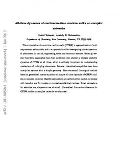
Figure 1: The schematic diagram of mobile zone and immobile zone. Three types of dead-end pores, that is, straight tube, bent tube, and hemisphere, represent the immobile zones.
determines whether the dispersion is anomalous or not. For simplicity, skipping over the displacement distribution 𝜙(𝑥) of jumps, we only investigate the waiting time distribution 𝜓(𝑡). In our physical picture, waiting events happen when nonreactive particles are trapped in immobile zones. Deadend pores are typical immobile zones. The flow velocity in a dead-end pore is zero and solute particles escape only by diffusion. The waiting time is the period from entering a dead-end pore to moving out of it. We consider three types of dead-end pores: straight tube, bent tube, and hemisphere as illustrated in Figure 1. These three dead-end pores lie above the flow tube which represents the mobile zone. Tracer particles on the interface between the flow tube and deadend pores may enter the dead-end pore by diffusion. We begin to count waiting time when the particles pass through interfaces to dead-end pores and end counting when particles pass through interfaces to the flow tube. For simplicity, we use the surviving probability 𝑃(𝑡) in the immobile zone to describe the waiting time distribution 𝜓(𝑡); the relation between them can be written as 𝑡
∞
0
𝑡
𝑃 (𝑡) = 1 − ∫ 𝜓 (𝜏) 𝑑𝜏 = ∫ 𝜓 (𝜏) 𝑑𝜏,
developed to simulate the random walk with variable weight [22–24]. We use the pruned-enriched method to adjust the weight according to 𝑃(𝑡). At the beginning of simulation, each particle is released at the interface between the flow tube and dead-end pores with the same weight 𝑊(0) = 1. Consider the case that the simulated particle is still in the dead-end pore at the time 𝑡 = 𝑛Δ𝑡. Define 𝑟 = 𝑊(𝑡)/𝑃(𝑡). If 𝑟 > 1, this particle is split in Int(𝑟) (the integer part of 𝑟) copies and each copy continues to diffuse with a new weight 𝑊new = 𝑊(𝑡)/Int(𝑟). If 𝑟 ≤ 1, we continue to simulate the diffusion of the particle with probability 𝑟 = 1/Int(1/𝑟) and the new weight 𝑊new is adjusted to 𝑊(𝑡)/𝑟 . In other words, the simulation of the particle is ceased with the probability 1 − 𝑟 . 𝑃(𝑡) is updated in every step. By the scheme of variable weight, the smallest probability we could simulate can be reduced by many orders of magnitude. In the whole range of simulated time, the number of samples for each 𝑡 has a nearly uniform distribution. Without the scheme of variable weights, the number of visited samples is proportional to 𝑃(𝑡) and decreases sharply with 𝑡, which leads to violent oscillation of simulated 𝑃(𝑡).
(1)
or Ψ(𝑡) = −𝑑𝑃(𝑡)/𝑑𝑡. Compared to 𝑃(𝑡), Ψ(𝑡) fluctuates more violently as the derivative enlarges the fluctuations of simulated values of 𝑃(𝑡). 𝑃(𝑡) can be directly calculated by counting the number of particles in the dead-end pores and the particles will not be tracked when they move out of immobile zones. Then, 𝜓(𝑡) is obtained from the derivative of 𝑃(𝑡). However, the probability 𝑃(𝑡) is very small when the time is large, especially if 𝑃(𝑡) decreases in an exponential form. By conventional particle tracing method with each particle of the same weight, 𝑃(𝑡) is proportional to the number of particles staying in the immobile zone. The number corresponding to small 𝑃(𝑡) is zero or fluctuates violently. To simulate 𝑃(𝑡) in a wide range, variable weight for tracing particles is adopted in this paper. In recent years the pruned-enriched method has been
3. Results and Discussion For most heavy metal ions, the order of magnitude of diffusion coefficient is about 10−10 m2 /s. In this paper, the diffusion coefficient of solute is set to be 4 × 10⁻¹⁰ m2 /s. When tracer particles enter the dead-end pores through the interface, we start the time. When particles escape from the dead-end pores, the tracing process of this particle will be terminated. For simplicity, particles after escaping from a dead-end pore cannot be allowed to enter the same deadend pore again because they drift in the flow tube (mobile zone). Firstly, we consider the surviving probability 𝑃(𝑡) in large dead-end pores. The lengths of straight tube and bent tube are both taken 10 mm and the radius of hemisphere is taken 15 mm. Figure 2 shows the power-law decrease of simulated 𝑃(𝑡) and 𝜓(𝑡). The 𝑃(𝑡) and 𝜓(𝑡) in bent tube and in
Geofluids
3 10−2
10−1 10−4
P 10−2
10−6
P ∼ t−
10−3
101
102
103
104
10−8
∼ t−1−
101
102
103
104
t (S)
t (S) = 0.51 straight tube = 0.51 bent tube = 0.52 hemisphere
Figure 2: The power-law form of the surviving probability 𝑃(𝑡) and the waiting time distribution Ψ(𝑡) in dead-end pores at early time. The power 𝛼 approximates to 0.5 for each type of dead-end pore.
hemisphere are reduced by the factor 1/2 and 1/4, respectively, which makes the comparison in Figure 2 clear without altering the power law. We take the values of power from the data of 𝑃(𝑡) because 𝜓(𝑡) has more violent fluctuations. During the time interval 10 s–104 s, 𝑃(𝑡) decays in a power law, that is, 𝑃(𝑡) ∼ 𝑡−𝛼 . Corresponding to straight tube, bent tube, and hemisphere, the value of 𝛼 is 0.50, 0.49, and 0.52, respectively. They are close to 0.5. Thus, it is reasonable to suppose that the power 𝛼 is approximately equal to 0.5 in these three types of dead-end pores. Let us discuss the physical meaning of the simulated results. This power-law form of 𝑃(𝑡) with 𝛼 = 0.5 results in anomalous dispersion, which can also be described by time-fractional advection-dispersion equation (tFADE). If the waiting time distribution has the form 𝜓(𝑡) ∼ 𝑡−1−𝛼 , the concentration 𝐶(𝑥, 𝑡) can be written as [25] 𝜕𝐶 (𝑥, 𝑡) = 0 𝐷𝑡1−𝛼 𝐿 [𝐶 (𝑥, 𝑡)] , 𝜕𝑡
(2)
where 0 𝐷𝑡1−𝛼 is the fractional Riemann-Liouville operator; that is, 1−𝛼 0 𝐷𝑡
𝑓 (𝜏) 1 𝜕 𝑡 𝑓 (𝑡) = . ∫ 𝑑𝜏 Γ (𝛼) 𝜕𝑡 0 (𝑡 − 𝜏)1−𝛼
(3)
Here, 𝐿[𝐶(𝑥, 𝑡)] is the operator representing dispersion. Therefore, the fractional order of time derivation is about 0.5 if anomalous dispersion is caused by solute trapping in long dead-end pores. The sizes of above dead-end pores are set large in the simulations. Let us consider the dead-end pores with short length. Tracer particles can jump out of them easily. Which form does surviving probability density 𝑃(𝑡) show? To investigate it, we set the length of straight tubes to be 1 mm, 2 mm, 3 mm, and 4 mm, respectively. The diffusion coefficient is the
same as above. The simulated 𝑃(𝑡) and 𝜓(𝑡) are illustrated in Figure 3. At the early time, 𝑃(𝑡) and 𝜓(𝑡) in each straight tube decrease with the power law. As time increases, 𝑃(𝑡) and 𝜓(𝑡) deviate from the power-law decline. The shorter the length is, the earlier the deviation happens. Therefore, anomalous dispersion strongly depends on the sizes of dead-end pores. The duration of anomalous dispersion becomes longer as the length of dead-end pore increases. Now let us consider the form of 𝑃(𝑡) at large time in small dead-end pores. We also investigate three types of dead-end pores, that is, straight tube, bent tube, and hemisphere, but their sizes are shortened. The length of straight tube and bent tube is set to be 2 mm and 3 mm, respectively. The radius of hemisphere is set to be 3 mm. Using the particle tracing method with viable weight, we can simulate the surviving probability 𝑃(𝑡) with a high resolution. Figure 4 shows that log(𝑃(𝑡)) and log(𝜓(𝑡)) are linear with time 𝑡 in every type of dead-end pore, which indicates the exponential decline when 𝑡 is large. The exponential decline can be easily explained by immobile-mobile model [26] by neglecting the variability of concentration in immobile zones, which reads 𝜕𝐶im (𝑥, 𝑡) = −𝛽 (𝐶im − 𝐶m ) , 𝜕𝑡
(4)
where 𝐶im and 𝐶m represent the concentration in dead-end pores (immobile zones) and in flow tube (mobile zones), respectively. 𝐶im (𝑥, 𝑡) is proportional to 𝑃(𝑡). If 𝐶m = 0 at large 𝑡 because of drift with water flow, 𝐶im decreases as 𝐶im ∼ 𝑒−𝛽𝑡 , that is, an exponential decline. From simulations above, we can see that surviving probability 𝑃(𝑡) decreases with time in a power law at early time and in an exponential form at large time. The power law with 𝛼 ≈ 0.5 corresponds to an anomalous dispersion, while the exponential decline corresponds to a Fickian dispersion. Therefore, it is important to determine the transition time
4
Geofluids 10−3
10−1
10−5
10−2
10−7 P 10−3
10−9
10−4
10−11
10−5 102
103
104
10−13 102
105
103
104 t (S)
t (S) L = 1 mm L = 2 mm L = 3 mm
105
L = 1 mm L = 2 mm L = 3 mm
L = 4 mm
L = 4 mm
Figure 3: The deviation from the power-law decline of 𝑃(𝑡) and Ψ(𝑡) in straight tubes of different length 𝐿 as 𝑡 increases. The shorter the length is, the faster the deviation happens.
10−1
10−5
10−3
10−7
10−5 P
10
−7
10−11
P ∼ e−t
10−9
∼ e−t 10−13
10−11 10−13
10−9
0
2
4
6
8
×104 10
10−15
0
2
4
6
8
×104 10
t (S)
t (S)
L = 2 mm straight tube L = 3 mm bent tube R = 3 mm hemisphere
L = 2 mm straight tube L = 3 mm bent tube R = 3 mm hemisphere
Figure 4: The exponential decrease of 𝑃(𝑡) and Ψ(𝑡) at large time for each type of dead-end pore.
𝑇𝑡 at which the decline transits from a power law to an exponential form. To get the transition time 𝑇𝑡 , we first calculate the exponent 𝛽 in (4). 𝑇𝑡 has a close relation with the reciprocal of 𝛽. For simplicity, we use a straight tube as the dead-end pore. The diffusion equation about the concentration 𝐶(𝑥, 𝑡) in the tube can be written as 𝜕𝐶 (𝑥, 𝑡) 𝜕2 𝐶 (𝑥, 𝑡) = 𝐷m 𝜕𝑡 𝜕𝑥2
(0 ≤ 𝑥 ≤ 𝐿) ,
(5)
where 𝐿 is the length of the straight tube and 𝑃(𝑡) = 𝐿 ∫0 𝐶(𝑥, 𝑡) 𝑑𝑥. The interface between the straight tube and the mobile zone is located at 𝑥 = 0. As tracer particles move out of
the straight tube, they are not allowed to enter again because of drift with flow. Consequently, the boundary condition at 𝑥 = 0 can be set as 𝐶(0, 𝑡) = 0. The condition of reflecting boundary at 𝑥 = 𝐿 is written as 𝜕𝐶(𝑥, 𝑡)/𝜕𝑥|𝑥=𝐿 = 0. By the method of variable separation, 𝐶(𝑥, 𝑡) has the form 𝐶(𝑥, 𝑡) = 𝑋(𝑥)𝑒−𝛽𝑡 and we can get the minimum of 𝛽; that is, 𝛽min =
𝜋2 𝐷m . 4𝐿2
(6)
Other eigenvalues of 𝛽 are much larger than 𝛽min and the modes with large 𝛽 decrease more rapidly than the mode with 𝛽min . Neglecting the modes with large 𝛽, 𝛽 in 𝐶(𝑥, 𝑡) =
Geofluids
5 Table 1: The comparison between the 𝛽 fitted by 𝑃(𝑡) ∼ 𝑒−𝛽𝑡 and the 𝛽min of (6).
𝑋(𝑥)𝑒−𝛽𝑡 approximates to 𝛽min . We fit the 𝛽 of straight tubes of different length according to 𝑃(𝑡) ∼ 𝑒−𝛽𝑡 and compare them with the values of 𝛽min calculated from (6). Table 1 shows the values of 𝛽 and 𝛽min . The two sets of values are very close. In hemisphere dead-end pores, 𝛽 can also be approximated by 𝛽min as the tube despite replacing 𝐿 with 𝑅 and adding a coefficient. Now let us discuss the transition time 𝑇𝑡 at which the decline of 𝑃(𝑡) transits from a power-law form to an exponential decline form. In Figure 3, 𝑇𝑡 is the time when the curve deviates from the straight line. Comparing the transition time 𝑇𝑡 to 1/𝛽 in Table 1, we can find that 𝑇𝑡 is located in the range of time [1/2𝛽, 1/𝛽]. Since 𝛽 is very close to 𝛽min (illustrated in Table 1), 𝑇𝑡 is approximately proportional to the square of length 𝐿 and inversely proportional to 𝐷m as shown in (6). As 𝑇𝑡 represents the transition time from power-law decline to exponential decline, the enduring time of anomalous dispersion has the same relation with the length 𝐿 and 𝐷m as that in (6).
4. Conclusions In this paper, we investigate the waiting time distribution 𝜓(𝑡) of nonreactive solute particles in immobile zones, which are represented by dead-end pores. Three types of deadend pores, straight tube, bent tube, and hemisphere, are simulated. When a dead-end pore is large enough, 𝜓(𝑡) follows a power-law distribution, that is, 𝜓(𝑡) ∼ 𝑡−1−𝛼 . All the simulated dead-end pores in this paper show that the values of 𝛼 are very close to 0.5. According to CTRW theory, this power-law distribution results in anomalous dispersion [17, 25]. If dead-end pore is finite, 𝜓(𝑡) follows an exponential decrease finally. Therefore, the transport is anomalous at early time and is Fickian at later time. The transition time 𝑇𝑡 is proportional to the square of the length of dead-end pores and inversely proportional to the diffusion coefficient of solute. From CTRW theory, we could use 𝑇𝑡 to sign the transition time from anomalous transport to Fickian transport. Thus, we can draw the conclusion that anomalous transport phenomena will be more easily observed in the porous media with large immobile zones. In practice, dead-end pores may be very long, such as the fractures in fracture porous media. In this case, the waiting time distribution can seem as a power-law distribution during the whole observation period. Therefore, anomalous dispersion lasts for the whole observation period. The powerlaw distribution of 𝜓(𝑡) has a close relation with fractional dispersion equation [25]. According to our simulations, the fractional order of time derivative approximates to 0.5 when
using tFADE (i.e., (2)) to describe this class of anomalous dispersion.
Conflicts of Interest The authors declare that they have no conflicts of interest.
Acknowledgments This study was supported by the National Key Research and Development Program of China (Grant no. 2016YFC040280801), the National Natural Science Foundation of China- (NSFC-) Xinjiang project (Grant no. U1503282), and NSFC projects (Grant no. 41672233).
References [1] E. E. Adams and L. W. Gelhar, “Field study of dispersion in a heterogeneous aquifer: 2. spatial moments analysis,” Water Resources Research, vol. 28, no. 12, pp. 3293–3307, 1992. [2] M. Levy and B. Berkowitz, “Measurement and analysis of nonfickian dispersion in heterogeneous porous media,” Journal of Contaminant Hydrology, vol. 64, no. 3-4, pp. 203–226, 2003. [3] U. M. Scheven, D. Verganelakis, R. Harris, M. L. Johns, and L. F. Gladden, “Quantitative nuclear magnetic resonance measurements of preasymptotic dispersion in flow through porous media,” Physics of Fluids, vol. 17, no. 11, Article ID 117107, pp. 1–7, 2005. [4] Y. Zhang, H. Xu, X. Lv, and J. Wu, “Diffusion in relatively homogeneous sand columns: a scale-dependent or scale-independent process?” Entropy, vol. 15, pp. 4376–4391, 2013. [5] E. Crevacore, T. Tosco, R. Sethi, G. Boccardo, and D. L. Marchisio, “Recirculation zones induce non-fickian transport in three-dimensional periodic porous media,” Physical Review E: Statistical, Nonlinear, and Soft Matter Physics, vol. 94, no. 5, Article ID 053118, 2016. [6] A. Tyukhova, M. Dentz, W. Kinzelbach, and M. Willmann, “Mechanisms of anomalous dispersion in flow through heterogeneous porous media,” Physical Review Fluids, vol. 1, Article ID 074002, 2016. [7] A. Nissan, I. Dror, and B. Berkowitz, “Time-dependent velocityfield controls on anomalous chemical transport in porous media,” Water Resources Research, vol. 53, pp. 3760–3769, 2017. [8] B. Berkowitz, G. Kosakowski, G. Margolin, and H. Scher, “Application of continuous time random walk theory to tracer test measurements in fractured and heterogeneous porous media,” Groundwater, vol. 39, no. 4, pp. 593–604, 2001. [9] M. Dentz, A. Cortis, H. Scher, and B. Berkowitz, “Time behavior of solute transport in heterogeneous media: transition from anomalous to normal transport,” Advances in Water Resources, vol. 27, no. 2, pp. 155–173, 2004.
6 [10] R. Połocza´nski, A. Wyłoma´nska, M. Maciejewska, A. Szczurek, and J. Gajda, “Modified cumulative distribution function in application to waiting time analysis in the continuous time random walk scenario,” Journal of Physics A: Mathematical and Theoretical, vol. 50, no. 3, Article ID 034002, 2017. [11] A. Puyguiraud, M. Dentz, and P. Gouze, “Transport upscaling from pore-to Darcy-scale: incorporating pore-scale berea sandstone lagrangian velocity statistics into a Darcy-scale transport CTRW model,” in EGU General Assembly Conference Abstracts, vol. 19, p. 10943, 2017. [12] M. F. Shlesinger, “Origins and applications of the montroll-weiss continuous time random walk,” The European Physical Journal B, vol. 90, no. 5, 93 pages, 2017. [13] R. Metzler and J. Klafter, “The random walk’s guide to anomalous diffusion: a fractional dynamics approach,” Physics Reports, vol. 339, no. 1, pp. 1–77, 2000. [14] Y. Zhang, D. A. Benson, and D. M. Reeves, “Time and space nonlocalities underlying fractional-derivative models: distinction and literature review of field applications,” Advances in Water Resources, vol. 32, no. 4, pp. 561–581, 2009. [15] J. F. Kelly and M. M. Meerschaert, “Space-time duality for the fractional advection-dispersion equation,” Water Resources Research, vol. 53, pp. 3464–3475, 2017. [16] R. Schumer, D. A. Benson, M. M. Meerschaert, and S. W. Wheatcraft, “Eulerian derivation of the fractional advectiondispersion equation,” Journal of Contaminant Hydrology, vol. 48, no. 1-2, pp. 69–88, 2001. [17] B. Berkowitz, A. Cortis, M. Dentz, and H. Scher, “Modeling Non-fickian transport in geological formations as a continuous time random walk,” Reviews of Geophysics, vol. 44, no. 2, Article ID RG2003, 2006. [18] B. Bijeljic and M. J. Blunt, “Pore-scale modeling and continuous time random walk analysis of dispersion in porous media,” Water Resources Research, vol. 42, no. 1, Article ID W01202, 2006. [19] B. Berkowitz and H. Scher, “Exploring the nature of nonfickian transport in laboratory experiments,” Advances in Water Resources, vol. 32, no. 5, pp. 750–755, 2009. [20] B. Bijeljic, A. Raeini, P. Mostaghimi, and M. J. Blunt, “Predictions of non-fickian solute transport in different classes of porous media using direct simulation on pore-scale images,” Physical Review E: Statistical, Nonlinear, and Soft Matter Physics, vol. 87, no. 1, Article ID 013011, 2013. [21] J. Jiang and J. Wu, “Continuous time random walk in homogeneous porous media,” Journal of Contaminant Hydrology, vol. 155, pp. 82–86, 2013. [22] T. Prellberg and J. Krawczyk, “Flat histogram version of the pruned and enriched rosenbluth method,” Physical Review Letters, vol. 92, no. 12, pp. 120602-1, 2004. [23] J. Jiang, Y. Huang, and J. Wu, “Can the pruned-enriched method be used for the simulation of fluids?” Journal of Statistical Physics, vol. 136, no. 5, pp. 984–988, 2009. [24] J. Jiang and J. Wu, “Simulation of continuous-time random walks by the pruned-enriched method,” Physical Review E, vol. 84, Article ID 036710, 2011. [25] E. Barkai, R. Metzler, and J. Klafter, “From continuous time random walks to the fractional Fokker-Planck equation,” Physical Review E: Statistical Physics, Plasmas, Fluids, and Related Interdisciplinary Topics, vol. 61, no. 1, pp. 132–138, 2000. [26] P. P. Wang, C. Zheng, and S. M. Gorelick, “A general approach to advective-dispersive transport with multirate mass transfer,” Advances in Water Resources, vol. 28, no. 1, pp. 33–42, 2005.