using R and statistics productively and sensibly. The book is ... reader is
expected to either take the initiative themselves to acquire a basic understanding
of R, iii ...
The foundations of statistics: A simulation-based approach Shravan Vasishth1 and Michael Broe2 1 University of Potsdam, Germany 2 The Ohio State University, USA Book draft, version dated July 17, 2009
ii
Preface Statistics and hypothesis testing are routinely used in areas that are traditionally not mathematically intensive (an example is linguistics). In such fields, when faced with experimental data in any form, many students and researchers tend to rely on commerical packages to carry out statistical data analysis, often without acquiring much understanding of the logic of statistics they rely on. There are two major problems with this. First, the results are often misinterpreted. Second, users are rarely able to flexibly apply techniques relevant to their own research – they use whatever they happened to have learnt from their advisors, and if a slightly new data analysis situation arises, they are unable to use a different method. A simple solution to the first problem is to teach the foundational ideas of statistical hypothesis testing without using too much mathematics. In order to achieve this, statistics instructors routinely present simulations to students in order to help them intuitively understand things like the Central Limit Theorem. This approach appears to facilitate understanding, but this understanding is fleeting. A deeper and more permanent appreciation of the foundational ideas can be achieved if students run and modify the simulations themselves. This book addresses the problem of superficial undertanding. It provides a non-mathematical, simulation-based introduction to basic statistical concepts, and encourages the reader to try out the simulations themselves using the code provided. Since the exercises provided in the text almost always require the use of programming constructs previously introduced, the diligent student acquires basic programming ability as a side effect. This helps to build up the confidence necessary for carrying out more sophisticated analyses. The present book can be considered as the background material necessary for more advanced courses in statistics. The vehicle for simulation is a freely available software package, R (see the CRAN website for further details). This book is written using Sweave (Leisch, 2002) (pronounced S-weave), which means that LATEX and R code are interwoven into a single source document. This approach to mixing description with code also encourages the user to adopt literate programming from the outset, so that the end product of their own data analyses is a reproducible and readable program. The style of presentation used in this book is inspired by a short course taught in 2000 by Michael Broe at the Linguistics department of The Ohio State University. The first author (SV) was a student at the time and attended Michael’s course; later, SV extended the book in the spirit of the original course (which was prepared using Mathematica). Since then, SV has used this book to teach linguistics undergraduate and graduate students (thanks to all the participants in these classes for feedback and suggestions for improving the course contents). It appears that the highly motivated reader with little to no programming ability and/or mathematical/statistical training can understand everything presented here, and can move on to using R and statistics productively and sensibly. The book is designed for self-instruction or as a textbook in a statistics course that involves the use of computers. Many of the examples are from linguistics, but this does not affect the content, which is of general relevance to any scientific discipline. We do not aspire to teach R per se in this book; if this book is used for self-instruction, the reader is expected to either take the initiative themselves to acquire a basic understanding of R, iii
and if this book is used in a taught course, the first few lectures should be devoted to a simple introduction to R. After completing this book, the reader will be ready to understand more advanced books like Gelman and Hill’s Data analysis using regression and multilevel/hierarchical models, Baayen’s Analyzing Linguistic Data, and Roger Levy’s online lecture notes.
iv
Contents 1 Getting started 1.1 Installation: R, LATEX, and Emacs 1.2 Some simple commands in R . . . 1.3 Graphical summaries . . . . . . . . 1.4 Acquiring basic competence in R . 1.5 Summary . . . . . . . . . . . . . .
. . . . .
. . . . .
. . . . .
. . . . .
. . . . .
. . . . .
. . . . .
. . . . .
. . . . .
. . . . .
. . . . .
. . . . .
1 1 1 5 5 7
2 Randomness and Probability 2.1 Elementary probability theory . . . . . . . . . . . . . . . . . . . . 2.1.1 The sum and product rules . . . . . . . . . . . . . . . . . 2.1.2 Stones and rain: A variant on the coin-toss problem . . . 2.2 The binomial theorem . . . . . . . . . . . . . . . . . . . . . . . . 2.3 Some terminology . . . . . . . . . . . . . . . . . . . . . . . . . . 2.4 Back to the stones . . . . . . . . . . . . . . . . . . . . . . . . . . 2.4.1 Another insight: mean minimizes variance . . . . . . . . . 2.5 Balls in a box: A new scenario . . . . . . . . . . . . . . . . . . . 2.5.1 Applying the binomial theorem: Some useful R functions 2.6 The binomial versus the normal distribution . . . . . . . . . . . .
. . . . . . . . . .
. . . . . . . . . .
. . . . . . . . . .
. . . . . . . . . .
. . . . . . . . . .
. . . . . . . . . .
. . . . . . . . . .
. . . . . . . . . .
. . . . . . . . . .
. . . . . . . . . .
. . . . . . . . . .
9 9 9 10 14 15 15 20 20 27 29
. . . . . . . . sample means . . . . . . . . . . . . . . . . . . . . . . . . . . . . . . . . . . . . . . . . . . . . . . . . . . . . . . . . . . . . . . . . . . . . . . . . . . . . . . . . . . . . . . . . . . . . . . . . . . . . . . . . . . . . . . . . . . . . . . . . . . . . . . . .
. . . . . . . . . . . . . . . . . .
. . . . . . . . . . . . . . . . . .
. . . . . . . . . . . . . . . . . .
31 35 38 38 39 40 42 42 44 46 49 49 50 52 52 52 53 53 54
. . . . .
. . . . .
. . . . .
3 The 3.1 3.2 3.3 3.4 3.5 3.6 3.7 3.8 3.9 3.10 3.11 3.12 3.13 3.14
. . . . .
. . . . .
. . . . .
. . . . .
. . . . .
. . . . .
. . . . .
. . . . .
. . . . .
. . . . .
. . . . .
. . . . .
. . . . .
sampling distribution of the sample mean The Central Limit Theorem . . . . . . . . . . . . . . . . . . . . . The SD of the population and of the sampling distribution of the The 95% confidence interval . . . . . . . . . . . . . . . . . . . . . Realistic statistical inference . . . . . . . . . . . . . . . . . . . . . s is an unbiased estimator of σ . . . . . . . . . . . . . . . . . . . The t-distribution . . . . . . . . . . . . . . . . . . . . . . . . . . The t-test . . . . . . . . . . . . . . . . . . . . . . . . . . . . . . . Some observations on confidence intervals . . . . . . . . . . . . . Sample SD s, degrees of freedom, unbiased estimators . . . . . . Summary of the sampling process . . . . . . . . . . . . . . . . . . Significance tests . . . . . . . . . . . . . . . . . . . . . . . . . . . The null hypothesis . . . . . . . . . . . . . . . . . . . . . . . . . . z-scores . . . . . . . . . . . . . . . . . . . . . . . . . . . . . . . . P-values . . . . . . . . . . . . . . . . . . . . . . . . . . . . . . . . 3.14.1 The p-value is a conditional probability . . . . . . . . . . 3.15 Hypothesis testing: A more realistic scenario . . . . . . . . . . . 3.16 Comparing two samples . . . . . . . . . . . . . . . . . . . . . . . 3.16.1 H0 in two sample problems . . . . . . . . . . . . . . . . . v
CONTENTS 4 Power 4.1 Review – z-scores . . . . . . . . . . . . . . . . . . . . 4.2 Hypothesis testing revisited . . . . . . . . . . . . . . 4.3 Type I and Type II errors . . . . . . . . . . . . . . . 4.4 Equivalence testing . . . . . . . . . . . . . . . . . . . 4.4.1 Equivalence testing example . . . . . . . . . . 4.4.2 TOST approach to the Stegner et al. example 4.4.3 Equivalence testing example: CIs approach . 4.5 Equivalence testing bibliography . . . . . . . . . . . 4.6 Observed power and null results . . . . . . . . . . . .
. . . . . . . . .
. . . . . . . . .
. . . . . . . . .
. . . . . . . . .
. . . . . . . . .
. . . . . . . . .
. . . . . . . . .
57 57 57 58 63 64 64 65 66 66
5 Analysis of variance 5.1 Comparing three populations . . . . . . . . . . . . . . . . . . . . . . . . . 5.2 ANOVA . . . . . . . . . . . . . . . . . . . . . . . . . . . . . . . . . . . . . 5.3 Statistical models . . . . . . . . . . . . . . . . . . . . . . . . . . . . . . . . 5.4 Measuring variation . . . . . . . . . . . . . . . . . . . . . . . . . . . . . . 5.5 A simple but useful manipulation . . . . . . . . . . . . . . . . . . . . . . . 5.6 The total sum of squares . . . . . . . . . . . . . . . . . . . . . . . . . . . . 5.7 Hypothesis testing . . . . . . . . . . . . . . . . . . . . . . . . . . . . . . . 5.8 Generating an F-distribution . . . . . . . . . . . . . . . . . . . . . . . . . 5.9 Computing the F value using MS square and MS within . . . . . . . . . . 5.10 ANOVA as a linear model . . . . . . . . . . . . . . . . . . . . . . . . . . . 5.11 Motivation for the F-distribution . . . . . . . . . . . . . . . . . . . . . . . 5.12 A first attempt . . . . . . . . . . . . . . . . . . . . . . . . . . . . . . . . . 5.13 A second attempt . . . . . . . . . . . . . . . . . . . . . . . . . . . . . . . . 5.13.1 A second attempt : MS within, three identical populations . . . . 5.13.2 A second attempt: MS within, three non-identical populations . . 5.14 MS-between and MS-within . . . . . . . . . . . . . . . . . . . . . . . . . . 5.15 In search of a test statistic . . . . . . . . . . . . . . . . . . . . . . . . . . . 5.16 The F-distribution: identical populations . . . . . . . . . . . . . . . . . . 5.17 Inference with the F-distribution . . . . . . . . . . . . . . . . . . . . . . . 5.18 The F-ratio, three populations with wildly different σ, but identical means
. . . . . . . . . . . . . . . . . . . .
. . . . . . . . . . . . . . . . . . . .
. . . . . . . . . . . . . . . . . . . .
. . . . . . . . . . . . . . . . . . . .
. . . . . . . . . . . . . . . . . . . .
. . . . . . . . . . . . . . . . . . . .
69 69 70 70 74 75 76 77 78 78 80 84 85 85 85 88 90 91 91 92 92
6 Bivariate statistics 6.1 Summarizing a bivariate distribution . 6.2 The correlation coefficient . . . . . . . 6.3 Galton’s question . . . . . . . . . . . . 6.4 Regression . . . . . . . . . . . . . . . . 6.4.1 One SD above midterm means 6.4.2 One SD below midterm means 6.4.3 Regression . . . . . . . . . . . . 6.5 Defining variance . . . . . . . . . . . . 6.6 Defining variance and SD in regression 6.7 Regression as hypothesis testing . . . . 6.8 Sum of squares and correlation . . . .
. . . . . . . . . . .
. . . . . . . . . . .
. . . . . . . . . . .
. . . . . . . . . . .
. . . . . . . . . . .
95 . 103 . 104 . 105 . 106 . 106 . 107 . 108 . 110 . 110 . 111 . 112
7 Linear models and ANOVA 7.1 One way between subject designs . . . . . . . . . . . . . . . . . . . . . . . . . . 7.2 Extending Linear Models to two groups . . . . . . . . . . . . . . . . . . . . . . 7.2.1 Traditional terminology of ANOVA and the model comparison approach 7.3 Individual comparisons of means – between subject data . . . . . . . . . . . . .
. . . .
. . . .
115 . 115 . 119 . 120 . 122
. . . . . . . . . . .
vi
. . . . . . . . . . .
. . . . . . . . . . .
. . . . . . . . . . .
. . . . . . . . . . .
. . . . . . . . . . .
. . . . . . . . . . .
. . . . . . . . . . .
. . . . . . . . .
. . . . . . . . . . .
. . . . . . . . .
. . . . . . . . . . .
. . . . . . . . .
. . . . . . . . . . .
. . . . . . . . .
. . . . . . . . . . .
. . . . . . . . .
. . . . . . . . . . .
. . . . . . . . .
. . . . . . . . . . .
. . . . . . . . .
. . . . . . . . . . .
. . . . . . . . .
. . . . . . . . . . .
. . . . . . . . .
. . . . . . . . . . .
. . . . . . . . .
. . . . . . . . . . .
. . . . . . . . .
. . . . . . . . . . .
. . . . . . . . . . .
CONTENTS 7.4 7.5 7.6 7.7
Complex comparisons . . . . . . . . . . . . . . . . . Generalizing the model comparison technique for any Within subjects, two level designs . . . . . . . . . . . R example for within-subjects designs . . . . . . . .
. . . . . . . . . . . . number of a groups . . . . . . . . . . . . . . . . . . . . . . . .
. . . .
. . . .
. . . .
. . . .
. . . .
. 123 . 125 . 127 . 128
8 Linear mixed-effects models: An introduction 8.1 Introduction . . . . . . . . . . . . . . . . . . . . . . . . . . . . 8.2 Simple linear model . . . . . . . . . . . . . . . . . . . . . . . 8.2.1 Linear model of school 1224 . . . . . . . . . . . . . . . 8.2.2 Linear model of school 1288 . . . . . . . . . . . . . . . 8.2.3 Visualization of the linear models for schools 1224 and 8.2.4 Linear model for each school . . . . . . . . . . . . . . 8.3 Predictors of achievement . . . . . . . . . . . . . . . . . . . . 8.4 The levels of the complex linear model . . . . . . . . . . . . .
. . . . . . . . . . . . 1288 . . . . . . . . .
. . . . . . . .
. . . . . . . .
. . . . . . . .
. . . . . . . .
. . . . . . . .
. . . . . . . .
. . . . . . . .
. . . . . . . .
. . . . . . . .
131 . 131 . 131 . 134 . 134 . 135 . 137 . 140 . 141
Appendix: random variables .1 The role of the probability distribution in statistical inference .2 Expectation . . . . . . . . . . . . . . . . . . . . . . . . . . . . .3 Properties of Expectation . . . . . . . . . . . . . . . . . . . . .4 Variance . . . . . . . . . . . . . . . . . . . . . . . . . . . . . . .5 Important properties of variance . . . . . . . . . . . . . . . . .6 Mean and SD of the binomial distribution . . . . . . . . . . . .7 Sample versus population means and variances . . . . . . . . .8 Exercise . . . . . . . . . . . . . . . . . . . . . . . . . . . . . . .9 Brief aside: Random errors are your friends . . . . . . . . . . .10 Unbiased estimators . . . . . . . . . . . . . . . . . . . . . . . .11 Summing up . . . . . . . . . . . . . . . . . . . . . . . . . . .
. . . . . . . . . . .
. . . . . . . . . . .
. . . . . . . . . . .
. . . . . . . . . . .
. . . . . . . . . . .
. . . . . . . . . . .
. . . . . . . . . . .
. . . . . . . . . . .
. . . . . . . . . . .
. . . . . . . . . . .
145 . 145 . 146 . 147 . 148 . 148 . 148 . 149 . 150 . 150 . 151 . 151
. . . . . . . . . . .
. . . . . . . . . . .
References
155
Index
156
vii
CONTENTS
viii
Chapter 1
Getting started The main goal of this book is to help you understand the principles behind inferential statistics, and to use and customize statistical tests to your needs. The vehicle for this will be a programming language called R.
1.1
Installation: R, LATEX, and Emacs
The first thing you need to do is get hold of R. The latest version can be downloaded from the CRAN website. The more common operating systems are catered for; you will have to look at the instructions for your computer’s operating system. After you have installed R on your machine, the second thing you need to do before proceeding any further with this book is to learn a little bit about R. The present book is not intended to be an introduction to R. For short, comprehensive and freely available introductions, look at the Manuals on the R web page, and particularly under the link “Contributed.” You should spend a few hours studying the Contributed section of the CRAN archive. In particular you need to know basic things like starting up R, simple arithmetic operations, and quitting R. It is possible to use this book and learn R as you read, but in that case you have to be prepared to look up the online help available with R. In addition to R, other freely available software provides a set of tools that work together with R to give a very pleasant computing environment. The least that you need to know about is LATEX, Emacs, and Emacs Speaks Statistics. Other tools that will further enhance your working experience with LATEX are AucTeX, RefTeX, preview-latex, and python. None of these are required but are highly recommended for typesetting and other sub-tasks necessary for data analysis. There are many advantages to using R with these tools. For example, R and LATEX code can be intermixed in emacs using noweb mode. R can output data tables etc. in LATEX format, allowing you to efficiently integrate your scientific writing with the data analysis. This book was typeset using all of the above tools. The installation of this working environment differs from one operating system to another. In Linux-like environments, most of these tools are already pre-installed. For Windows you will need to read the manual pages on the R web pages. If this sounds too complicated, note that in order to use the code that comes with this book, you need only to install R.
1.2
Some simple commands in R
We begin with a short session that aims to familiarize you with R and very basic interaction with data. 1
Some simple commands in R Let’s assume for argument’s sake that we have the grades of eleven students in a final examination for a statistics course. Both the instructor and the students are probably interested in finding out at least the maximum and minimum scores. But hidden in these scores is much more information about the students. Assuming a maximum possible score of 100, let’s first start up R and input the scores (which are fictional). Then we ask the following questions using R: (a) what’s the maximum score? (b) what’s the minimum? > scores max(scores) [1] 99 > min(scores) [1] 56 We could stop here. But there is much more information in this simple dataset, and it tells us a great deal more about the students than the maximum and minimum grades. The first thing we can ask is: what is the average or mean score? For any collection of numbers, their mean is the sum of the numbers divided by the length of the vector: n
x¯ = The notation
n "
1! x1 + x2 + · · · + xn xi = n n i=1
(1.1)
is simply an abbreviation for the list of numbers going from x1 to xn .
i=1
The mean tells you something interesting about that collection of students: if they had all scored high marks, say in the 90’s, the mean would be high, and if not then it would be relatively low. The mean gives you one number that summarizes the data succinctly. We can ask R to compute the mean as follows: > mean(scores) [1] 79.36364 Another such summary number is called the variance. It tells you how far away the individual scores are from the mean score on average, and it’s defined as follows: variance =
n (x1 − x ¯)2 + (x2 − x ¯)2 + · · · + (xn − x ¯)2 1 ! (xi − x¯)2 = n−1 n − 1 i=1
(1.2)
The variance formula gives you a single number that tells you how “spread out” the scores are with respect to the mean. The smaller the spread, the smaller the variance. So let’s have R calculate the variance for us: > var(scores) [1] 241.6545 2
Some simple commands in R Notice that the number is much larger than the maximum possible score of 100; this is not surprising because we are squaring the differences of each score from the mean when we compute variance. It’s natural to ask what the variance is in the same scale as the scores themselves, and to achieve this we can simply take the square root of the variance. That’s called the standard deviation, and it’s defined like this: # $" $ n $ (xi − x¯)2 % s = i=1 (1.3) n−1 Here’s how to compute it in R; you can easily verify that it is indeed the square root of the variance: > sd(scores) [1] 15.54524 > sqrt(var(scores)) [1] 15.54524 At this point you are likely to have at least one question about the definition of variance (1.2). Why do we divide by n − 1 and not n? One answer to this question is that the sum of deviations from the mean is always zero, so if we know n−1 of the deviations, the last deviation is predictable. The mean is an average of n unrelated numbers and that’s why the formula for mean sums up all the numbers and divides by n. But s is an average of n − 1 unrelated numbers. The unrelated numbers that give us the mean and standard deviation are also called the degrees of freedom. Let us convince ourselves of the observation above that the sum of the deviations from the mean always equals zero. To see this, let’s take a look at the definition of mean, and do some simple rearranging. 1. First, look at the definition of mean: x ¯=
x1 + x2 + · · · + xn n
(1.4)
2. Now move over the n to the left-hand side: n¯ x = x1 + x2 + · · · + xn
(1.5)
3. Now if we subtract n¯ x from both sides n¯ x − n¯ x = x1 + x2 + · · · + xn − n¯ x
(1.6)
0 = x1 − x ¯ + x2 − x ¯ + · · · + xn − x¯
(1.7)
4. we get This fact implies that if we know the mean of a collection of numbers, and all but one of the numbers in the collection, the last one is predictable. In equation (1.7) above, we can find the value of (“solve for”) any one xi if we know the values of all the other x’s. Thus, when we calculate variance or standard deviation, we are calculating the average deviation of n − 1 unknown numbers from the mean, hence it makes sense to divide by n − 1 and not n as we do with mean. We return to this issue again in Section 5.18. 3
Some simple commands in R There are other summary numbers too that can tell us about the center-point of the scores, and their spread. One measure is the median. This is the midpoint of a sorted (increasing order) list of a distribution. For example, the list 1 2 3 4 5 has median 3. In the list 1 2 3 4 5 6 the median is the mean of the two center observations. In our running example: > median(scores) [1] 80 The quartiles Q1 and Q3 are measures of spread about the median. They are the median of the observations below (Q1 ) and above (Q3 ) the ‘grand’ median. We can also talk about spread about the median in terms of the Interquartile range (IQR): Q3 − Q1 . It is fairly common to summarize a collection of numbers in terms of the five-number summary: Min Q1 Median Q3 Max The R commands for these are shown below; here you also see that the command summary gives you several of the measures of spread and central tendency we have just learnt. > quantile(scores, 0.25) 25% 69 > IQR(scores) [1] 23 > fivenum(scores) [1] 56 69 80 92 99 > summary(scores) Min. 1st Qu. 56.00 69.00
Median 80.00
Mean 3rd Qu. 79.36 92.00
Max. 99.00
4
Graphical summaries
1.3
Graphical summaries
Apart from calculating summary numbers that tell us about the center and spread of a collection of numbers, we can also get a graphical overview of these measures. A very informative plot is called the boxplot: it essentially shows the five number summary. The box in the middle has a line going through it, that’s the median. The lower and upper ends of the box are Q1 and Q3 respectively, and the two “whiskers” at either end of the box extend to the minimum and maximum values.
60
70
80
90
100
> boxplot(scores)
Figure 1.1: A boxplot of the scores dataset. Another very informative graph is called the histogram. What it shows is the number of scores that occur within particular ranges. In our current example, the number of scores in the range 50-60 is 2, 60-70 has 1, and so on. The hist function can plot it for us; see Figure 1.2.
1.4
Acquiring basic competence in R
At this point we would recommend working through Baron and Li’s excellent tutorial on basic competence in R. The tutorial is available in the Contributed section of the CRAN website. 5
Acquiring basic competence in R
> hist(scores)
1.5 1.0 0.5 0.0
Frequency
2.0
2.5
3.0
Histogram of scores
50
60
70
80
90
scores
Figure 1.2: A histogram of the scores dataset.
6
100
Summary
1.5
Summary
Collections of scores such as our running example can be described graphically quite comprehensively, and/or with a combination of measures that summarize central tendency and spread: the mean, variance, standard deviation, median, quartiles, etc. In the coming chapters we use these concepts repeatedly as we build up the theory of hypothesis testing from the ground up. But first we have to acquire a very basic understanding of probability theory.
7
Summary
8
Chapter 2
Randomness and Probability Suppose that, for some reason, we want to know how many times a second-language learner makes an error in a writing task; to be more specific, let’s assume we will only count verb inflection errors. The dependent variable (here, the number of inflection errors) is random in the sense that we don’t know in advance exactly what its value will be each time we assign a writing task to our subject. The starting point for us is the question: What’s the pattern of variability (assuming there is any) in the dependent variable? The key idea for inferential statistics is as follows: If we know what a “random” distribution looks like, we can tell random variation from non-random variation. We will start by supposing that the variation observed is random – and then try to prove ourselves wrong. This is called “Making the null hypothesis.” In this chapter and the next, we are going to pursue this key idea in great detail. Our goal here is to look at distribution patterns in random variation (and to learn some R on the side). Before we get to this goal, we need know a little bit about probability theory, so let’s look at that first.
2.1 2.1.1
Elementary probability theory The sum and product rules
We will first go over two very basic facts from probability theory. Amazingly, these are the only two facts we need for the entire book. We are going to present these ideas completely informally. There are very good books that cover more detail; in particular we would recommend Introduction to Probability by Charles M. Grinstead and J. Laurie Snell. The book is available online. Consider the toss of a fair coin, which has two sides, H(eads) and T(ails). Suppose we toss the coin once. What is the probability of an H, or a T? You might say, 0.5, but why do you say that? You are positing a theoretical value based on your prior expectations or beliefs about that coin. (We leave aside the possibility that the coin lands on its side.) We will represent this prior expectation by saying that P (H) = P (T ) = 21 . Now consider what all the logically possible outcomes are: an H or a T. What’s the possibility of either one of these happening when we toss a coin? Of course, you’d say, 1; we’re hundred percent certain it’s going to be an H or a T. We can express this intuition as an equation, as the sum of two mutually exclusive events: P (H) + P (T ) = 1 9
(2.1)
Elementary probability theory There are two things to note here. One is that the two events are mutually exclusive; you can’t have an H and a T in any one coin toss. The second is that these two events exhaust all the logical possibilities in this example. The important thing to note is that the probability of any mutually exclusive events occurring is the sum of the probabilities of each of the events. This is called the sum rule. To understand this idea better, think of a fair six-sided die. The probability of each side s is 1 . If you toss the die once, what is the probability of a 1 or a 3? The answer is 16 + 16 = 31 . 6 Suppose now that we have not one but two fair coins and we toss each one once. What are the logical possibilities now? In other words, what sequences of heads and tails are possible? I think you’ll agree that the answer is: HH, HT, TH, HH, and also that all of these are equiprobable. In other words: P(HH)=P(HT)=P(TH)=P(TT). There are four possible events and each is equally likely. This implies that the probability of each of these is P (HH) = P (HT ) = P (T H) = P (T T ) = 1 4 . If you see this intuitively, you also understand intuitively the concept of probability mass. As the word “mass” suggests, we have redistributed the total “weight” (1) equally over all the logically possible outcomes (there are 4 of them). Now consider this: the probability of any one coin landing an H is 21 , and of landing a T is also 1 2 . Suppose we toss the two coins one after another as discussed above. What is the probability of getting an H with the first coin followed by a T in the second coin? We could look back to the previous paragraph and decide the answer is 14 . But probability theory has a rule that gives you a way of calculating the probability of this event: 1 1 1 × = (2.2) 2 2 4 In this situation, an H in the first coin and an H or T in the second are completely independent events—one event cannot influence the other’s outcome. This is the product rule, which says that when two or more events are independent, the probability of both of them occurring is the product of their individual probabilities. And that’s all we need to know for this book. At this point, you may want to try solving a simple probability problem: Suppose we toss three coins; what are the probabilities of getting 0, 1, 2, and 3 heads? P (H) × P (T ) =
2.1.2
Stones and rain: A variant on the coin-toss problem
Having mastered the two facts we need from probability theory, we finally begin our study of randomness and uncertainty, using simulations. Because the coin example is so tired and over-used, we take a different variant for purposes of our discussion of probability. Suppose we have two identical stones (labeled L, or 0; and R, or 1), and some rain falling on them. We will now create an artificial world in R and observe the raindrops falling on the stones. We can simulate the falling of one raindrop quite easily in R: > rbinom(1, 1, 0.5) [1] 0 The above command says that, assuming that the prior probability of a R-stone hit is 0.5 (a reasonable assumption), sample one drop once. If we want to sample two drops, we say: > rbinom(2, 1, 0.5) [1] 1 1 In the next piece of R code, we will “observe” 40 raindrops and if a raindrop falls on the right stone, we write down a 1, else we write a 0. 10
Elementary probability theory > size p fortydrops sum(fortydrops)/40 [1] 0.45 Using R we can ask an even more informative question: instead of just looking at 40 drops only once, we do this many times. We observe 40 drops again and again i times, where i = 15, 25, 50, 100, 500, 1000; and for each observation (going from 1st to 15th, 1 to 25th, and so on), we note the number of Right-stone hits. After i observations, we can record our results in a vector of Right-stone hits; we call this the vector results below. If we plot the distribution of Right-stone hits, a remarkable fact becomes apparent: the most frequently occurring value in this list is (about) 20. The code and the final plot of the distributions is shown in Figure 2.1. Let’s expend some energy trying to understand what this code does before we go any further. 1. We are going to plot six different histograms, each corresponding to the six values i = 15, 25, 50, 100, 500, 1000. For this purpose, we instruct R to plot a 2 × 3 plot. That’s what the command below does: > op > > > >
size