Numerical Inversion of the Funk transform on the. Rotation Group. Ralf Hielscher. â. October 22, 2013. Abstract. The reconstruction of a function on the rotation ...
Numerical Inversion of the Funk transform on the Rotation Group Ralf Hielscher ∗ October 22, 2013
Abstract The reconstruction of a function on the rotation group from mean values along all geodesics is an overdetermined problem, i.e., it is sufficient to know the mean values for a three dimensional subset of all geodesics on the rotation group. In this paper we give a Fourier slice theorem for the restricted problem. Based on the Fourier slice theorem and fast Fourier transforms on the rotation group and the sphere we introduce a fast algorithm for the forward transform. Analyzing the inverse problem we come up with an exact inversion formula for bandlimited functions on the rotation group. Unfortunately, this inversion formula turns out to be extremely ill conditioned. Therefore, we introduce an iterative approach which makes use of regularization and the fast algorithm for the forward transform. Numerical experiments indicate the applicability of our algorithms.
1
Introduction
The reconstruction of functions from mean values along certain submanifolds is a well studied problem within several fields of mathematics with numerous applications, most notably, in imaging. In this paper we consider the specific case that the function f : SO(3) → R to be recovered is defined on the rotation group SO(3) and the submanifolds are the geodesics on the rotation group. The family of all geodesics C ⊂ SO(3) on the rotation group may be parametrized by two unit vectors ξ, η ∈ S2 on the sphere S2 = { ξ ∈ R3 | |ξ| = 1 } as C(ξ, η) = { R ∈ SO(3) | Rξ = η }. Hence, we are interested in the inversion of the Funk transform Z Mf (ξ, η) = f (R) dR, C(ξ,η) ∗
Chemnitz University of Technology
1
1
INTRODUCTION
2
which assigns to a function f : SO(3) → C its mean values along all geodesics C(ξ, η), ξ, η ∈ S2 . One reason why we are interested in this particular manifold is that the inversion of the Funk transform on the rotation group is essential in quantitative texture analysis of polycrystalline materials by means of diffraction. There the alignment of a crystal within a polycrystalline material is described by a rotation that realizes the coordinate transform between a certain specimen fixed coordinate system and a crystal fixed coordinate system. Assigning a rotation to each crystal within the polycrystalline material one is interested in the distribution of these rotations. This distribution is modeled by a density function f : SO(3) → R+ , the so called orientation density function. On the other hand diffraction measurements by X–ray, synchrotron or neutron diffraction results in point evaluations of the even part of the Funk transform g(ξ, η) =
� 1 Mf (ξ, η) + Mf (−ξ, η) 2
of the orientation density function, (cf. [5, 23]). Due to this practical importance there are a lot of papers by engineers and physicists on the inversion of the Funk transform, see e.g. [4, 31, 29, 32, 38, 13, 6, 28, 35, 22, 10, 37, 34, 43, 23, 1]. There are also a few mathematical papers on this topic covering quite different inversion methods, i.e., splines [40, 12, 3], Fourier expansion [11], Gabor frames [7] and wavelets [2]. However, those papers mainly focus on complete data, i.e., sampling sets (ξm , ηm0 ), m, m0 = 1, . . . , M , where ξm , ηm0 , m, m0 = 1, . . . , M are dense spherical grids. The Funk transform can be seen in analogy to the X-ray transform where a function f : R3 → R is associated with its integrals Z X f (x, y) = f (x + t(x − y)) dt, x, y ∈ R3 , R
along straight lines. In both cases the central problem is the reconstruction of f from discrete samples of Mf or X f , respectively. In computed tomography it is a well known fact that the reconstruction of f does not require the means along all straight lines, but, it is already sufficient to know the means along all straight lines that are perpendicular to an arbitrarily fixed direction. This is due to the fact that the X-ray transform g = X f of f satisfies Johns equation (cf. [14]) � � ∂ ∂ − g = 0, i, j = 1, 2, 3 (1) ∂xi ∂yj ∂xj ∂yi and the set Ω of all straight lines that are perpendicular to a certain direction forms a characteristic set, i.e., the condition g|Ω = 0 turns the ultrahyperbolic partial equation (1) into a well posed boundary value problem. It turns out that a similar ultrahyperbolic partial differential equation is satisfied by the Funk transform of a function on the rotation group [26]. This gives rise to the recent discovery of three dimensional characteristic sets Ω for the Funk transform M by Palamodov [27] which consist of all geodesics that intersect an arbitrarily fixed geodesics. In particular, he showed that the original function f can be inverted from data Mf |Ω by inverting
2
HARMONIC ANALYSIS ON THE ROTATION GROUP AND THE SPHERE
3
the spherical Funk transform on spherical sections of the rotation group. In his paper the continuous problem was considered, i.e., the inversion based on a discrete sampling set as well as fast inversion algorithms are still open problems. In this paper we develop global Fourier based reconstruction algorithms for the Funk transform restricted to characteristic sets, i.e., we assume discrete data Mf (ξm , ηm ), m = 1, . . . , M given at nodes (ξm , ηm ) ∈ Ω, that belong to a characteristic subset Ω ⊂ S2 × S2 and aim at the recovery of the Fourier coefficients of f . The findings of our paper are as follows. In Theorem 7 we show that the restriction M : L2 (SO(3)) → L2 (Ω) of the Funk Transform to a characteristic set Ω is unbounded, while being bounded as an operator M : C(SO(3)) → C(Ω). For functions with absolutely convergent Fourier series we give in Theorem 8 a decomposition of the restricted Funk transform into a Fourier transform on the rotation group, a block diagonal operator with triangular blocks, a rotation operator in Fourier space and a Fourier transform on the tensor product space S2 ⊗ S1 . This decomposition can be seen as a specialization of the Fourier slice theorem for the Funk transform (cf. [11]) to the restricted case. A discrete version of this decomposition is given in Theorem 9. As a direct application of our decomposition result we present a fast, approximate Algorithm 1 for the forward problem which has the numerical complexity O(N 4/3 ) where N is the problem size, i.e. the number of sampling points as well as the number of Fourier coefficients used for the representation of the function f is of order O(N ). To this end we utilized the nonequispaced fast Fourier transform on the sphere [17, 18] and the fast Fourier transform on the rotation group [20, 30, 19]. Numerical tests indicate the accuracy of our approximate algorithm. Considering the inverse problem in Section 3.4 we present in Theorem 10 an exact discrete inversion formula for the restricted Funk transform of bandlimited functions. Unfortunately, this inversion formula turns out to be unstable as it is illustrated in Table 1. Therefore, we utilize the forward Algorithm 1 as well as the corresponding algorithm for the adjoined problem to implement an iterative solver for the normal equation. Following this approach we may apply regularization to our problem either in the form of oversampling or as Tychonov regularization. The numerical results presented in Figure 2 indicate that our algorithm may be suitable for practical applications.
2 2.1
Harmonic Analysis on the Rotation Group and the Sphere Spherical harmonics
Let us denote by e1 = (1, 0, 0)T , e2 = (0, 1, 0)T , e3 = (0, 0, 1)T the canonical basis in R3 and by S2 = { ξ ∈ R3 | |ξ| = 1 } the unit sphere. Then any vector uθ,ρ ∈ S2 can be represented by its polar coordinates (θ, ρ) ∈ [0, π] × [0, 2π), uθ,ρ = cos θ e3 + sin θ (sin ρ e1 + cos ρ e2 ) .
(2)
2
HARMONIC ANALYSIS ON THE ROTATION GROUP AND THE SPHERE
4
In terms of polar coordinate the spherical surface measure σ is given by Z Z 2π Z π f (ξ) dσ(ξ) = f (uθ,ρ ) sin θ dθ dρ S2
0
0
for any integrable function f : S2 → C. As usual we denote by L2 (S2 ) the Hilbert space of square integrable functions on the sphere. An orthonormal basis in L2 (S2 ) is formed by the well known spherical harmonics, cf. [25], r 2` + 1 |k| P` (cos θ)eikρ , ` ∈ N0 , k = −`, . . . , `, (3) Y`k (uθ,ρ ) = 4π |k|
with associated Legendre functions P` defined in terms of the Legendre polynomials P` (t) =
1 d` 2 (t − 1)` , 2` `! dt`
t ∈ [−1, 1],
by �1/2 dk (` − k)! (1 − t2 )k/2 k P` (t). = (` + k)! dt Note, that we use associated Legendre functions normalized such that Z Z 1 4π k 2 P` (ξ · η) dξ = 2π P`k (t)2 dt = , η ∈ S2 2` + 1 2 S −1 P`k (t)
�
(4)
and such that the Addition theorem [25] takes the form ` X
Y`k (ξ)Y`k (η) =
k=−`
2` + 1 P` (ξ · η). 4π
In particular, we have by the Cauchy–Schwarz inequality the following upper bound on the spherical harmonics 2 Z k 2 2` + 1 (2` + 1)2 2` + 1 k Y` (ξ) = P(ξ · η)Y (η) dσ(η) ≤ kY`k k22 kP` k22 = . ` 4π 8π 4π S2 The harmonic spaces Harm` (S2 ) = span{Y`−` , . . . , Y`` }, ` ∈ N0 , provide a complete system of rotational invariant, irreducible subspaces of L2 (S2 ), i.e., 2
2
L (S ) =
∞ M
Harm` (S2 ).
`=0
L Let L ∈ N0 . Then any function f ∈ ΠL (S2 ) = L`=0 Harm` (S2 ) is called spherical polynomial of degree L. For a given function f ∈ L2 (S2 ) we define its Fourier sequence fˆ ∈ `2 (I), I = { (`, k) ∈ Z2 | ` ∈ N0 , k = −`, . . . , ` },
2
HARMONIC ANALYSIS ON THE ROTATION GROUP AND THE SPHERE
5
as the sequence of coefficients with respect to the basis Y`k , (`, k) ∈ I, i.e., Z ˆ f (`, k) = f (ξ)Y`k (ξ) dσ(ξ), (`, k) ∈ I. S2
Moreover, we define the index set IL = { (`, k) ∈ Z2 | ` = 0, . . . , L, k = −`, . . . , ` }, of the Fourier coefficients of the space of spherical polynomials of degree L ∈ N0 which has the cardinality |IL | = (L + 1)2 . Definition 1. The continuous Fourier transform FS2 is the operator X FS2 : `2 (I) → L2 (S2 ), fˆ 7→ fˆ(`, k)Y`k .
(5)
(`,k)∈I
For a finite list of nodes ξm ∈ S2 , m = 0, . . . , M − 1 and a spherical polynomial f of degree L the discrete Fourier transform FL,ξ : CIL → CM is the operator defined by X fˆ(`, k)Y`k (ξm ), m = 0, . . . , M − 1, [FL,ξˆ f ]m = (6) (`,k)∈IL
where ˆf ∈ CIL , ˆf`,k = fˆ(`, k), (`, k) ∈ IL denotes the vector of Fourier coefficients of f . 2 2 By Parseval’s theorem the operators FS2 and FS−1 2 are well defined isometries between L (S ) and `2 (I) and we have for any function f ∈ L2 (S2 )
ˆ FS−1 2 f = f. Unlike the Fourier transform on the torus the adjoined discrete Fourier transform on the sphere ˆ FH L,ξ is in general not the inverse of FL,ξ . In order to recover Fourier coefficients f (`, k), (`, k) ∈ 2 IL we consider quadrature nodes ξm ∈ S , m = 1, . . . , M and corresponding quadrature weights ωm such that M X ˆ f (`, k) = ωm f (ξm )Y`k (ξm ), (`, k) ∈ IL . m=1
This sum may also written as an adjoined discrete spherical Fourier transform ˆ f = FH L,ξ Wf , where f = (f (ξ1 ), . . . , f (ξm ))T and W ∈ RM ×M is the diagonal matrix with entries Wm,m = ωm . As an example of a spherical quadrature formula we consider for a maximum polynomial degree L ∈ N Clenshaw – Curtis quadrature nodes ξm,n = uρm ,θn , m = 0, . . . , 2L + 1, n = 0, . . . , 2L with mπ nπ ρm = , θn = (7) L+1 2L
2
HARMONIC ANALYSIS ON THE ROTATION GROUP AND THE SPHERE
6
and the corresponding weights L
X 4πε2L 1 n`π n εL` cos L(2L + 2) `=0 1 − 4`2 L
ωn = ω2L−n = where
( εLn =
1 , 2
1,
!2 ,
(8)
if n = 0 or n = L, if 0 < n < L.
These weights can be computed efficiently by a discrete cosine transform or a fast Fourier transform (see e.g. [42]) and allow for the exact reconstruction of polynomials up to degree L.
2.2
Wigner-D functions
In this section we briefly recapitulate harmonic analysis on the rotation group. By the rotation group SO(3) we denote the set of all orthogonal, three by three matrices with determinant one. Any such matrix R ∈ SO(3) can be interpreted as a rotation in the three dimensional Euclidean space about a certain axis of rotation ξ ∈ S2 and a certain rotational angle ω = ω(R) = arccos 12 (Tr R − 1), where Tr R denotes the trace of R. Conversely, we denote for every unit vector ξ ∈ S2 and every angle ω ∈ [0, 2π) the matrix that acts as a rotation about ξ with angle ω by Rξ,ω ∈ SO(3). Since, SO(3) is a compact topological group it possesses a unique Haar measure λ such that λ(SO(3)) = 1. Accordingly, we define the Hilbert space L2 (SO(3)) as the space of square integrable functions on the rotation group endowed with the inner product Z f1 (R)f2 (R) dλ(R), f1 , f2 ∈ L2 (SO(3)), hf1 , f2 i = SO(3)
and the corresponding norm kf k2 =
p hf, f i. Setting
J = { (`, k, k 0 ) ∈ Z3 | ` ∈ N0 , k, k 0 = −`, . . . , ` }, we consider a system of harmonic functions on SO(3), called Wigner–D functions (cf. [41]), Z 0 kk0 (9) D` (R) = Y`k (R−1 ξ)Y`k (ξ) dσ(ξ), (`, k, k 0 ) ∈ J, R ∈ SO(3). S2
0
2
8π The Wigner–D functions are normalized such that kD`kk k2 = 2`+1 and form an orthogonal basis in L2 (SO(3)). In particular, every function f ∈ L2 (SO(3)) has a unique series expansion in terms of Wigner–D functions r X 2` + 1 ˆ 0 f= f (`, k, k 0 )D`kk , (10) 2 8π 0 (`,k,k )∈J
3
THE FUNK TRANSFORM ON THE ROTATION GROUP
7
with Fourier coefficients fˆ(`, k, k 0 ), (`, k, k 0 ) ∈ J, given by the integrals r Z 2` + 1 0 0 fˆ(`, k, k ) = f (R)D`kk (R) dλ(R). 2 8π SO(3) Let ` ∈ N0 . Then the harmonic space Harm` (SO(3)) of degree ` is defined as 0
Harm` (SO(3)) = spank,k0 =−`,...,` D`kk . L For reasons of analogy we call any function f ∈ ΠL (SO(3)) = L`=0 Harm` (SO(3)) a polynomial on SO(3) of degree L ∈ N0 and correspondingly define the truncated index set JL = { (`, k, k 0 ) ∈ Z3 | ` = 0, . . . , L, k, k 0 = −`, . . . , ` }. The dimension of the space of these polynomials is given by 1 |JL | = (L + 1)(2L + 1)(2L + 3). 3 Similar to the spherical case we introduce the Fourier transform in L2 (SO(3)). Definition 2. The continuous Fourier transform on SO(3) is the operator r X 2` + 1 ˆ 2 2 0 kk0 FSO(3) : ` (J) → L (SO(3)), fˆ 7→ f (`, k, k )D . ` 8π 2 0
(11)
(`,k,k )∈J
For a finite list of rotations Rm ∈ SO(3), m = 0, . . . , M − 1 and a polynomial f ∈ ΠL (SO(3)) of degree L the discrete Fourier transform FL,R : CJL → CM is the operator r X 2` + 1 ˆ 0 f (`, k, k 0 )D`kk (Rm ), m = 0, . . . , M − 1 (12) [FL,Rˆ f ]m = 2 8π 0 (`,k,k )∈JL
where ˆf ∈ CJL , ˆf`,k,k0 = fˆ(`, k, k), (`, k, k 0 ) ∈ JL denotes the vector of Fourier coefficients of f . −1 By Parseval’s theorem the operators FSO(3) , FSO(3) are well defined isometries between 2 2 2 L (SO(3)) and ` (J) and we have for any function f ∈ L (SO(3)) −1 FSO(3) f = fˆ.
3 3.1
The Funk Transform on the Rotation Group Basic properties
Let ξ, η ∈ S2 be two unit vectors, let R0 ∈ SO(3) be an arbitrary rotation with R0 ξ = η and remember that Rη,ω denotes a rotation with rotational axis η and angle ω ∈ [0, 2π). Then the set C(ξ, η) = { R ∈ SO(3) | Rξ = η } = { Rη,ω R0 | ω ∈ [0, 2π) } of all rotations R ∈ SO(3) that map ξ onto η is a geodesics in SO(3). Furthermore, C(ξ, η) = C(−ξ, −η), ξ, η ∈ S2 is a parametrization of all geodesics in SO(3), cf. [24].
3
THE FUNK TRANSFORM ON THE ROTATION GROUP
8
Definition 3. The Funk transform on the rotation group is the operator M : L2 (SO(3)) → L2 (S2 × S2 ), Z Z 2π 1 1 Mf (ξ, η) = f (R) dR = f (Rη,ω R0 ) dω 2π C(ξ,η) 2π 0 that assign to a function f : SO(3) → R its means along all geodesics. The operator M is sometimes also called Radon transform, cf. [9]. For f being a Wigner-D function its Funk transform is known explicitly (cf. [40]). 0
Lemma 4. The Funk transform of the Wigner–D functions D`kk , (`, k, k 0 ) ∈ J is given by 0
MD`kk (ξ, η) =
4π 0 Y`k (ξ)Y`k (η), 2` + 1
ξ, η ∈ S2 .
As a consequence the range of the Funk transform can be characterized as a closed subspace of the Sobolev space H 1 (S2 × S2 ) of functions 2
X X
g(ξ, η) =
˜
˜ k)Y ˜ k (ξ)Y ˜k (η) gˆ(`, k, `, ` `
˜ k)∈I ˜ (`,k)∈I (`,
with Fourier coefficients satisfying X X
2 ˜ k) ˜ ≤ ∞. (1 + `2 + `˜2 ) gˆ(`, k, `,
˜ k)∈I ˜ (`,k)∈I (`,
More precisely, one can find in [40] the following result. Theorem 5. The Funk transform M : L2 (SO(3)) → H1/2 (S2 ×S2 ) defines an injective, open and bounded operator. Its range is characterized by the ultrahyperbolic partial differential equation (4ξ − 4η )Mf (ξ, η) = 0,
ξ, η ∈ S2 ,
(13)
where 4ξ and 4η are the spherical Laplace Beltrami operators with respect to the first and the second variable, respectively.
3.2
The restricted Funk transform
Assume Ω ⊂ S2 × S2 to be a three dimensional subset such that the boundary value problem (4ξ − 4η )g(ξ, η) = 0,
g|Ω = 0
has a unique solution g. Then we call Ω a characteristic set for the partial differential equation (13) and according to Theorem 5 the restriction M|Ω of the Funk transform to Ω is invertible.
3
THE FUNK TRANSFORM ON THE ROTATION GROUP
9
Characteristic sets for the Funk transform on the rotation group where found recently by Palamodov [27]. Let C(ξ0 , η0 ) ⊂ SO(3), ξ0 , η0 ∈ S2 be a geodesics in SO(3). Then the subset Ωξ0 ,η0 = { (ξ, η) ∈ S2 × S2 | C(ξ0 , η0 ) ∩ C(ξ, η) 6= ∅ } ⊂ S2 × S2 which consists of all geodesics intersecting C(ξ0 , η0 ) is a characteristic subset. For the remainder of this paper we restrict ourselves to the set Ωe3 ,e3 as any other set Ωξ0 ,η0 is just a rotated version of it. More precisely, we have the following lemma. Lemma 6. Let ξ0 , η0 ∈ S2 . Then Ωξ0 ,η0 = { (ξ, η) ∈ S2 × S2 | ξ · ξ0 = η · η0 }.
(14)
Let, furthermore, L, R ∈ SO(3) such that Le3 = ξ0 and Re3 = η0 . Then (ξ, η) ∈ Ωe3 ,e3 if and only if (Lξ, Rη) ∈ Ωξ0 ,η0 . With the translation operator TL,R : L2 (SO(3)) → L2 (SO(3)),
TL,R f (A) = f (LAR−1 ),
A ∈ SO(3)
we have M TL,R f (ξ, η) = Mf (Rξ, Lη),
(ξ, η) ∈ Ωe3 ,e3 .
Proof. Let ξ0 , η0 , ξ, η ∈ S2 . Then the geodesics C(ξ0 , η0 ) and C(ξ, η) have a common rotation if there is a rotation R ∈ SO(3) with Rξ0 = η0 and Rξ = η, i.e., if and only if ξ0 · ξ = η0 · η. This proves (14). As for the action of the translation operator TL,R , simple calculations yield Z Z 1 1 −1 ˜ dA ˜ = Mf (Rξ, Lη). f (LAR ) dA = f (A) MTL,R f (ξ, η) = 2π Aξ=η 2π ARξ=Lη ˜
The characteristic subset Ωe3 ,e3 is a differentiable submanifold of S2 × S2 except for the singular point (e3 , e3 ). The induced measure with respect to the polar coordinates (θ, ρ, ρ0 ) 7→ (uθ,ρ , uθ,ρ0 ) ∈ Ωe3 ,e3 , cf. (2), is given by Z Z π Z 2π Z 2π f (ξ, η) d(ξ, η) = f (uθ,ρ , uθ,ρ0 ) sin2 θ dρ dρ0 dθ Ωe3 ,e3
0
0
0
and allows us to introduce the space L2 (Ωe3 ,e3 ) of square integrable functions on this specific domain. Unfortunately, the restricted Funk transform is unbounded in the L2 setting. Theorem 7. The restriction of the Funk transform on the rotation group to Ωe3 ,e3 , M|Ωe3 ,e3 : L2 (SO(3)) → L2 (Ωe3 ,e3 ) is an unbounded operator, while being bounded as the operator M|Ωe3 ,e3 : C(SO(3)) → C(Ωe3 ,e3 ).
3
THE FUNK TRANSFORM ON THE ROTATION GROUP
10
Proof. For n > 0 we consider the function 1
1
f (R) = F (Re3 · e3 ) = (1 − Re3 · e3 ) n − 2 . Using the Euler angle parameterization R = Re3 ,φ1 Re2 ,Φ Re3 ,φ2 we obtain for the L2 –norm Z Z 2π Z π Z 2π 2 f (R) dR = F (Re3 ,φ1 Re2 ,Φ Re3 ,φ2 e3 · e3 )2 sin Φ dφ1 dΦ dφ2 SO(3) 0 0 0 Z π 2 2 (15) (1 − cos Φ) n −1 sin Φ dΦ = 21+ n π 2 n. = 4π 2 0
For (ξ, η) ∈ Ωe3 ,e3 and ξ · e3 = η · e3 = cos θ the Funk transform of f computes to Z 2π 1 Mf (ξ, η) = F (cos2 θ + sin2 θ cos ω) dω. 2π 0 Substituting t = cos2 θ + sin2 θ cos ω and observing that �2 � (1 − t)(t − cos 2θ) t − cos2 θ 2 = sin ω = 1 − 2 sin θ sin4 θ and dt = − sin2 θ sin ω dω = −
p (1 − t)(t − cos 2θ) dω
we obtain Z
1
Mf (ξ, η) = cos 2θ
Consequently, Z
1
1
(1 − t) n − 2 1 √ √ dt ≥ 2 1 − t t − cos 2θ
2
2 2
Z
|Mf (ξ, η)| d(ξ, η) = 4π n Ωe3 ,e3
Z
1
1
1
(1 − t) n −1 dt = (1 − cos 2θ) n n.
cos 2θ
π
2
(1 − cos 2θ) n sin2 θ dθ ≥ Cn2 .
(16)
0
By comparing (15) and (16) for n → ∞ we conclude that the restricted Funk transform is unbounded. The fact that the restricted Funk transform is bounded with respect to maximum norm follows from the estimate Z 1 |Mf (ξ, η)| ≤ |f (R)| dR ≤ max |f (R)| , ξ, η ∈ S2 . R∈SO(3) 2π C(ξ,η)
For the unrestricted Funk transform a Fourier slice theorem based on Lemma 4 is known (cf. [11]) and is effectively used for its inversion. Our next goal is to derive a similar result for the restricted Funk transform M|Ωe3 ,e3 . The corner stone for our approach is the fact that the
3
THE FUNK TRANSFORM ON THE ROTATION GROUP
11
product of two spherical polynomials of degree L is again a spherical polynomial of degree 2L. The Fourier coefficients of the product are related to the Fourier coefficients of the factors by the so called connection coefficients or Clebsch – Gordan coefficients hj1 m1 j2 m2 | J M i (cf. [39]). More precisely, we have 0 Y`k (ξ)Y`k (ξ)
` X
2` + 1 = √ 4π λ=
√
� |k+k0 | �
1 k+k0 h` 0 ` 0 | 2λ 0i h` k ` k 0 | 2λ k + k 0 i Y2λ (ξ), 4λ + 1
2
(17) where dxe denotes the smallest integer that is larger or equal to x. With r 2` + 1 ikρ |k| λ 0 0 Y`k (uθ,ρ ) = e P` (cos θ) and C`kk 0 = h` 0 ` 0 | λ 0i h` k ` k | λ k + k i 4π the above equality can be restated for products of associated Legendre functions as |k| |k0 | P` (cos θ)P` (cos θ)
` X
=
|k+k0 |
h` 0 ` 0 | 2λ 0i h` k ` k 0 | 2λ k + k 0 i P2λ
(cos θ)
� |k+k0 | �
λ=
2
` X
=
|k+k0 |
2λ C`kk 0 P2λ
(cos θ)
� |k+k0 | �
λ=
2
and, hence, we have for arbitrary vectors uθ,ρ , uθ,ρ0 ∈ S2 with the same distance θ ∈ [0, π] to e3 the expansion 0 Y`k (uθ,ρ )Y`k (uθ,ρ0 )
2` + 1 = 4π
` X
|k+k0 |
2λ C`kk 0 P2λ
0
0
(cos θ)ei( kρ−kρ ) .
(18)
� |k+k0 | �
λ=
2
Let f ∈ L2 (SO(3)) with Fourier coefficients fˆ(`, k, k 0 ), (`, k, k 0 ) ∈ J, cf. (10). According to Lemma 4 its Funk transforms Mf (uθ,ρ , uθ,ρ0 ) can be written as a series of products of spherical harmonics. Applying the polynomial transform (18) we obtain r X 2 ˆ 0 f (`, k, k 0 )Y`k (uθ,ρ )Y`k (uθ,ρ0 ) Mf (uθ,ρ , uθ,ρ0 ) = 2` + 1 (`,k,k0 )∈J r ` X 2` + 1 X 0 0 |k+k0 | 2λ (cos θ)ei(k ρ−kρ ) . (19) = fˆ(`, k, k 0 )C`kk 0 P2λ 2 8π � |k+k0 | � (`,k,k0 )∈J λ=
2
The idea is to interchange the sums in (19). To this end we define the index set J˜ = { (2λ, k, k 0 ) ∈ 2N0 × Z × Z | |k + k 0 | ≤ 2λ } and the following operators which eventually will give the decomposition of the restricted Funk transform.
3
THE FUNK TRANSFORM ON THE ROTATION GROUP
12
˜ 1. An unbounded block diagonal operator C : `2 (J) → `2 (J), L √ X 2` + 1 2λ ˆ √ C`kk0 f (`, k, k 0 ), C fˆ(2λ, k, k 0 ) = 4λ + 1 `=λ
˜ (2λ, k, k 0 ) ∈ J,
˜ }. with domain of definition D(C) = { fˆ ∈ `2 (J) | C fˆ ∈ `2 (J) ˜ → `2 (I × Z), 2. A rotation operator in Fourier space P : `2 (J) ( k+ +k− k+ −k− k+ +k− k+ −k− ˆ ˜ ˆ k+ , k− ) = h(λ, 2 , 2 ), (λ, 2 , 2 ) ∈ J , P h(λ, 0, otherwise
(λ, k+ ) ∈ I, k− ∈ Z, (20)
ˆ S1 : `2 (I × Z) → L2 (S2 × S1 ), 3. The tensor product Fourier transform FS2 ⊗F X X 1 k ˆ S2 gˆ(ξ, uρ ) = √ gˆ(λ, k+ , k− )Yλ + (ξ)eik− ρ , FS1 ⊗F 2π (λ,k )∈I k− ∈Z +
where we have used the abbreviation uρ = (cos ρ, sin ρ)T to denote vectors uρ ∈ S1 . Theorem 8. Let f ∈ L2 (SO(3)) such that its Fourier coefficients fˆ ∈ `1 (J) are absolutely summable. Then for a point (uθ,ρ , uθ,ρ0 ) ∈ Ωe3 ,e3 of the characteristic subset and a corresponding vector (uθ, ρ+ρ0 , u ρ−ρ0 ) ∈ S2 × S1 the restriction M|Ωe3 ,e3 of the Funk transform to the 2
2
characteristic set Ωe3 ,e3 allows for the decomposition � � −1 ˆ S1 P C FSO(3) Mf (uθ,ρ , uθ,ρ0 ) = FS2 ⊗F f (uθ, ρ+ρ0 , u ρ−ρ0 ). 2
(21)
2
Proof. Since we assumed the Fourier coefficients of f to be absolutely summable. The Fourier series of its Funk transform is absolutely convergent and we have by (19), r ` X 2` + 1 X ˆ(`, k, k 0 )C 2λ 0 P |k+k0 | (cos θ)ei(k0 ρ−kρ0 ) . f Mf (uθ,ρ , uθ,ρ0 ) = `kk 2λ 8π 2 � |k+k0 | � (`,k,k0 )∈J λ=
2
Substituting ρ+ = 21 (ρ + ρ0 ),
ρ− = 21 (ρ − ρ0 ),
we define a function g : S2 × S1 → C by g(uθ,ρ− , uρ+ ) = Mf (uθ,ρ+ −ρ− , uθ,ρ+ +ρ− ) r X 2` + 1 ˆ f (`, k, k 0 ) = 2 8π 0 (`,k,k )∈J
=
X (`,k,k0 )∈J
` X λ=
` X
fˆ(`, k, k 0 )
� |k+k0 | �
λ=
2
|k+k0 |
2λ C`kk 0 P2λ
0
0
(cos θ)ei(k+k )ρ− ei(k −k)ρ+
� |k+k0 | �
r
2
2` + 1 2λ k+k0 1 0 C`kk0 Y2λ (uθ,ρ− ) √ ei(k −k)ρ+ . 4λ + 1 2π
3
THE FUNK TRANSFORM ON THE ROTATION GROUP
13
Since g is bounded and periodic with respect to ρ+ and ρ− it permits for a series expansion with respect to spherical harmonics and exponentials X X 1 g(uθ,ρ− , uρ+ ) = gˆ(τ, k+ , k− )Yτk+ (uθ,ρ− ) √ eik− ρ+ 2π (τ,k )∈I k− ∈Z +
with Fourier coefficients gˆ(τ, k+ , k− ) ∈ `2 (I × Z) given by Z 2π Z 2π Z π 1 k g(uθ,ρ− , uρ+ )Yτ + (uθ,ρ− ) √ e−ik− ρ+ sin θ dρ dρ0 dθ. gˆ(τ, k+ , k− ) = 2π 0 0 0 Plugging in the definition of g and making use of the orthogonality relations of the exponentials and the spherical harmonics we observe that all integrals vanish except for those with k+ = k+k 0 , k− = k 0 − k and τ = 2λ and we have q (P ∞ 2`+1 ˆ τ f (`, k, k 0 )C`kk τ ∈ 2N, 0 `=τ /2 2τ +1 gˆ(τ, k+ , k− ) = 0 otherwise. Decomposing this relation into ˆ h(2λ, k, k 0 ) =
∞ X `=λ
and
r
2` + 1 ˆ 2λ f (`, k, k 0 )C`kk 0, 4λ + 1
( ˆ k+ +k− , k+ −k− ) h(τ, 2 2 gˆ(τ, k+ , k− ) = 0
(2λ, k, k 0 ) ∈ J˜
τ ∈ 2N, otherwise,
−1 ˆ = C fˆ, gˆ = P h ˆ and g = FS2 ⊗F ˆ S1 gˆ. we finally obtain fˆ = FSO(3) f, h
3.3
The forward problem
In this section we are going to give a discrete version of Theorem 8 and utilize it for a fast algorithm for the forward problem. To this end we restrict ourselves to sampling sets uρm ,θn , uρm0 ,θn ∈ 0 , ρm0 = 2πm , m, m0 = 0, . . . , M − 1, since this ensures S2 with equispaced angles ρm = 2πm M M ρm +ρm0 ρ −ρ that the set of all sums ρ+ = and difference angles ρ− = m 2 m0 modulo 2π has the 2 cardinality 2M − 1. We start by defining bandlimited analogues to the continuous operators C and P. Let ˆ f ∈ CJL be the vector of Fourier coefficients of a polynomial f ∈ ΠL (SO(3)) and J˜L = { (2λ, k, k 0 ) ∈ 2N0 × Z × Z | |k| , |k 0 | ≤ L and |k + k 0 | ≤ 2λ ≤ 2L } the restriction of the index set J˜ to bandlimited function. Then we define the matrix CL ∈ ˜ CJL ×JL as the restriction of the operator C to CJL , i.e., by L √ X 2` + 1 2λ ˆ ˆ ˆ ˆ √ h = CL f , h2λ,k,k0 = C`kk0 f`,k,k0 , (2λ, k, k 0 ) ∈ J˜L . 4λ + 1 `=λ
3
THE FUNK TRANSFORM ON THE ROTATION GROUP
14
Since, the matrix CL is blockdiagonal with upper triangle blocks and non zero diagonal elements −1 ˆ ˆ the matrix CL is invertible. Its inverse C−1 L is given by f = CL h, ! √ √ L X � 4` + 1 2τ + 1 −1 2` 2` ˆ ˆ 2`,k,k0 − ˆ √ √ Cτ,k,k f`,k,k0 = C`,k,k h , (`, k, k 0 ) ∈ JL . (22) 0 fτ,k,k 0 0 2` + 1 4` + 1 τ =`+1 2
2
Furthermore, we define the rotation matrix PM ∈ C(2M −1) ×M by g ˜ = Pg, ( g m+ +m− , m+ −m− , if m+ + m− is even 2 2 , g ˜m+ ,m− = 0, if m+ + m− is odd m+ = 0, . . . , 2M − 1, m− = 1 − M, . . . , M − 1, and for λ = 0, . . . , L the rotation matrices 2 ˆλ , PL,λ ∈ C(2L−1)(2λ+1)×(2L−1) by g ˆλ = PL,λ h ( ˆ k+ +k− k+ −k− , if k+ + k− is even, h , λ, 2 2 g ˆλ,k+ ,k− = (23) 0, if k+ + k− is odd, where k+ = −λ, . . . , λ and k− = −L, . . . , L. With these definitions we have the following discrete decomposition result. Theorem 9. Let f ∈ ΠL (SO(3)) be a polynomial of degree L ∈ N with Fourier coefficients ˆ , θn = πn , m, m0 = 0, . . . , M − 1, n = 0, . . . , N , be f ∈ CJL and let (uρm ,θn , uρm0 ,θn ), ρm = 2πm M N a regular sampling set for the characteristic manifold Ωe3 ,e3 . Then the evaluation g ∈ CM ×M ×N of the Funk transform gn,m,m0 = Mf (uρm ,θn , uρm0 ,θn ) at this sampling set can be factorized as H
g = (IN ⊗ PM ) (FS2 ,2L ⊗ FS1 ,2L )
2L M
PL,λ CL ˆ f,
λ=0
where FH S2 ,2L is the discrete spherical Fourier transform at nodes uρm ,θn , m = 0, . . . , M − 1, n = 0, . . . , N . In particular, the factorization allows for an implementation as shown in Algorithm 1 which has for O(M ) = O(N ) = O(L) the numerical complexity O(L4 ). Proof. The validity of the decomposition follows directly from the proof of Theorem 8. For the numerical complexity we note that direct evaluation of the matrix vector product CL ˆ f involves 4 O(L ) operations. The multiplication with the permutation matrices PL,λ , λ = 1, . . . , L, λ, has the numerical complexity O(L3 ). For the Fourier transforms on S1 we have to compute |IL | times an FFT which gives the numerical complexity O(L3 ln(L)) where we have assumed that O(M ) = O(L). For the spherical Fourier transform we utilize the nonequispaced fast spherical Fourier transform (NFSFT) as described in [16] and implemented in [17]. The corresponding numerical complexity is O(L3 ln2 (L)) given that O(M ) = O(N ) = O(L). The final permutation has the numerical complexity O(N M 2 ). The numerical complexity O(L4 ) of Algorithm 1 compares favorable to the numerical complexity O(L6 ) of a direct implementation.
3
THE FUNK TRANSFORM ON THE ROTATION GROUP
Algorithm 1: Fast Funk transform input : ρm = 2πm , m = 0, . . . , M − 1 M 2πm0 ρm0 = M , m = 0, . . . , M − 1 θn = πn , n = 0, . . . , N N ˆ f (`, k, k 0 ), ` = 0, . . . , L, k, k 0 = −`, . . . , ` output: g(n, m, m0 ) = Mf (uρm ,θn , uρm0 ,θn ) Step 1: polynomial transform - complexity O(L4 ) for λ = 0 to L do for k, k 0 = −L to L do L √ X 2` + 1 2λ ˆ ˆh(λ, k, k 0 ) ← √ C`kk0 f (`, k, k 0 ) 4λ + 1 `=λ end Step 2: rotation of the Fourier coefficients - complexity O(L3 ) for λ = 0 to L do for k+ = −2λ to 2λ do for k− = −2L + |k+ | to 2L − |k+ | do k+ −k− k+ +k− ˆ gˆ(2λ, k+ , k− ) ← h(λ, , 2 ) 2 end end Step 3: FFTs with respect to k− - complexity O(L2 (M + L log L)) for λ = 0 to L do for k+ = −2λ to 2λ do for m+ = 0 to 2M − 2 do 2L X k− m+ 1 ˆ g˜(2λ, k+ , m+ ) ← √ gˆ(2λ, k+ , k− ) e2πi 2M 2π k− =−2L end end Step 4: NFSFTs with respect to (λ, k+ ) - complexity O(M (M N + L2 log2 L)) for m+ = 0 to 2M − 2 do for n = 0 to N do for m − = 1 − M to M − 1 do X k g˜(n, m− , m+ ) ← gˆ˜(λ, k+ , m+ )Yλ + (u 2πm− ) θn ,
(λ,k+ )∈I2L
2M
end end Step 5: rotation of the function values - complexity O(M 2 N ) for n = 0 to N do for m, m0 = 0 to M − 1 do g(n, m, m0 ) ← g˜(n, m + m0 , m − m0 ) end
15
3
THE FUNK TRANSFORM ON THE ROTATION GROUP
16
Numerical Experiments. Next we want to perform some numerical experiments to illustrate the performance of Algorithm 1 with respect to accuracy. All test have been run on an IntelTM I7970 computer with 24 GB main memory, SuSe-Linux (64 bit), using double precision arithmetic. The algorithms were implemented in MATLAB using the MEX (MATLAB to C) interface of the NFFT 3.0.2, cf. [15, 17], libraries together with the FFTW 3.3.3, cf. [8]. Whenever involved we used the NFFT with oversampling factor ρ = 2, precomputed Kaiser-Bessel functions and NFFTintern cut-off parameter m = 10. A critical part of the presented algorithm is the computation of the Wigner–3j symbols which are needed for the Clebsch Gordon coefficients. In our experiments we used the MATLAB toolbox SHTOOLS [44] which implements two algorithms described in [21, 36] for the computation of the Wigner–3j symbols. It should be noted that the Wigner-3j symbols are not computed exactly up to machine precision, but contain errors up to 10−4 . With the following test we try to illustrate the impact of these errors to the accuracy of our forward algorithm. For our tests we start with a polynomial of degree L given by its Fourier expansion X √ 0 fˆ(`, k, k 0 ) 2` + 1D`k,k (R) f (R) = (`,k,k0 )∈JL
with random Fourier coefficients |fˆ(`, k, k 0 )| < 1. In practical applications we would apply the adjoined NFSOFT, cf. [30], and a quadrature rule to determine the Fourier coefficients from a certain sampling of the function f . In order to estimate the accuracy of our algorithm we fix a sampling set of nodes (uθn ,ρm , uθn ,ρm0 ) ∈ Ωe3 ,e3 , n = 0, . . . , N , m, m0 = 0, . . . , M − 1 and compute X 4π 0 direct (24) Y`k (uθn ,ρm )Y`k (uθn ,ρm0 ) gn,m,m fˆ(`, k, k 0 ) √ 0 = 2` + 1 (`,k,k0 )∈J L
0 fast = 0, . . . , M − 1, by by directly evaluating the sum (24) and gn,m,m 0 , n = 0, . . . , N , m, m applying Algorithm 1. As a measure for the accuracy we consider the relative maximum error fast exact maxn,m,m0 gn,m,m 0 − gn,m,m0 exact ε= . maxn,m,m0 gn,m,m 0
Figure 1 displays the relative maximum error ε in dependency of the bandwidth L. We observe that the relative error increases moderately with the bandwidth.
3.4
The inverse problem
In this section we are concerned with the inversion of the function f from its Funk transform Mf sampled at the three dimensional submanifold Ωe3 ,e3 ⊂ S2 × S2 . More precisely, we consider a sampling set of nodes (ξm,n , ηm0 ,n ) ∈ Ωe3 ,e3 , m, m0 = 0, . . . , M − 1, n = 0, . . . , N , that allows for a quadrature rule for polynomials on S2 × S1 up to degree 2L and aim at the recovery of the Fourier coefficients fˆ(`, k, k 0 ), (`, k, k 0 ) ∈ JL of a bandlimited function X √ 0 f (R) = fˆ(`, k, k 0 ) 2` + 1D`k,k (R) (25) (`,k,k0 )∈JL
3
THE FUNK TRANSFORM ON THE ROTATION GROUP
17
10−7 10−8
ε
10−9 10−10 10−11 10−12
10
20
30
40
50
60
70 L
80
90
100
110
120
Figure 1: The accuracy of the forward Algorithm 1 in dependency of the bandwidth. given function values g ∈ C(N +1)×M ×M , gn,m,m0 = Mf (ξm,n , ηm0 ,n ), m, m0 = 0, . . . , M − 1, n = 0, . . . , M , of the Funk transform of f . We have the following exact reconstruction formula for bandlimited functions. Theorem 10. Let nodes θn ∈ [−1, 1] and weights ωn ∈ R, n = 0, . . . , N , be a quadrature rule , on [−1, 1] which is exact for polynomials up to degree 4L + 1. Let, furthermore, ρm = 2πm M 1 m = 0, . . . , M − 1, M ≥ L + 1, be equispaced quadrature nodes on the circle S which allow for the exact integration of polynomials up to degree 4L + 1. Then any bandlimited function f ∈ ΠL (SO(3)) can be uniquely reconstructed from its Funk transform Mf sampled at nodes (uθn ,ρm , uθn ,ρm0 ) ∈ Ωe3 ,e3 , i.e., from values gm,m0 ,n = Mf (uρm ,θn , uρm0 ,θn ),
n = 0 . . . , N, m, m0 = 0, . . . , M − 1.
The vector of Fourier coefficients ˆ f ∈ C|JL | is given by ˆ f = C−1 L
L M
H H PH L,λ (FS2 ,2L ⊗ FS1 ,2L ) (IN ⊗ PM )Wg,
λ=0
where FH S2 ,2L is the adjoined discrete spherical Fourier transform at nodes uρm ,θn , m = 0, . . . , M − 1, n = 0, . . . , N , FSH1 ,2L is the adjoined one dimensional discrete Fourier transform and W ∈ 2 2 C(N +1)M ×(N +1)M is the diagonal matrix that multiplies with the quadrature weights, i.e, has diagonal entries Wmm0 n,mm0 n = ωn . More explicitly, the Fourier coefficients of f are given by ! √ √ L X � 4` + 1 2τ + 1 −1 2` 2` 0 ˆ ˆ √ √ fˆ(`, k, k 0 ) = C`,k,k h(2`, k, k 0 ) − Cτ,k,k 0 0 f (τ, k, k ) 2` + 1 4` + 1 τ =`+1
3
THE FUNK TRANSFORM ON THE ROTATION GROUP
18
ˆ with coefficients h(2λ, k, k 0 ), λ = 0, . . . , L, k, k 0 = −L, . . . , L, satisfying ˆ h(2λ, k, k 0 ) =
L 4L−2 X X
2L−1 X
n=0 m+ =0 m−
k m ωn iπ −L + k+ Mf (u , u )e Y2λ (u 2πm− ,θn ). ρ ,θ ρ ,θ n n m +m m −m + − + − 2 M M =−2L+1
Proof. By Theorem 9 we have r X
Mf (uρ,θ , uρ0 ,θ ) =
(2λ,k,k0 )∈J˜L
with Fourier coefficients ˆ h(2λ, k, k 0 ) =
L X `=λ
0 4λ + 1 ˆ 0 i(k0 ρ−kρ0 ) |k+k | h(2λ, k, k )e P (cos θ) 2λ 8π 2
√ 2` + 1 2λ ˆ √ C`kk0 f (`, k, k 0 ), 4λ + 1
(2λ, k, k 0 ) ∈ J˜L ,
satisfying Z
2π
Z
2π
Z
r
π
4λ + 1 i(kρ0 −k0 ρ) |k+k0 | P2λ (cos θ) sin θ dθ dρ dρ0 . e 2 8π 0 0 0 Given that the quadrature nodes θn with quadrature weights ωn , n = 0, . . . , N are exact up to degree 4L + 1 with respect to the weight cos θ we can replace the integral for all (2λ, k, k 0 ) ∈ J˜L by the sum r M −1 X N X ω 4λ + 1 i(kρm0 ,n −k0 ρm,n ) |k+k0 | n ˆ Mf (uθn ,ρm , uθn ,ρm0 ) e P2λ (cos θn ) h(2λ, k, k 0 ) = 2 2 M 8π 0 m,m =0 n=0 r M −1 X N X 4λ + 1 2πi km0 −k0 m |k+k0 | ωn M 0 P2λ (cos θn ). = g e n,m,m 2 2 M 8π m,m0 =0 n=0 ˆ h(2λ, k, k 0 ) =
M f (uρ,θ , uρ0 ,θ )
Substituting m+ = m + m0 ,
m− = m − m0 ,
k+ = k 0 + k,
k− = k 0 − k,
˜ ∈ C(N +1)×(2M −1)×(2M −1) by i.e., k+ m− − k− m+ = 2k 0 m − 2km0 and defining g g˜n,m+m0 ,m−m0 = gn,m,m0 ,
n = 0, . . . , N, m, m0 = 0, . . . , M − 1,
we arrive for all (2λ, k+ ) ∈ I2L and k− = −2L . . . 2L at r N 2M −2 M −1 X X X ω 4λ + 1 −2πi k+ m− −k− m+ |k+ | n ˆ 2M h(2λ, k, k 0 ) = g˜n,m+ ,m− e P2λ (cos θn ) 2 2 M 8π n=0 m =0 m =1−M +
=
N 2M −1 X X
−
M −1 X
n=0 m+ =0 m− =1−M
ωn 1 2πi k− m+ k+ 2M Y √ e g ˜ n,m ,m + − 2λ (uθn , 2πm− ). 2M M2 2π
Although Theorem 10 suggests a promising Algorithm 2 for the inversion of the restricted Funk transform it is not applicable in practice. This is due to the extremely ill conditioned matrices CL , L = 0, 1, . . .. Their condition increases exponentially with L, c.f. Table 1.
3
THE FUNK TRANSFORM ON THE ROTATION GROUP
Algorithm 2: Quadrature based inversion input : g(n, m, m0 ), n = 0, . . . , N, m, m0 = 0, . . . , M − 1 output: fˆ(`, k, k 0 ), (`, k, k 0 ) ∈ JL Step 1: rotation of the function values - complexity O(M 2 N ) for n = 0 to N do for m, m0 = 0 to M − 1 do g˜(m + m0 , m − m0 , n) ← g(n, m, m0 ) end Step 2: FFTs with respect to m+ - complexity O(M N (M + L log L)) for n = 0 to N do for m− = −M + 1 to M − 1 do for k− = −2L to 2L do 2M −1 m+ k− 1 X ˆ g˜(m+ , m− , n)e2πi 2M g˜(k− , m− , n) ← √ 2π m+ =0 end end Step 3: adjoined NFSFTs with respect to (n, m− ) - complexity O(M (M N + L2 log2 L)) for k− = −L to L do for (2λ, k+ ) ∈ I2L do gˆ(λ, k+ , k− ) ←
N X n=0 m−
M −1 X
ωn ˆ k g˜(n, m− , k− )Y2λ+ (u 2πm− ) 2 θn , M 2M =−M +1
end Step 4: rotation of the Fourier coefficients - complexity O(L3 ) for ` = L to 0 do for k, k 0 = −` to ` do ˆ k, k 0 ) ← gˆ(`, k + k 0 , k − k 0 ) h(`, end Step 5: inverse polynomial transform - complexity O(L4 ) for ` = L to 0 do for k, k 0 = −` to ` do ! r r L X �−1 4` + 1 2λ + 1 0 2` 0 2` 0 ˆ k, k ) − fˆ(`, k, k ) ← C`,k,k0 h(`, Cλ,k,k0 fˆ(λ, k, k ) 2` + 1 2` + 1 λ=`+1 end
19
3
THE FUNK TRANSFORM ON THE ROTATION GROUP L
cond(CL )
8 16 32 64 128
104 109 1020 1033 1055
20
Table 1: The approximate condition of the matrix CL in dependency of the bandwidth L.
3.5
Iterative Reconstruction
Since the quadrature based approach failed gloriously in the last section we focus on iterative reconstruction by means of the least squares problem N X n=0
ωn
M −1 X
Mf (uθn ,ρm , uθn ,ρ 0 ) − gn,m,m0 2 + λ k4f k2 → min, 2 m
(26)
m,m0 =0
where (gn,m,m0 , uθn ,ρm , uθn ,ρm0 ), m, m0 = 1, . . . , M , N = 1, . . . , N , is a sampling as defined in Theorem 10 and λ k4f k22 is some regularization term. In contrast to the quadrature based approach we are now more free to set the weights ωn . More precisely, we do not have to set them as the quadrature weights with respect to the weighting function sin θ, i.e., for the manifold S2 × S1 , but we can choose them as quadrature weights with respect to the manifold Ωe3 ,e3 ⊂ S2 × S2 . A further advantage of this approach is that we can effectively apply oversampling as regularization. 2 Let us introduce the matrix M ∈ CM N ×|JL | , c.f. Theorem 9, H
M = (IN ⊗ PM ) (FS2 ,2L ⊗ FS1 ,2L )
2L M
PL,λ CL ,
λ=0 2
2
the diagonal matrix W ∈ RM N ×M N containing the weights Wmm0 n,mm0 n = ωmm0 n , m, m0 = 1, . . . , M , N = 1, . . . , N and the diagonal matrix U ∈ R|JL |×|JL | , U(`,k,k0 ),(`,k,k0 ) = `(` + 1) representing the Laplace operator in Fourier space. Then the least squares problem (26) for a 2 vector g ∈ CM N with entries gn,m,m0 ≈ Mf (uθn ,ρm , uθn ,ρm0 ) and a polynomial f : SO(3) → C of degree L represented by its vector ˆ f ∈ C|JL | of Fourier coefficients fˆ`,k,k0 = fˆ(`, k, k 0 ) becomes kW1/2 (Mˆ f − g)k22 + λˆ f H Uˆ f → min which is equivalent to the normal equation (MH WM + λU)ˆf = MH Wg.
(27)
The normal equation (27) can be effectively solved by the conjugated gradient normal residual (CGNR) algorithm, cf. e.g. [33], the only ingredients of which are fast algorithms for the
3
THE FUNK TRANSFORM ON THE ROTATION GROUP
21
direct transform W1/2 M + λU1/2 and for the corresponding adjoined transform. Let us assume O(L) = O(M ) = O(N ). Then an algorithm with numerical complexity O(L4 ) for the direct 1 transform can be derived from Algorithm 1 by additionally applying the diagonal matrices W 2 1 and U 2 . Similarly, an algorithm for the adjoined transform with the same numerical complexity can be derived from Algorithm 2 by replacing the multiplication with the inverse of CL with multiplications with its adjoined. Numercial Experiments. Again we want to perform some numerical experiments to illustrate the suitability of the iterative approach for the inverse problem. In a first experiment we assume f to be a polynomial of degree L = 0, . . . , 64, with randomly chosen Fourier coefficients. Furthermore, we fix the number of sampling nodes to N = 192 and M = 256. This results in a total of 12 582 912 sampling nodes while the dimension of the polynomial space is at maximum 366 145, i.e., we use a large oversampling factor of 30 as regularization which allows us to discard the regularization term, i.e, we set λ = 0. As sampling nodes we consider Clenshaw Curtis nodes (uρm ,θn , uρm0 ,θn ), cf. (7), with weights ωn2 being the square of the Clenshaw Curtis weights do reflect the geometry of the manifold Ωe3 ,e3 . Restricting the number of iterations to 128 we compute Fourier coefficients fˆrec (`, k, k 0 ), (`, k, k 0 ) ∈ JL and the relative error 2 P ˆ 0 0 ˆ f (`, k, k ) − f (`, k, k ) rec (`,k,k0 )∈JL . ε(L) = 2 P ˆ 0 (`,k,k0 )∈JL f (`, k, k ) The relative error with respect to the polynomial degree L is plotted in Figure 2. In a second experiment we simulate a real live experiment by choosing a nonbandlimited function f ∈ C(SO(3)) and analyzing the reconstruction error with respect to the polynomial degree and the number of sampling points. To this end, we consider the Abel-Poisson kernel (cf. [40]), ∞ X 1 − κ2 1 − κ2 ψκ (R) = + = κ2` (2` + 1)U2` (t), (28) (1 + 2κt + κ2 )2 (1 − 2κt + κ2 )2 `=0 where t = 21 (Tr R − 1), κ ∈ (0, 1) is a free parameter influencing the sharpness of the AbelPoisson kernel and U2` denotes the Chebyshev polynomial of second type and order 2`. For the test function f : SO(3) → R we randomly chose K = 5 rotations Rk ∈ SO(3), kernel parameters κk ∈ (0, 1) and coefficients ck ∈ [−1, 1]; and set f to f (R) =
5 X
ck ψκk (RR−1 k ).
(29)
k=1
Since the Funk transform of the Abel Poisson kernel is given by (cf. [40]) Mψκ (ξ, η) =
1 − κ4 , (1 − 2κ2 (ξ · η) + κ4 )3/2
(30)
3
THE FUNK TRANSFORM ON THE ROTATION GROUP
22
10−10 10−11
ε(L)
10−12 10−13 10−14 10−15 10−16
5
10
15
20
25
30
35 L
40
45
50
55
60
65
Figure 2: The relative error ε(L) between the reconstructed Fourier coefficients fˆrec (`, k, k 0 ) and the given Fourier coefficients fˆ(`, k, k 0 ) of a polynomial f of order L given a sampling gn,m,m0 = Mf (uθn ,ρm , uθn ,ρm0 ), m, m0 = 1, . . . , 256, N = 1, . . . , 192. we can compute the Funk transform Mf of f at Clenshaw–Curties nodes (un,m , un,m0 ), gn,m,m0 = Mf (un,m , un,m0 ),
m, m0 = 0, . . . , M − 1, n = 0, . . . , N,
(31)
exactly. As in practical experiments diffraction data are corrupted by Poisson noise we simulate Poisson distributed sample values g˜n,m,m0 = α−1 Pois(α gn,m,m0 ), where α controls the standard deviation of the Poisson distribution which can be interpreted as the amount of detected particles. It should be stressed that in contrast to real world diffraction data we did not� restrict the data to the even part by taking means 21 Mf (un,m , un,m0 ) + Mf (−un,m , un,m0 ) . In contrast to the first experiment we alter the polynomial degree of the reconstruction and the number of sampling points simultaneously. More specifically, we choose M = N = 4L. Performing 4L iterations of the CGNR algorithm we obtain Fourier coefficients fˆrec (`, k, k 0 ), (`, k, k 0 ) ∈ JL . Utilizing the fast nonequispaced Fourier transform on the rotation group, cf. [30], we evaluate the reconstructed polynomial r X 2` + 1 ˆ k,k0 0 f (`, k, k )D frec = rec ` 8π 2 0 (`,k,k )∈JL
at about 1 000 000 approximately equispaced distributed rotations Ri ∈ SO(3) and compare these values frec (Ri ) with the corresponding values f (Ri ) of test function f which can be computed directly by formula (28) and (29). The maximum error between these discrete function
70
REFERENCES
23
kf − frec k∞
100
α = 1000 α = 50
10−1
10−2
10−3
5
10
15
20
25
30
35
40
45
50
55
60
L Figure 3: The approximate maximum error kf − frec k∞ between a nonbandlimited test function f and its reconstruction frec computed by the CGNR based algorithm given a sampling of the Funk transform of f at (4L)3 sampling points with Poisson noise. evaluations serves us as an approximation of the maximum error kfrec − f k∞ between the test function f and its polynomial reconstruction frec . Figure 3 displays this approximation of the maximum error kfrec − f k∞ with respect to the polynomial degree L. The numerical results indicate the applicability of the CGNR based algorithm even for noisy data.
References [1] J. V. Bernier, M. P. Miller, and D. E. Boyce. A novel optimization-based pole-figure inversion method: comparison with WIMV and maximum entropy methods. J. Appl. Cryst., 39:697 – 713, 2006. [2] S. Bernstein and S. Ebert. Wavelets on S3 and SO(3) – their construction, relation to each other and Radon transform of wavelets on SO(3). Math. Methods Appl. Sci., 33:1895 – 1909, 2010. [3] S. Bernstein, S. Ebert, and I. Pesenson. Generalized splines for Radon transform on compact Lie groups with applications to crystallography. J. Fourier Anal. Appl., 19(1):140 – 166, 2013. [4] H. J. Bunge. Zur Darstellung allgemeiner Texturen. Z. Metallk., 56:872 – 874, 1965. [5] H. J. Bunge. Texture Analysis in Material Science. Butterworths, 1982. [6] H. J. Bunge and C. Esling. The harmonic method. In H. R. Wenk, editor, Prefered Orientations in Deformed Metals and Rocks - An Introduction to Modern Texture Analysis, pages 109 – 122. Academic Press, Orlando, 1985.
65
REFERENCES
24
[7] P. Cerejeiras, M. Ferreira, U. K¨ahler, and G. Teschke. Inversion of the noisy radon transform on SO(3) by Gabor frames and sparse recovery principles. Appl. Comput. Harmon. Anal., 31:325 – 345, 2011. [8] M. Frigo and S. G. Johnson. FFTW, C subroutine library. http://www.fftw.org, 2009. [9] S. Helgason. The Radon Transform. Birkh¨auser, 2nd edition, 1999. [10] K. Helming and T. Eschner. A new approach to texture analysis of multiphase materials using a texture component model. Cryst. Res. Technol., 25:K203 – K208, 1990. [11] R. Hielscher, D. Potts, J. Prestin, H. Schaeben, and M. Schmalz. The Radon transform on SO(3): A Fourier slice theorem and numerical inversion. Inverse Problems, 24:025011, 2008. [12] R. Hielscher and H. Schaeben. A novel pole figure inversion method: specification of the MTEX algorithm. Journal of Applied Crystallography, 41(6):1024–1037, 2008. [13] J. Imhof. An iteration procedure in the texture analysis. Phys. Stat. Sol. (a), 75:K187 – K189, 1983. [14] F. John. The ultrahyperbolic differential equation with four independent variables. Duke Math. J., 4(2):300 – 322, 1938. [15] J. Keiner, S. Kunis, and D. Potts. NFFT 3.0, http://www.tu-chemnitz.de/˜potts/nfft.
C subroutine library.
[16] J. Keiner, S. Kunis, and D. Potts. Efficient reconstruction of functions on the sphere from scattered data. In Proceedings of ICIAM, 2007. [17] J. Keiner, S. Kunis, and D. Potts. Using NFFT3 - a software library for various nonequispaced fast Fourier transforms. ACM Trans. Math. Software, 36:Article 19, 1 – 30, 2009. [18] J. Keiner and D. Potts. Fast evaluation of quadrature formulae on the sphere. Math. Comput., 77:397 – 419, 2008. [19] J. Keiner and A. Vollrath. A New Algorithm for the Nonequispaced Fast Fourier Transform on the Rotation Group. SIAM J. Sci. Comput., 2012. to appear. [20] P. J. Kostelec and D. N. Rockmore. FFTs on the rotation group. J. Fourier Anal. Appl., 14:145 – 179, 2008. [21] J. Luscombe and M. Luban. Simplified recursive algorithm for wigner 3j and 6j symbols. Phys. Rev. E, 57:7274 – 7277, 1998.
REFERENCES
25
[22] S. Matthies. On the basic elements of and practical experiences with the WIMV algoeithm – an ODF reproduction method with conditional ghost correction. In J. S. Kallend and G. Gottstein, editors, ICOTOM8, pages 37 – 48, Santa Fe, NM, USA, 1988. The Metallurgical Society. [23] S. Matthies, G. Vinel, and K. Helmig. Standard Distributions in Texture Analysis, volume 1. Akademie-Verlag Berlin, 1987. [24] L. Meister and H. Schaeben. A concise quaternion geometry of rotations. MMAS, 28:101 – 126, 2004. [25] C. M¨uller. Spherical Harmonics. Springer, Aachen, 1966. [26] D. I. Nikolayev and H. Schaeben. Characteristics of the ultrahyperbolic differential equation governing pole density functions. Inverse Problems, 15:1603 – 1619, 1999. [27] V. P. Palamodov. Reconstruction from a sampling of circle integrals in SO(3). Inverse Problems, 26(9):095008, 2010. [28] K. Pawlik. Determination of the orientation distribution function from pole figures in arbitrarily defined cells. phys. stat. sol., 134:477 – 483, 1986. [29] J. Pospiech and J. Jura. Determination of the orientation distribution function from incomplete pole figures – an example of a computer program. Texture of Cryst. Sol., 3:1 – 25, 1978. [30] D. Potts, J. Prestin, and A. Vollrath. A fast algorithm for nonequispaced Fourier transforms on the rotation group. Numer. Algorithms, 52:355 – 384, 2009. [31] R. J. Roe. Description of crystallite orientation in polycrystal materials III. General solution to pole figure inversion. J. Appl. Phys., 36:2024 – 2031, 1965. [32] D. Ruer. Methode vectorielle d’analyse de la texture. PhD thesis, Universite de Metz, France, 1976. [33] Y. Saad. Iterative Methods for Sparse Linear Systems. PWS Publ., Boston, 1st edition, 1996. [34] T. I. Savyolova and S. F. Kourtasov. ODF restoration by orientation grid. In ICOTOM 14, Materials Science Forum, volume Vols. 495 – 497, pages 301 – 306, 2005. [35] H. Schaeben. Entropy optimization in quantitative texture analysis. J. Appl. Phys., 64:2236 – 2237, 1988. [36] K. Schulten and R. G. Gordon. Exact recursive evaluation of 3j-coefficients and 6jcoefficients for quantum-mechanical coupling of angular momenta. J. Math. Phys., 16:1961 – 1970, 1975.
REFERENCES
26
[37] A. Vadon and J. J. Heizmann. A new program to calculate the texture vector for the vector method. In C. Esling and R. Penelle, editors, ICOTOM9, pages 37 – 44, Avignon, France, 1991. [38] P. Van Houtte. The use of a quadratic form for the determination of non-negative texture functions. Textures and Microstructures, 6:1 – 19, 1983. [39] D. Varshalovich, A. Moskalev, and V. Khersonskii. Quantum Theory of Angular Momentum. World Scientific Publishing, Singapore, 1988. [40] K. G. v.d. Boogaart, R. Hielscher, J. Prestin, and H. Schaeben. Kernel-based methods for inversion of the radon transform on SO(3) and their applications to texture analysis. J. Comput. Appl. Math., 199:122 – 140, 2007. [41] N. J. Vilenkin and A. U. Klimyk. Representation of Lie Groups and Special Functions, volume 1. Kluwer Academic Publishers, 1991. [42] J. Waldvogel. Fast construction of Fejer and Clenshaw-Curtis quadrature rules. BIT, 46:195 – 202, 2006. [43] H. R. Wenk, H. J. Bunge, J. S. Kallend, K. Loecke, S. Matthies, J. Pospiech, and P. Van Houtte. Orientation distributions: Representation and determination. In J. S. Kallend and G. Gottstein, editors, ICOTOM 8, pages 17 – 30, Santa Fe, 1987. [44] M. Wieczorek. Shtools.