in computational power and speed the application of NMA to proteins has ...... by Sanejouand's group with a sophisticated webserver interface (elNémo;.
3 The Gaussian Network Model: Theory and Applications A.J. Rader, Chakra Chennubhotla, Lee-Wei Yang, and Ivet Bahar
CONTENTS 3.1 Introduction . . . . . . . . . . . . . . . . . . . . . . . . . . . . . . . . . . . . . . . . . . . . . . . . . . . . . . . . . . . . . . . . . . . 3.1.1 Conformational Dynamics: A Bridge Between Structure and Function. . . . . . . . . . . . . . . . . . . . . . . . . . . . . . . . . . . . . . . . . . . . . . 3.1.2 Functional Motions of Proteins Are Cooperative Fluctuations Near the Native State . . . . . . . . . . . . . . . . . . . . . . . . . . . . . . . . 3.2 The Gaussian Network Model . . . . . . . . . . . . . . . . . . . . . . . . . . . . . . . . . . . . . . . . . . . . . 3.2.1 A Minimalist Model for Fluctuation Dynamics . . . . . . . . . . . . . . . . . 3.2.2 GNM Assumes Fluctuations Are Isotropic and Gaussian . . . . . 3.2.3 Statistical Mechanics Foundations of the GNM . . . . . . . . . . . . . . . . . 3.2.4 Influence of Local Packing Density . . . . . . . . . . . . . . . . . . . . . . . . . . . . . . . 3.3 Method and Applications . . . . . . . . . . . . . . . . . . . . . . . . . . . . . . . . . . . . . . . . . . . . . . . . . . . 3.3.1 Equilibrium Fluctuations . . . . . . . . . . . . . . . . . . . . . . . . . . . . . . . . . . . . . . . . . . . 3.3.2 GNM Mode Decomposition: Physical Meaning of Slow and Fast Modes . . . . . . . . . . . . . . . . . . . . . . . . . . . . . . . . . . . . . . . . . . . . . . . . . . . . . . 3.3.3 What Is ANM? How Does GNM Differ from ANM? . . . . . . . . . . . 3.3.4 Applicability to Supramolecular Structures . . . . . . . . . . . . . . . . . . . . . 3.3.5 iGNM: A Database of GNM Results . . . . . . . . . . . . . . . . . . . . . . . . . . . . . . 3.4 Future Prospects . . . . . . . . . . . . . . . . . . . . . . . . . . . . . . . . . . . . . . . . . . . . . . . . . . . . . . . . . . . . . . References . . . . . . . . . . . . . . . . . . . . . . . . . . . . . . . . . . . . . . . . . . . . . . . . . . . . . . . . . . . . . . . . . . . . . . . . . . .
3.1
41 43 43 44 44 44 46 48 49 49 50 53 55 58 59 61
Introduction
A view that emerges from many studies is that proteins possess a tendency, encoded in their three-dimensional (3D) structures, to reconfigure into 41
BICH: “c472x_c003” — 2005/10/19 — 20:45 — page 41 — #1
42
A.J. Rader et al.
functional forms, that is, each native structure tends to undergo conformational changes that facilitate its biological function. An efficient method for identifying such functional motions is normal mode analysis (NMA), a method that has found widespread use in physical sciences for characterizing molecular fluctuations near a given equilibrium state. The utility of NMA as a physically plausible and mathematically tractable tool for exploring protein dynamics has been recognized for the last 20 years [1, 2]. With recent increase in computational power and speed the application of NMA to proteins has gained renewed interest and popularity. Contributing to this renewed interest in utilizing NMA has been the introduction of simpler models based on polymer network mechanics. The Gaussian network model (GNM) is probably the simplest among these. This is an elastic network (EN) model introduced at the residue level [3, 4], inspired by the full atomic NMA of Tirion with a uniform harmonic potential [5]. Despite its simplicity, the GNM and its extension, the anisotropic network model (ANM) [6], or similar coarse-grained EN models combined with NMA [7–9], have found widespread use since then for elucidating the dynamics of proteins and their complexes. Significantly, these simplified NMAs with EN models have recently been applied to deduce both the machinery and conformational dynamics of large structures and assemblies including HIV reverse transcriptase [10, 11], hemagglutinin A [12], aspartate transcarbamylase [13], F1 ATPase [14], RNA polymerase [15], an actin segment [16], GroEL-GroES [17], the ribosome [18, 19], and viral capsids [20–22]. Studying proteins with the GNM provides more than the dynamics of individual biomolecules, such as identifying the common traits among the equilibrium dynamics of proteins [23], the influence of native state topology on stability [24], the localization properties of protein fluctuations [25], or the definition of protein domains [26, 27]. Additionally, GNM has been used to identify residues most protected during hydrogen–deuterium exchange [28, 29], critical for folding [30–34], conserved among members of a given family [35], or involved in ligand binding [36]. The theoretical foundations of the GNM will be presented in this chapter, along with a few applications that illustrate its utility. The following questions will be addressed. What is the GNM? What are the underlying assumptions? How is it implemented? Why and how does it work? How does the GNM analysis differ from NMA applied to EN models? What are its advantages and limitations compared to coarse-grained NMA? What are the most significant applications and prospective utilities of the GNM, or the EN models in general? To this end, the chapter begins with a brief overview of conformational dynamics and the relevance of such mechanical motions to biological function. Section 3.2.1 is devoted to explaining the theory and assumptions of the GNM as a simple, purely topological model for protein dynamics. The casual reader may elect to skip over Sections 3.2.2 to 3.2.4 where the derivation of the GNM is presented using fundamental principles from statistical mechanics. In Section 3.3, attention is given to how the GNM is implemented
BICH: “c472x_c003” — 2005/10/19 — 20:45 — page 42 — #2
The Gaussian Network Model
43
(Section 3.3.1), and to what extent it can be or cannot be applied to proteins in general. An interpretation of the physical meaning of both fast and slow modes is presented (Section 3.3.2) with examples for a small enzyme, ribonuclease T1. Section 3.3.3 describes how the GNM differs from the ANM (i.e., from the NMA of simplified EN models) and discusses when the use of one model is preferable to the other. Finally, results are presented in Sections 3.3.4 and 3.3.5 for two widely different applications: specific motions of supramolecular structures and classification of motions in general through the iGNM online database of GNM motions. The chapter concludes with a discussion of potential future uses.
3.1.1
Conformational Dynamics: A Bridge Between Structure and Function
With recent advances in sequencing genomes, it has become clear that the canonical sequence-to-function paradigm is far from being sufficient. Structure has emerged as an important source of additional information required for understanding the molecular basis of observed biological activities. Yet, advances in structural genomics have now demonstrated that structural knowledge is not sufficient for understanding the molecular mechanisms of biological function either. The connection between structure and function presumably lies in dynamics, suggesting an encoding paradigm of sequence to structure to dynamics to function. Not surprisingly, a major endeavor in recent years has been to develop models and methods for simulating the dynamics of proteins, and relating the observed behavior to experimental data. These efforts have been largely impeded, however, by the memory and time cost of molecular dynamics (MD) simulations. These limitations are particularly prohibitive when simulating the dynamics of large structures or supramolecular assemblies.
3.1.2
Functional Motions of Proteins Are Cooperative Fluctuations Near the Native State
While accurate sampling of conformational space is a challenge for macromolecular systems, the study of protein dynamics benefits from a great simplification: proteins have uniquely defined native structures under physiological conditions, and they are functional only when folded into their native conformation. Therefore, while the motions of macromolecules in solution are quite complex and involve transitions between an astronomical number of conformations, those of proteins near native state conditions are much simpler, as they are confined to a subset of conformations, or microstates, near the folded state. These microstates usually share the same overall fold, secondary structural elements, and even tertiary contacts within individual domains. Typical examples are the open and closed forms of enzymes, usually adopted in the unliganded and liganded states, respectively. Exploring the fluctuation
BICH: “c472x_c003” — 2005/10/19 — 20:45 — page 43 — #3
44
A.J. Rader et al.
dynamics of proteins near native state conditions is a first step toward gaining insights about the molecular basis and mechanisms of their function; and fluctuation dynamics can be treated to a good approximation by linear models — such as NMA. Another distinguishable property of protein dynamics — in addition to confinement to a small subspace of conformations — is the collective nature of residue fluctuations. The fluctuations are indeed far from random, involving the correlated motions of large groups of atoms, residues, or even entire domains or molecules whose concerted movements underlie biological function. An analytical approach that takes account of the collective coupling between all residues is needed, and again NMA emerges as a reasonable first approximation.
3.2 3.2.1
The Gaussian Network Model A Minimalist Model for Fluctuation Dynamics
Most analytical treatments of complex systems dynamics entail a compromise between physical realism and mathematical tractability. A challenge is to identify the simplest, yet physically plausible, model that retains the physical and chemical characteristics, which are needed for the time and length scales of interest. Clearly, as the size and length scales of the processes of interest increase, it becomes unnecessary to account for many of the microscopic details in the model. The inclusion of these microscopic details could, on the contrary, tend to obscure the dominant patterns characterizing the biological function of interest. The GNM was proposed by Bahar et al. [3] within such a minimalist mindset to explore the role and contribution of purely topological constraints, defined by the 3D structure, on the collective dynamics of proteins. Inspired by the seminal work of Flory and collaborators applied to polymer gels [37], each protein is modeled by an EN (Figure 3.1), the dynamics of which is entirely defined by network topology. The position of the nodes of the EN are defined by the Cα -atom coordinates, and the springs connecting the nodes are representative of the bonded and nonbonded interactions between the pairs of residues located within an interaction range, or cutoff distance, of rc . The cutoff distance is usually taken as 7.0 Å, based on the radius of the first coordination shell around residues observed in PDB structures [38, 39].
3.2.2
GNM Assumes Fluctuations Are Isotropic and Gaussian
If we define equilibrium position vectors of a node, i, by Ri0 , and the instantaneous position by Ri , the fluctuations, or deformations, from this mean position can then be defined by the vector �Ri = Ri − Ri0 . The fluctuations
BICH: “c472x_c003” — 2005/10/19 — 20:45 — page 44 — #4
The Gaussian Network Model (a)
45
∆Rj ∆Rij R0i
j
(b)
Rij
z
i Rij
R0ij R0j y
x
(c)
(d)
FIGURE 3.1 (See color insert following page 136) Description of the GNM. (a) Schematic representation of the equilibrium positions of the ith and jth nodes, Ri0 and Rj0 , with respect to a laboratory-fixed coordinate system (xyz). The instantaneous fluctuation vectors, �Ri and �Rj , are shown by the dashed arrows, along with the instantaneous separation vector Rij between the positions of the two residues. Rij0 is the equilibrium distance between nodes i and j. (b) In the EN of GNM every residue is represented by a node and connected to spatial neighbors by uniform springs. These springs determine the N − 1 degrees of freedom in the network and the structure’s modes of vibration. (c) Three dimensional image of hen egg white lysozyme (PDB file 1hel [46]) showing the Cα trace. Secondary structure features are indicated by pink for helices and yellow for β-strands. (d) Using a cutoff value of 10 Å, all connections between Cα nodes are drawn for the same lysozyme structure to indicate the nature of the EN analyzed by GNM.
in the distance vector Rij between residues i and j, can in turn be expressed as �Rij = Rij − Rij0 = �Rj − �Ri (Figure 3.1[a]). By assuming that these fluctuations are isotropic and Gaussian we can write the potential of the network of N nodes (residues), VGNM , in terms of the components �Xi , �Yi , and �Zi of �Ri , as
VGNM
N γ � = �ij [(�Xi − �Xj )2 + (�Yi − �Yj )2 + (�Zi − �Zj )2 ] 2 i,j
(3.1)
BICH: “c472x_c003” — 2005/10/19 — 20:45 — page 45 — #5
46
A.J. Rader et al.
where �ij is the ijth element of the Kirchhoff (or connectivity) matrix of interresidue contacts defined by −1, if i � = j and Rij ≤ rc 0, if i �= j and Rij > rc � �ij = − �ij , if i = j
(3.2)
j,j�=i
and γ is the force constant taken to be uniform for all network springs. Expressing the X-, Y-, and Z-components of the fluctuation vectors �Ri as three N-dimensional vectors �X, �Y, and �Z, Equation (3.1) simplifies to VGNM =
γ [�XT ��X + �YT ��Y + �ZT ��Z] 2
(3.3)
where �XT , �YT , and �ZT are the row vectors [�X1 , �X2 , . . . , �XN ], [�Y1 , �Y2 , . . . , �YN ], and [�Z1 , �Z2 , . . . , �ZN ], respectively. The total potential can alternatively be expressed as VGNM =
γ [�RT (� ⊗ E)�R] 2
(3.4)
where �R is the 3N-dimensional vector of fluctuations, �RT is its transpose, �RT = [�X1 , �Y1 , . . . , �ZN ], E is the identity matrix of order 3, and (� ⊗ E) is the direct product of � and E, found by replacing each element �ij of � by the 3 × 3 diagonal matrix �ij E. One should note that by construction the eigenvalues for this 3N × 3N matrix, � ⊗ E, are threefold degenerate. This degeneracy arises from the isotropic assumption, further explored in the following section.
3.2.3
Statistical Mechanics Foundations of the GNM
What we are primarily interested in is determining the mean-square (ms) fluctuations of a particular residue, i, or the correlations between the fluctuations of two different residues, i and j. These respective properties are given by
�Ri · �Ri = �Xi2 + �Yi2 + �Z2i
(3.5)
�Ri · �Rj = �Xi �Xj + �Yi �Yj + �Zi �Zj
(3.6)
and Thus, if we know how to compute the component fluctuations �Xi2 and
�Xi �Xj then we know how to compute the residue fluctuations and their cross-correlations.
BICH: “c472x_c003” — 2005/10/19 — 20:45 — page 46 — #6
The Gaussian Network Model
47
In the GNM, the probability distribution of all fluctuations, P(�R) is isotropic (Equation [3.7]) and Gaussian (Equation [3.8]), that is, P(�R) = P(�X, �Y, �Z) = p(�X)p(�Y)p(�Z)
(3.7)
and
� γ T p(�X)∝ exp − �X ��X 2kB T
�� � �−1 1 T kB T −1 ∝ exp − �X � �X 2 γ
(3.8)
where kB is the Boltzmann constant and T is the absolute temperature. Similar forms apply to p(�Y) and p(�Z). �X = [�X1 , �X2 , . . . , �Xi , . . . , �XN ] is therefore a multidimensional Gaussian random variable with zero mean and covariance (kB T/γ )� −1 in accord with the general definition [40] W (x, µ, �) =
1 (2π )N/2 |�|1/2
� 1 exp − (x − µ)T �−1 (x − µ) 2
(3.9)
for multidimensional Gaussian (normal) probability density function associated with a given N-dimensional vector x having mean vector µ and covariance matrix �. Here, the term in the denominator, (2π )N/2 |�|1/2 , is the partition function that ensures the normalization of W (x, µ, �) upon integration over the complete space of accessible x, and |�| is the determinant of �. Similarly, the normalized probability distribution p(�X) is
�� � �−1 1 1 T kB T −1 p(�X) = �X � exp − �X ZX 2 γ
(3.10)
where ZX is the partition function given by � ZX =
�� � � � �−1 � kB T −1 �1/2 1 T kB T −1 �X � � �� exp − �X d�X = (2π )N/2 �� 2 γ γ
(3.11) In the GNM, the determinant of the Kirchhoff matrix is zero, and the inverse, � −1 , which scales with the covariance, cannot therefore be directly computed. � −1 is found instead by eigenvalue decomposition of � and reconstruction of the inverse using the N − 1 nonzero eigenvalues and associated eigenvectors. The same expression in Equation (3.11) is valid for ZY andZZ such
BICH: “c472x_c003” — 2005/10/19 — 20:45 — page 47 — #7
48
A.J. Rader et al.
that the overall GNM partition function (or configurational integral) becomes ZGNM = ZX ZY ZZ = (2π )
� �3/2 � � −1 � � γ � �
3N/2 � kB T
(3.12)
Now we have the statistical mechanical foundations to write the expectation values of the residue fluctuations, �Xi2 and correlations, �Xi �Xj . It can be verified that the N ×N covariance matrix �X�XT is equal to (kB T/γ )� −1 , using the statistical mechanical average1 �
�X�XT =
�X�XT p(�X)d�X =
kB T −1 � γ
(3.13)
Because
�X�XT = �Y�YT = �Z�ZT = 13 �R�RT
(3.14)
we obtain
�Ri2 =
3kB T −1 (� )ii γ
3kB T −1 (� )ij
�Ri · �Rj = γ
(3.15)
as the ms fluctuations of residues and correlations between residue fluctuations. It should be noted that the assumption of isotropic fluctuations (Equation [3.8]) is intrinsic to the GNM. Thus the 3N-dimensional problem (Equation [3.4]) can be reduced to an N-dimensional one described by Equation (3.15).
3.2.4
Influence of Local Packing Density
The diagonal elements of the Kirchhoff matrix, � ii , are equal to the residue coordination numbers, zi (1 ≤ i ≤ N), which represent the degree of the EN nodes in graph theory. Thus zi is a direct measure of local packing density around the ith residue. To better understand this, it is possible to express � as a sum of two matrices � 1 and � 2 , consisting exclusively of the diagonal and off-diagonal elements of �, respectively. Using these two matrices, � −1 may 1 Note that solving Equation (3.13) involves the ratio of the multidimensional Gaussian counter-
� √ √ exp{−ax2 }dx = 12 (π/a) and x2 exp{−ax2 }dx = ( π /4)a3/2 in the √ √ range (0, ∞) such that x2 = ( π /4)a−3/2 / 12 (π/a) = 1/2a. For the simplest case of a single
parts for the two integrals
�
spring, subject to harmonic potential 12 γ x2 , a = γ /2kB T, and x2 = kB T/γ .
BICH: “c472x_c003” — 2005/10/19 — 20:45 — page 48 — #8
The Gaussian Network Model
49
be written as −1 −1 −1 � −1 = [� 1 + � 2 ]−1 = [� 1 (E + � −1 = (E + � −1 1 � 2 )] 1 �2) �1 −1 −1 −1 −1 = (E − � −1 1 � 2 + · · · )� 1 = � 1 − � 1 � 2 � 1 + · · ·
(3.16)
if one assumes that the invariants of the product (� −1 1 � 2 ) are small compared to those of the identity matrix, E, which is a valid approximation for protein Kirchhoff matrices. Thus, the information concerning local packing density and distribution of contacts is dominated by the diagonal matrix, � −1 1 , −1 which is the leading term in a series expansion for � in Equation (3.16). Consequently, application of Equation (3.15) indicates that (�Ri )2 scales with [� −1 1 ]ii = 1/zi , to a first approximation. Thus the local packing density as described by the coordination numbers is an important structural property contributing to the ms fluctuations of residues [41]. However, these coordination numbers represent only the leading order and not the entire set of dynamics described by Equation (3.15).
3.3 3.3.1
Method and Applications Equilibrium Fluctuations
The ms fluctuations of residues are experimentally measurable (e.g., x-ray crystallographic B-factors, or root mean-square [rms] differences between different models from NMR), and as such, have often been used as an initial test for verifying and improving computational models and methods. Beginning with the original GNM paper [3], several applications have demonstrated that the fluctuations predicted by the GNM are in good agreement with experimental B-factors [6, 23, 39, 42–44]. The B-factors are related to the expected residue fluctuations and calculated according to Bi =
8π 2 8π 2 kB T −1
(�Ri )2 = [� ]ii 3 γ
(3.17)
Figure 3.2(a) illustrates the agreement between the B-factors predicted by the GNM (solid curve) and those calculated from experimental data (open circles) for an example protein, ribonuclease T1 (RNase T1), where � has been constructed from the Cα coordinates for RNase T1 deposited in the Protein Data Base (PDB) [45]. Panel B compares the rms fluctuations predicted by the GNM and those observed across the 20 NMR models deposited in the PDB for reduced disulphide-bond formation facilitator (DsbA) [46]. The correlation coefficient between GNM results and experimental data for these two example proteins are 0.769 and 0.823 in the respective panels A and B. An extensive comparison of experimental and theoretical GNM B-factors for a series of PDB
BICH: “c472x_c003” — 2005/10/19 — 20:45 — page 49 — #9
50
A.J. Rader et al. (a)
60 Expt. GNM ANM
B-factors (Å2)
50 40 30 20 10 0 0
Mean square fluctuations (Å2)
(b)
10
20
30
40
50 60 Residue
70
80
90
100
160
180
4.0
3.0
2.0
1.0
0 0
20
40
60
80
100
120
140
Residue
FIGURE 3.2 Comparison of ms fluctuations predicted by GNM and ANM with experimental observations. (a) Experimental x-ray crystallographic B-factors (open circles) reported for ribonuclease T1 (PDB file 1bu4 [53]) plotted with calculated values from GNM (solid line) and ANM (dotted line) against residue number. (b) Root mean square deviation between Cα coordinates of NMR model structures (open circles) deposited for the reduced disulphide-bond formation facilitator (DsbA) in the PDB file 1a24 [46].
structures by Phillips and coworkers has shown that GNM calculations yield an average correlation coefficient of about 0.65 with experimental B-factors provided that the contacts between neighboring molecules in the crystal form are taken into account. The agreement with NMR data is also remarkable, pointing to the consistency between the fluctuations undergone in solution and those inferred from x-ray structures.
3.3.2
GNM Mode Decomposition: Physical Meaning of Slow and Fast Modes
A major utility of the GNM is the ease of obtaining the collective modes of motion accessible to structures in native state conditions. The GNM normal modes are found by transforming the Kirchhoff matrix into a product of
BICH: “c472x_c003” — 2005/10/19 — 20:45 — page 50 — #10
The Gaussian Network Model
51
three matrices, the matrix U of the eigenvectors ui of �, the diagonal matrix � of eigenvalues λi , and the transpose UT = U−1 of the unitary matrix U as in Equation (3.18). � = U�UT
(3.18)
The eigenvalues are representative of the frequencies of the individual modes, while the eigenvectors define the shapes of the modes. The first eigenvalue, λ1 , is identically zero with the √ corresponding eigenvector comprised of elements all equal to a constant, 1/ N, indicative of an absence of internal motions in this zero mode. The vanishing frequency reflects the fact that the molecule can be translated rigidly without any potential energy change. Combining Equations (3.15) and (3.18), the cross-correlations between residue fluctuations can be written as a sum over the N − 1 nonzero modes (2 ≤ k ≤ N) using 3kB T −1 3kB T [� ]ij = [U�−1 UT ]ij γ γ 3kB T � −1 = [λk uk ukT ]ij γ
�Ri · �Rj =
(3.19)
k
This permits us to identify the correlation, [�R · �R]k contributed by the kth mode as 3kB T −1 [�Ri · �Rj ]k = λk [uk ]i [uk ]j (3.20) γ where [uk ]i is the ith element of uk . Because uk is normalized, the plot of [uk ]2i against the residue index, i, yields the normalized distribution of ms fluctuations of residues in the kth mode, shortly referred to as the kth mode shape (Figure 3.3[a]). Because the residue fluctuations are related to the experimental temperature (B-factors) by Equation (3.17), these elements of uk reflect the residue mobilities in the kth mode. Note that the factor λ−1 k plays the role of a statistical weight, which suitably rescales the contribution of mode k. This ensures that the slowest mode has the largest contribution. In addition to their significant contribution, the slowest motions are in general also those having the highest degree of collectivity. Many studies have shown that the shapes of the slowest modes indeed reveal the mechanisms of cooperative or global motions, and the most constrained residues (minima) in these modes play a critical role, such as a hinge-bending center, that govern the correlated movements of entire domains [10–13, 17, 19, 44, 47–52]. It is important to note that although these motions are slow, they involve substantial conformational changes distributed over several residues. The fastest modes, on the other hand, involve the most tightly packed and hence most severely constrained residues in the molecule. Their high frequency does not imply a definitive conformational change, because they cannot effectively relax within their severely
BICH: “c472x_c003” — 2005/10/19 — 20:45 — page 51 — #11
52
A.J. Rader et al.
[DR2i ]Slow
(a)
0
10
20
30
40
50 60 Residue
70
80
90
100
0
10
20
30
40
50 60 Residue
70
80
90
100
[DR2i ]Fast
(b)
(c)
(d)
FIGURE 3.3 (See color insert following page 136) Physical meaning of slow and fast modes in GNM. (a) Distribution of squared displacements of residues in the slowest mode as a function of residue index for ribonuclease T1 (RNase T1). The red arrows identify local minima that correspond to five experimentally identified catalytic residues: Tyr38, His40, Glu58, Arg77, and His92. (b) Distribution of squared displacements averaged over the ten fastest modes for the same protein. Here the arrows indicate the residues shown by hydrogen/deuterium exchange to be the most protected and thus important for reliable folding. A majority of these critical folding residues appear as peaks in the fast modes. (c) Color-coded mapping of the slowest mode (a) onto the 3D Cα trace of RNase T1 (PDB file: 1bu4 [53]) where red is most mobile and blue least mobile. The side chains of the five catalytic residues are shown in pink surrounding the nucleotide binding cavity. (d) A similar color-coded mapping of the fluctuations of the ten fastest modes (b) onto the Cα trace. Here the side chains of the ten most protected residues from hydrogen deuterium exchange experiments are drawn explicitly showing that most of them are calculated to be mobile (red). The images in c and d were generated using VMD [74].
constrained environment. On the contrary, they enjoy extremely small conformational freedom, on a local scale, by undergoing fast, but small amplitude fluctuations. Figure 3.3 illustrates the contrast between the degree of collectivity for the slowest and fastest modes for an example protein, RNase T1. As in this case, the slow modes involve almost the entire molecule as indicated by the
BICH: “c472x_c003” — 2005/10/19 — 20:45 — page 52 — #12
The Gaussian Network Model
53
broad, delocalized peaks in panel A. The relative potential motion predicted by this mode is plotted onto the 3D structure in Figure 3.3(c), color-coded such that minima are blue and maxima are red. For RNaseT1, five red arrows are drawn in Figure 3.3(a) to indicate the residues identified as part of the catalytic site (Y38, H40, E58, R77, and H92) [53]. With the exception of H92, these five residues are located near minima in the slow (global) mode shape (Figure 3.3[a]) and their side chains are shown to be spatial neighbors (pink tubes) in the 3D plot of this protein (Figure 3.3[c]). In contrast, the fastest modes are highly localized, with mode shapes that usually involve only a few peaks, as in Figure 3.3(b). These peaks refer to the residues that have a high concentration of local energy and are tightly constrained in motion. It has been noticed that these residues are often conserved across species and may form the folding nuclei [33, 34, 54]. In the application to RNase T1, the ten most protected residues (57,59,61,77–81,85, and 87), as identified by hydrogen–deuterium exchange experiments [55], are indicated by gold arrows in Figure 3.3(b) and shown with their side chains in the 3D structure, color-coded such that minima are blue and maxima are red (Figure 3.3[d]). As illustrated, many of these residues involve interactions between different strands of the central β-sheet, suggesting their potential involvement in the folding of RNase T1.
3.3.3
What Is ANM? How Does GNM Differ from ANM?
As pointed out in Chapter 1 by Hinsen, ANM analysis is simply an NMA applied to an EN model, the potential of which is defined as [6] VANM =
� �N γ � (Rij − Rij0 )2 H(rc − Rij ) 2
(3.21)
i,j
where H(rc − Rij ) is the heavyside step function equal to 1 if the argument is positive, and zero otherwise. H(rc − Rij ) selects all residue pairs within the cutoff separation of rc . In the GNM, on the other hand, the potential is given by � �N γ � 0 2 VGNM = (Rij − Rij ) H(rc − Rij ) (3.22) 2 i,j
Equation (3.22) looks very similar to Equation (3.21), with the major difference that the vectors Rij and Rij0 in Equation (3.22) replace distances (scalars), Rij and Rij0 . This means that the potential, which depended upon the dot product between the fluctuation vectors in the GNM (Rij − Rij0 ) · (Rij − Rij0 ) = Rij2 + (Rij0 )2 − 2Rij Rij0 cos(Rij , Rij0 ) = Rij2 + (Rij0 )2 − 2(Xij Xij0 + Yij Yij0 + Zij Z0ij )
(3.23)
BICH: “c472x_c003” — 2005/10/19 — 20:45 — page 53 — #13
54
A.J. Rader et al.
now (in the ANM) depends upon their scalar product (Rij − Rij0 )(Rij − Rij0 ) = Rij2 + (Rij0 )2 − 2Rij Rij0 = Rij2 + (Rij0 )2 − 2[Xij2 + Yij2 + Z2ij ]1/2 × [(Xij0 )2 + (Yij0 )2 + (Z0ij )2 ]1/2
(3.24)
Because the scalars Rij and Rij0 depend upon their components in a nonquadratic form, it is natural to end up with anisotropic fluctuations upon taking the second derivatives of the potential with respect to the displacements along the X-, Y-, and Z-axes as is done in NMA. Using Equations (3.23) and (3.24), the difference between these two potentials is VGNM − VANM
N � =γ Rij Rij0 (1 − cos(Rij , Rij0 ))H(rc − Rij )
(3.25)
i,j
that is, the two potentials are equal only if cos(Rij , Rij0 ) = 1, that is, Rij = Rij0 or �Ri = �Rj . Physically, this means that in addition to changes in inter-residue distances (springs), any change in the direction of the inter-residue vector Rij0 is also being resisted or penalized in the GNM potential. On the contrary, the ANM potential depends exclusively on the magnitudes of the inter-residue distances and does not penalize any such changes in orientation. It is conceivable that within the densely packed environment of proteins, orientational deformations may be as important as translational (distance) ones, and a potential that takes account of the energy dependence associated with the internal orientational changes (i.e., VGNM ) is physically more meaningful than one exclusively based on distances (VANM ). Not surprisingly, ANM has been observed to give rise to excessively high fluctuations compared to the GNM results or experimental data (Figure 3.2), and hence necessitated the adoption of a higher cutoff distance for interactions [6]. With a higher cutoff distance, each residue is connected to more neighbors in a more constrained and consolidated network. Inasmuch as VGNM is physically more realistic, one might prefer to adopt the GNM, rather than the ANM for a coarse-grained NMA. However, this greater realism comes at a price. Because the GNM describes the dynamics within an N-dimensional configurational space as opposed to a 3N-dimensional one of ANM, the residue fluctuations predicted by the GNM are intrinsically isotropic. Thus GNM cannot provide information regarding the individual components: �X (k) , �Y (k) , and �Z(k) , of the deformation vectors �R(k) associated with each mode, k, but rather predicts the magnitudes, |�R(k) |, induced by such deformations. The conclusion is that GNM is more accurate, and should be chosen when evaluating the deformation magnitudes, or the distribution of motions of individual residues. However, ANM is the only
BICH: “c472x_c003” — 2005/10/19 — 20:45 — page 54 — #14
The Gaussian Network Model
55
possible (less realistic) model when it comes to assessing the directions or mechanisms of motions. That the fluctuations predicted by the GNM correlate better with experimental B-factors than those predicted by the ANM has been observed and confirmed in a recent systematic study of Phillips and coworkers [23]. The dotted curves in Figure 3.2 illustrate the ANM results, and provide a comparison of the level of agreement (with experimental data) usually achieved by the two respective models. The correlation coefficients between the GNM results and experimental data are 0.769 and 0.823 in the panels A and B, respectively, whereas their ANM counterparts are 0.639 and 0.261. We note that the two sets of computed results are themselves correlated (0.756 and 0.454, respectively), which can be expected from the similarity of the underlying models.
3.3.4
Applicability to Supramolecular Structures
A major advantage of the GNM is its applicability to large complexes and assemblies. The size of the Kirchhoff matrix is N × N for a structure of N residues, as opposed to the size 3N × 3N of the equivalent Hessian matrix for a residue-level EN NMA (or ANM). The resulting computational time requirement for GNM analysis is then about 33 times less than for ANM, which in turn is about 83 times less than for NMA at atomic scale (assuming eight atoms on the average per residue). This enormous decrease in computational time permits us to use ANM, and certainly GNM, for efficiently exploring the dynamics of supramolecular structures [17, 22]. Due to limitations in computational memory and speed, efforts to analyze large structures of ∼105 residues rely upon further coarse-graining of the structure of interest. This is now the standard approach, having been implemented in several forms by various research groups including hierarchical coarse-graining (HCG) [56], discussed below; rotations–translations of blocks (RTB) [57] or block normal mode (BNM) [9]; and substructure-synthesis method (SSM) [58], which are discussed in other chapters of this book. For both GNM and ANM, it has been demonstrated that an HCG scheme where clusters of residues and their interactions, as opposed to individual pairs of residues, are considered as the EN nodes successfully reproduce the essential features of the full-residue GNM/ANM calculations [56]. The global dynamics of hemagglutinin A were obtained at least two orders of magnitude faster than standard GNM/ANM by coarse-graining to the level of every 40th residue (N/40) [56]. Notably, the minima in global mode shapes, which identify key regions coordinating the collective dynamics, were exactly reproduced by the N/40 coarse-graining. Figure 3.4 illustrates the application of GNM to the wild type 70S ribosome from Escherichia coli [59]. The calculations were performed by considering a single node for each amino acid (on the Cα atom) and each nucleotide (on the P atom), yielding a total of 10,453 nodes (residues and nucleotides). Because the diameter of the A-form RNA double helix is 20 Å, a larger cutoff distance is
BICH: “c472x_c003” — 2005/10/19 — 20:45 — page 55 — #15
56 (a)
A.J. Rader et al. (b) 50S
Eigenvector
0.02 0.01 0 –0.01
30S
–0.02 0
2000
4000
6000 Residue
8000
10000
FIGURE 3.4 (See color insert following page 136) Application of GNM to the 70S ribosome structure. The calculations were performed on the wild type 70S ribosome from E. coli (PDB files 1pnx and 1pny [59]). (a) The slowest nonzero mode for the 70S ribosome colored from −1 (red) to +1 (blue) is mapped onto the 3D structure indicating a dramatic break at the interface between the two subunits (50S and 30S). This image was generated using VMD [74]. (b) The slowest nonzero mode plotted vs. the residue number. Residues in the 50S subunit (blue) exhibit one direction of motion that is opposed to the motion in the 30S subunit (red).
required to correctly identify base-paired nucleotides solely by their P-atom positions [42]. To ensure adequate connectivity, two cutoff distances were adopted, 9.0 Å if both atoms were Cα and 21.0 Å if one or both were phosphorous, analogous to our ANM analysis of ribosome [19]. Panels a and b illustrate the slowest (nonzero) mode shape as a color-coded 3D structure and against the residue index. The coloring emphasizes the distinct difference between the motions of the 50S (red) and 30S (blue) subunits in this mode and indicates an anticorrelated motion of one subunit with respect to the other. This type of anticorrelated motion (i.e., ratcheting of one subunit with respect to the other) has been observed by cryo-EM [60]. Recently the dynamics of the HK97 bacteriophage viral capsid has been analyzed using the GNM. Two different forms of the capsid known as the pro-capsid (Prohead II) [2] and mature (Head II) [61] were considered. These structures are comprised of 420 copies of a single protein chain arranged into 12 pentamers and 60 hexamers, which expand from a spherical form (prohead) to icosahedral form (head) during maturation [62]. The GNM results obtained with a coarse-graining of N/35 for the first (slowest nonzero) mode of the two forms are shown in Figure 3.5(a) and Figure 3.5(b). These HCG structures have 3072 and 3360 nodes respectively. GNM computations were also performed with the complete sets of 107,520 and 117,600 residues for the respective pro-capsid and mature capsid to examine the conformational changes accompanying maturation [22]. Figure 3.5(c) and Figure 3.5(d) indicate that the slowest nonzero mode for the full capsid matches the N/35 results. This mode is asymmetric, yet identifies a region at each pole, pentamer-centered, as the most mobile (red) in each of these calculations.
BICH: “c472x_c003” — 2005/10/19 — 20:45 — page 56 — #16
The Gaussian Network Model
57
(a)
(b)
(c)
(d)
(e)
(f)
FIGURE 3.5 (See color insert following page 136) Application of GNM to the HK97 bacteriophage viral capsid. (a) The ms fluctuations from the slowest (threefold degenerate) mode for the prohead viral capsid coarse-grained by retaining only every 35th residue are colored from most mobile (red) to least mobile (blue). (b) The results for the slowest (threefold degenerate) mode of the head viral capsid calculated using a similar coarse-grained procedure of retaining every 35th residue. Both identify pentamer-centered regions at opposite poles as the most mobile regions suggesting an expansion or puckering of these residues. (c) The ms fluctuations for the slowest mode calculated over the entire (107,520 residue) prohead capsid structure (PDB file 1if0 [62]) and (d) entire (117,600 residue) head capsid structure (PDB file 1fh6 [61]) also demonstrate this high degree of mobility at the poles. (e) The weighted summation of the 11 slowest modes identifies the 12 pentamers as the most mobile regions responsible for expansion from the prohead to head form. (f) The slowest nondegenerate, symmetric mode, mode 31, also identifies these pentamers as highly mobile. These images were generated using VMD [74].
BICH: “c472x_c003” — 2005/10/19 — 20:45 — page 57 — #17
58
A.J. Rader et al.
Due to the large degree of symmetry of the capsid, many of the calculated modes are degenerate, that is, have the same frequencies (eigenvalues). For example, the mode indicated in Figures 3.5(a) to Figure 3.5(d) is threefold degenerate, oriented along a different axis of the capsid. Hence a superposition of these three modes would more accurately describe the global motion of expansion that accompanies maturation. In fact, the superposition of the 11 slowest modes was found to yield icosahedrally symmetric fluctuations and identify the 12 pentamers as the most mobile (red) regions in the capsid (Figure 3.5[e]). Cryo-EM maps of intermediates between the prohead and head conformations indicate a large degree of motion for these pentamers during expansion [63]. It should be noted that the slowest nondegenerate mode, mode 31, is icosahedrally symmetric and also identifies these 12 pentamers as the most mobile regions (Figure 3.5[f]). However, because the frequency of mode 31 is at least three times that of modes 1 through 11, its contribution to the observed structural changes is small relative to that of these slower, asymmetric modes which cooperatively induce a similar set of fluctuation dynamics [22].
3.3.5
iGNM: A Database of GNM Results
With advances in computational methods for characterizing proteins, and with the recognition of the importance of modeling and understanding structural dynamics, a number of groups have recently undertaken the task of generating and making available on the Internet servers or databases for modeling or examining protein motions. One of the earliest attempts in this direction is the Database (DB) of Macromolecular Movements (MolMovDB; http://molmovdb.org/) [64] originally known as the DB of Protein Motions, constructed by Gerstein and collaborators [65]. Currently, about 4400 movies (“morphs”) are available in the MolMovDB, generated by interpolating between pairs of known conformations of proteins or RNA molecules. These “morphs” are then used to classify molecules into roughly 178 motion types. Another online calculation tool based on a simplified NMA combined with the rotations–translations of blocks (RTB) algorithm [57] has been developed by Sanejouand’s group with a sophisticated webserver interface (elNémo; http://igs-server.cnrs-mrs.fr/elnemo/), which includes up to 100 slowest modes for each studied structure [66]. A similar, yet more extensive work has been conducted in the lab of Wako [67] where the normal modes in the space of dihedral angles have been generated and collected in the ProMode DB (http://cube.socs.waseda.ac.jp/pages/jsp/index.jsp), for nearly 1442 single chain proteins extracted from the PDB. ProMode has been restricted to relatively small proteins (