THE GEMMA CRUSTAL MODEL: FIRST VALIDATION AND DATA DISTRIBUTION D. Sampietro (1), M. Reguzzoni (2), M. Negretti (3) (1)
(2)
GReD s.r.l., via Valleggio 11, 22100 Como, Italy, Email:
[email protected] DICA - Politecnico di Milano, piazza Leonardo da Vinci, 20133 Milano, Italy, Email:
[email protected] (3) Geomatics Lab - Politecnico di Milano, Polo Territoriale di Como, via Valleggio 11, 22100 Como, Italy, Email:
[email protected]
ABSTRACT In the GEMMA project, funded by ESA-STSE and ASI, a new crustal model constrained by GOCE gravity field observations has been developed. This model has a resolution of 0.5°×0.5° and it is composed of seven layers describing geometry and density of oceans, ice sheets, upper, medium and lower sediments, crystalline crust and upper mantle. In the present work the GEMMA model is validated against other global and regional models, showing a good consistency where validation data are reliable. Apart from that the development of a WPS (Web Processing Service) for the distribution of the GEMMA model is also presented. The service gives the possibility to download, interpolate and display the whole crustal model, providing for each layer the depth of its upper and lower boundary, its density as well as its gravitational effect in terms of second radial derivative of the gravitational potential at GOCE altitude. 1. INTRODUCTION The European Space Agency with the launch of the GOCE satellite in 2009 made it possible to study the Earth's gravitational field and estimate the geoid with unprecedented accuracy on a global scale: the on board triaxial gradiometer combined with the peculiar characteristic of the GOCE satellite is giving a global homogeneous high accuracy dataset [1]. A better understanding of the Earth's gravity field and its associated geoid will significantly advance our knowledge of how the Earth-system works. In this sense many research activities are already ongoing: from the estimation of global and regional Moho depths (e.g. [2], [3], [4] or [5]) to the study of geological units as in [6] and great earthquakes as in [7] or [8]. In this framework the GEMMA project (GOCE Exploitation for Moho Modeling and Applications), funded by the European Space Agency through the STSE program and by the Italian Space Agency through the GOCE Italy project, had the main objective of estimating the boundary between Earth's crust and mantle (Moho) from GOCE data. In details the GEMMA crustal model is based on ETOPO1 [9] for what concern the topography, bathymetry and ice sheets and on a 1°×1° sediment
_____________________________________
Proc. ‘ESA Living Planet Symposium 2013’, Edinburgh, UK 9–13 September 2013 (ESA SP-722, December 2013)
model [10]. The crystalline crust is divided into geological provinces taken from USGS [11], each of them classified as one of the eight main crustal types (i.e. shield, platform, orogeny, basin, large igneous province, extended crust, oceanic crust and mid-oceanic ridge). For each crustal type a relation between density and depth (taken from [12] for the continental crust and from [13] for the oceanic crust) is defined. Lateral density variations of the upper mantle [14] are also taken into account. Starting from these global models, from the GOCE space-wise grid of second radial derivative of the gravitational potential [15], [16] and from seismic observations, the Moho depth and a scale factor for the density function of each geological province are estimated in such a way that the whole crustal model is consistent with the observed gravitational field. Note that the GEMMA solution can be considered as a gravimetric solution weakly combined with seismic data (weakly because only 139 density scale factors and the mean Moho depth are estimated from seismic observations). The linearized inversion operator used to estimate the Moho is shown in [2], while details on the data reduction and on the procedure used to compute the model are shown in [17]. The error standard deviation of the GEMMA Moho is estimated as the sum of GOCE observation errors propagated in terms of Moho depth, linearization errors due to the use of a linearized inversion operator, errors in the mean Moho and in the scaling factors and model errors. As for the last term, that is the dominant one, it is due to errors in the used density functions and in the shape of geological provinces and it has been empirically modelled. 2. GLOBAL AND REGIONAL MOHO MODELS The assessment of global Moho models is not an easy task due to the little amount of direct observations, (e.g. from seismic techniques) and to their limited accuracy. In order to make a first validation of the GEMMA model the simplest way is to compare it with other models at global or regional scale. In particular apart from the here estimated GEMMA Moho, the CRUST2.0 ([18], C2 in the following) and its updated version CRUST1.0 (C1 in the following), a model by Meier,
([19], M7 in the following), the European model ([20], ESC in the following), the Australian model ([21], AusMoho in the following) and the North American one ([22], CEUS in the following) are compared.
quality data are supposed to be available. These Moho depth errors have been additionally weighed according to the depth of the Moho as stated in [12]. 2.2. Other Moho models
2.1. CRUST2.0 and CRUST1.0 C2 is an updated version of the CRUST5.1 model [23], it has a resolution of 2°×2° and incorporates 360 key crustal types that contain the thickness, density and velocity of compressional (Vp) and shear waves (Vs) for seven layers (ice, water, soft sediments, hard sediments, upper, middle, and lower crust). The Vp values are based on field measurements, while Vs and density are estimated by using empirical Vp-Vs and Vp-density relationships, respectively [23]. For regions lacking field measurements, like large portions of Africa, South America, Antarctica and Greenland, the seismic velocity structure of the crust is extrapolated from the average crustal structure for regions with similar crustal age and tectonic setting [18]. Topography and bathymetry are adopted from ETOPO5. The accuracy of the C2 model is not specified, and it varies with location and data coverage. In 2013 C2 has been updated to C1: apart from the improvement in the resolution (from 2°×2° to 1°×1°) C1 is based on ETOPO1 for topography and bathymetry, sediments are taken from a 1°×1° model [10], while the crustal thickness is a compilation of active source experiments, receiver functions and already published Moho maps. In area of no data coverage, crustal thickness were adopted from C2 onshore and fixed to a standard thickness offshore. The main differences between C2 and C1 are in the number of crustal types that decreases from 360 to 35, in the change of the upper mantle density model and in the introduction of mid oceanic ridges. Differences between C2 and C1 Moho are of the order of 0.2 km (global average) with a standard deviation of 3.7 km, partially due to the different resolution (about 1 km) and partially due to the different dataset. In particular most of the correction is concentrated in region with important sediment thickness and probably reflects the differences in the sediment model used. As shown in [2] the main problem of the C2, still not solved in the C1 model, is the consistency with the gravitational field: the forward model of C2 and C1 shows differences of one order of magnitude with respect to the actually observed second radial derivative of the gravitational potential at GOCE satellite altitude (the total signal has a standard deviation of 1014.7 mE for the C2, 1285.1 mE for CRUST1.0 while it is only 48.7 mE for the GOCO01S model, [24]). Since no formal error standard deviations for C1 and C2 are provided, they have been empirically defined. In particular large Moho depth errors have been assigned in regions where there are no data or they are of poor quality, while smaller errors have been assigned to Europe, North America, Asia and Oceania where better
The M7 model is a global Moho depth map derived from phase and group velocities of Rayleigh and Love waves, it is delivered with its corresponding uncertainties. The model has a resolution of 2°×2° and has been computed using a neural network approach, which allows to model the posterior Moho depth probability distribution. The whole procedure involves no linearization and the final solution is totally independent from C2. Its global error standard deviation is of 3 km with a maximum absolute error of 8 km. The computed Moho has a maximum depth of about 80 km beneath the Tibetan Plateau and shows evidence for thickening of oceanic crust with increasing age. The ESC model is a map of Moho depth basically obtained by a compilation from more than 250 different datasets of individual seismic profiles (most of them in Finland and in the central Europe), 3-D models obtained by body and surface waves, receiver function results and maps of seismic and/or gravity data compilations. Part of the Eastern European platform, Mediterranean Sea, Atlantic and polar regions are filled with global models (i.e. C2). The ESC Moho is delivered with the corresponding error map: the error standard deviation is 4.5 km and the maximum absolute error is 10 km. Unlike the situation in Europe, the AusMoho is based directly on a set of seismic observations only: no previous models have been considered. This seismic dataset allows to recover the Moho depth over much of the Australian continent at a resolution of 0.5°×0.5°. However some holes in coverage linked mostly to desert area with rather limited access are still present in the model. The Moho depth is delivered with the corresponding error: in most cases the errors are smaller than 5 km, and where estimates are available from multiple techniques the Moho depth is much more tightly constrained. The CEUS model characterizes crustal structure in the central and eastern United States. It is derived from Rayleigh-wave velocities and is based on a simple three-layer parameterization: sediments, upper crust, and lower crust. Basement and Moho boundaries and layer velocities are given with a spatial resolution of 0.5°×0.5°. Shear velocities are directly controlled by the data, compressional velocities are constrained to maintain the Vp/Vs ratio found in the C2 model. 3. COMPARISON The Moho depths of the considered models are shown in Fig. 1. First of all from this figure it is possible to appreciate the different resolution of the models:
Figure 1: Moho depth of the considered global and regional models. it can be seen for example that the C2 model, even if it has nominally a spatial resolution of 2°×2°, shows in some regions (e.g. Arctic or Antarctica) a coarse spatial resolution. This is probably due to the fact that in regions with lack of data C2 has taken as source of information the old CRUST5.1 model and therefore the effective resolution is of 5°×5°. On the contrary M7 and GEMMA, being based on global datasets, show a global homogeneous spatial resolution. As for the continental crust the GEMMA model shows a deeper and more defined orogenetic crust (e.g. in the Himalayas, the Andes, the Rocky Mountains, the Alps and the Urals). This is due partially to the high resolution of the model, e.g. below the Alps and the Urals, and partially to the effect of unmodeled density anomalies. For example the effect of the subduction of the Nazca plate under the South American Plate, not modeled in GEMMA, can cause a thickening of the crust below the Andes. Apart from that, it can be seen that the main differences with respect to the other models are located in South America and Africa. Starting from the South America it is interesting to see how the GEMMA model is able to detect all the main known features: the Andean range is well defined and shows remarkable details as the thinning of the crust in the norther Puna and between Ecuador and Perù.
Another interesting feature is the presence of a thin crust between the Andean range and the cratonic areas: the presence of this feature, not visible in C2 and only roughly sketched in M7 seems to be confirmed also by other seismic models, e.g. [25]. The thickening of the crust in correspondence to the Paranà basin as well as the presence of the Trans-Brazilian lineament, the Chaco and the Oriente basins are also visible in the model. From Fig. 1 it can also be noted that the C2 Moho (but even the C1 one) has a completely different behaviour in South America. Concerning the African Moho the considered models show very different behaviours. Again the GEMMA Moho seems to properly describe (differences with seismic observations smaller than 2 km) some interesting features not present in the other models as for example the Garoua Rift, in Cameroon (seismic observations from [26]), the Afar depression in Ethiopia (seismic observations from [27]) or the East Africa Rift (seismic observations from [28]). As for the oceanic crust it can be seen as both GEMMA and M7 clearly show a correlation between crustal thickness and age, while on the contrary the C2 model has a practically constant depth. In Fig. 2 the error standard deviation of the models are shown.
Figure 2: Moho depth error standard deviation of the considered global and regional models. It can be seen that GEMMA and M7 error maps are correlated with the Moho depth; this is due to the fact that these two models are computed from global uniform datasets. Moreover it is evident how the simplistic description of the mid oceanic ridges in the GEMMA model reflects in errors higher than those of the rest of the oceanic crust. The behaviour of the ESC error is different and reflects the presence of seismic observations: the error is larger in north Africa and Greenland where, due to lack of observations, ESC is directly derived from global Moho models while it decreases in central Europe where seismic profiles are available. Regarding the C2 and the CEUS error maps it should be reminded here that, since official error maps are not available, they have been empirically estimated as described in [2]. In order to compare the GEMMA crust with the other considered models a simple statistical test is performed. If we suppose that two different models, m1 and m2 , give a correct estimate of the same Moho depth and that they are independent from one another, we have that for each pixel i :
Dim1 , m2 Dim1 Dim2 0 with an error variance simply given by:
(6)
2 Dim , m 2 Dim 2 Dim . 1
2
1
2
(7)
Assuming a Gaussian distribution, statistical inference can therefore be used in order to test the hypothesis Hp0:
Dim1 , m2 0
(8)
with a confidence level of 95%. The results of this test are summarized in Fig. 3 where it can be seen that the GEMMA model is consistent with M7, C2, C1 and regional models in many regions of the world (80% with respect to M7, 95% with respect to C2, 97% with respect to C1, 97% with respect to regional models). The main inconsistency between GEMMA and the other considered models is concentrated in the Himalayas and the Tibetan plateau. This discrepancy is probably due to the effect of the collision between the Indian and the Eurasian plates, which causes the fragmentation and the duplication of the Moho. Therefore, the inconsistency can be explained as a consequence of the fact that a clear and sharp separation between crust and mantle, as the one implied by the adopted two-layer assumption, is not an acceptable approximation of the actual structure of the lithosphere in this region. A complete model should include the subduction of the lithosphere and the density variations in the lower crust.
Figure 3: Coherence between GEMMA and the other models considered. Red areas mean that the hypothesis in Eq. 8 is not satisfied, i.e. the two models are not consistent. Another inconsistency is found at the boundary between the Eurasian basin and the Laptev Sea shelf and is probably due to a mismodeling of Arctic geological provinces. On the other hand, these results show that, in principle, the discrepancies between GEMMA and models derived from seismic observations can be used to detect the presence of anomalies in the crust. Other differences between GEMMA and M7 are located mainly in the areas of transition between continental and oceanic crust and in presence of young oceanic crust. The former anomalies are due to the different resolution of the two models and to a slight difference in the geographical position of the boundary between continental and oceanic crust, whereas the latter are due to the imperfect modeling of the mid oceanic ridges in the GEMMA solution. 4. DATA DISTRIBUTION The use of widespread procedures and standards of information technology can simplify the access to the GEMMA data, thus fostering their exploitation in many fields of Earth's sciences. In this work a Web Processing Service (WPS) to display and deliver GOCE-based data is developed according to standards defined by the Open Geospatial Consortium (OGC), an international
consortium of more than 400 companies, government agencies and universities participating in a consensus process to develop publicly available interface standards. These standards support interoperable solutions that "geo-enable" the Web, wireless and location-based services. The WPS is implemented with free and open source software, namely GRASS GIS [29] for the data processing and pyWPS [30] for the WPS interface, enabling everybody to directly access the code and improve it. The WPS interface that can be accessed at http://gocedata.como.polimi.it/ website is shown in Fig. 4. Apart from redistributing GOCE data, the WPS has been thought also to deliver the results of GOCE-based applications: at the moment products of the GEMMA project are already available, together with an EGM2008-GOCE combined global gravitational field model [31]. The output products are delivered in widely used formats, like ASCII grids or GeoTIFF, that can be later on imported in many Geographical Information Systems (GIS). As for the GEMMA products, the WPS gives the possibility to download the whole crustal model: for each layer (oceans, ice sheets, upper, medium and lower sediments, crystalline crust and upper mantle) the WPS allows to download and interpolate the corresponding upper and lower boundary, its density distribution and its gravitational effect in terms of second radial
derivative at GOCE mean altitude. The lower boundary of the crust is the Moho surface, in this case also the estimation error is delivered. For the upper mantle the lower boundary has been arbitrarily fixed to a constant depth of 123 km. Note that all the gravitational effects are computed at GOCE altitude by means of point masses numerical integration and can be useful for other GOCE-based applications requiring data stripping.
6. REFERENCES 1. Drinkwater, M. R., Haagmans, R., Muzi, D., Popescu, A., Floberghagen, R., Kern, M. & Fehringer, M. (2007). The GOCE gravity mission: ESA’s first core Earth explorer. In Proc. of the 3rd international GOCE user workshop, November 68, 2006. Frascati, Italy, ESA SP-627. 2. Reguzzoni, M., Sampietro, D., & Sansò, F. (2013). Global Moho from the combination of the CRUST2. 0 model and GOCE data. Geophysical Journal International, 195(1): 222-237. 3. Sampietro, D., Reguzzoni, M. & Braitenberg, C., 2013. The GOCE estimated Moho beneath the Tibetan Plateau and Himalaya. In: International Association of Geodesy Symposia, Earth on the Edge: Science for a Sustainable Planet, Proc. of the 25th IUGG General Assembly, 28 June - 2 July 2011, Melbourne, Australia, C. Rizos and P. Willis (eds), 139. In print. 4. Van der Meijde, M., Julià, J. & Assumpção, M. (2013). Gravity derived Moho for South America. Tectonophysics. 5. Mariani, P., Braitenberg, C. & Ussami, N. (2013). Explaining the thick crust in Paraná basin, Brazil, with satellite GOCE-gravity observations. Journal of South American Earth Sciences, 45: 209-223. 6. Braitenberg, C. (2012). Sensing geological units with GOCE. In Proc. of International Symposium on Gravity, Geoid and Height Systems GGHS2012, Venice, October 9-12, 2012. In print.
Figure 4: The WPS interface available at http://gocedata.como.polimi.it. 5. CONCLUSIONS The first validation of the GEMMA crust suggests that this model is a significant improvement in the global description of the Earth's crust, especially with respect to the C2 model. In fact the shallowest layers of the crust have been updated with more precise and higher resolution models, the remaining crust has been modeled according to the same crustal densities but again with a finer detail. Moreover the solution is driven by GOCE gravity data (having a global coverage) and includes partially C2 (where judged reliable). However, the most important improvement of the new model is that it is well consistent with the actual gravity field, thus overcoming one of the main limitation of global models derived from seismic observations.
7. Yong-zhi, Z., Hai-jun, X., Wei-Dong, W., Hu-rong, D. & Ben-ping, Z. (2011). Gravity anomaly from satellite gravity gradiometry data by GOCE in Japan Ms9.0 strong earthquake region. Procedia Environmental Sciences, 10: 529-534. 8. Sabadini, R. & Cambiotti, G. (2013). The 2011 Tohoku-Oki earthquake GCMT solution from the GOCE model of the Earth’s crust. Bollettino di Geofisica Teorica ed Applicata. In print. 9. Amante, C. & Eakins, B., W. (2009). ETOPO1 1 ArcMinute Global Relief Model: Procedures, Data Sources and Analysis. NOAA Technical Memorandum NESDIS NGDC-24. 10. Laske, G. & Masters, G. (1997). A Global Digital Map of Sediment Thickness, EOS Trans AGU, 78(F483). 11. Exxon Production Research Company (1985). Tectonic Map of the World, 18 sheets, scale 1: 10,000,000, prepared by the World Mapping Project as part of the tectonic map series of the world. Exxon, Houston.
12. Christensen, N. I., & Mooney, W. D. (1995). Seismic velocity structure and composition of the continental crust: A global view. Journal of Geophysical Research: Solid Earth (1978–2012), 100(B6): 9761-9788. 13. Carlson, R. L., & Raskin, G. S. (1984). Density of the ocean crust. Nature, 311(5986): 555-558. 14. Simmons, N. A., Forte, A. M., Boschi, L., & Grand, S. P. (2010). GyPSuM: A joint tomographic model of mantle density and seismic wave speeds. Journal of Geophysical Research: Solid Earth (1978–2012), 115(B12). 15. Reguzzoni, M. & Tselfes, N. (2009). Optimal multistep collocation: application to the space- wise approach for GOCE data analysis. Journal of Geodesy, 83(1): 13–29. 16.
Migliaccio, F., Reguzzoni, M., Sansò, F., Tscherning, C., C. & Veicherts., M.(2011). GOCE data analysis: the space-wise approach and the first space-wise gravity field model. In Proc. of the ESA Living Planet Symposium, 28 June – 2 July 2010, Bergen, Norway, ESA SP-686.
17. Reguzzoni, M. & Sampietro, D. (2013). A new Earth crustal model based on GOCE satellite data. Submitted to International Journal of Applied Earth Observation and Geoinformation. 18. Bassin, C., Laske, G. & Masters, G. (2000). The Current Limits of Resolution for Surface Wave Tomography in North America. EOS Trans AGU, 81(F897. 2). 19. Meier, U., Curtis, A. & Trampert, J. (2007). Global crustal thickness from neural network inversion of surface wave data. Geophysical Journal International, 169(2): 706-722. 20. Grad, M., & Tiira, T. (2009). The Moho depth map of the European Plate. Geophysical Journal International, 176(1): 279-292. 21. Kennett, B. L. N., Salmon, M., & Saygin, E. (2011). AusMoho: the variation of Moho depth in Australia. Geophysical Journal International, 187(2): 946-958. 22. Gaherty J., B., Dalton C. & Levin V. (2009). Threedimensional models of crustal structure in eastern North America. USGS NEHRP Grant 07HQGR0046 Technical Report. 23. Mooney W., D., Laske G. & Masters T., G. (1998). CRUST 5.1: A global crustal model at 5°x5°. Journal of Geophysical Research, 103(B1): 727747.
24. Pail, R. et al. (2010). Combined satellite gravity field model GOCO01S derived from GOCE and GRACE. Geophysical Research Letters, 37(20). 25. Assumpção, M., Feng, M., Tassara, A. & Julià, J. (2012). Models of crustal thickness for South America from seismic refraction, receiver functions and surface wave tomography. Tectonophysics. In print. 26. Tokam, A. P. K., Tabod, C. T., Nyblade, A. A., Julià, J., Wiens, D. A., & Pasyanos, M. E. (2010). Structure of the crust beneath Cameroon, West Africa, from the joint inversion of Rayleigh wave group velocities and receiver functions. Geophysical Journal International, 183(2): 10611076. 27. Dugda, M. T., Nyblade, A. A., Julia, J., Langston, C. A., Ammon, C. J., & Simiyu, S. (2005). Crustal structure in Ethiopia and Kenya from receiver function analysis: Implications for rift development in eastern Africa. Journal of Geophysical Research: Solid Earth (1978–2012), 110(B1). 28. Last, R. J., Nyblade, A. A., Langston, C. A., & Owens, T. J. (1997). Crustal structure of the East African Plateau from receiver functions and Rayleigh wave phase velocities. Journal of Geophysical Research, 102(B11). 29. GRASS Development Team. (2012). Geographic Resources Analysis Support System (GRASS) Software, Version 6.4.2. Open Source Geospatial Foundation. http://grass.osgeo.org. 30. PyWPS Development Team. (2013). Python Web Processing Service (PyWPS) Software, Version 3.2.1. Open Geospatial Consortium. http://pywps.wald.intevation.org/. 31. Gilardoni M., Reguzzoni M., Sampietro D. & Sansò F. (2013). Combining EGM2008 with GOCE gravity models. Bollettino di Geofisica Teorica ed Applicata. In print.