The generalized hierarchical basis two-level ... - Semantic Scholar

The generalized hierarchical basis two-level method for the convection-diusion equation on a regular grid Randolph E. Bank1;? and Sabine Gutsch2 ;?? 1

2

Department of Mathematics, University of California at San Diego, La Jolla, CA 92093-0112. Mathematical Seminar II, Christian-Albrechts-University Kiel, Germany.

Abstract. We make a theoretical analysis of the application of the generalized hierarchical basis multigrid method to the convection-diusion equation, discretized using the Scharfetter-Gummel discretization. Our analysis is performed for two levels of grid re nement in which we compare the eects of dierent interpolation factors for the coarse grid basis functions on the method. In particular, we nd the asymptotic convergence rates for the Scharfetter-Gummel- and the ILU-factors. The ILU-factors produce convergence rates independent of the convection directions but dependent on the size of the convection vector. Numerical results illustrating these rates are given.

1 Introduction Hierarchical basis methods de ne a robust class of algorithms for solving elliptic partial dierential equations, especially for large systems arising in conjunction with adaptive local mesh re nement techniques. They are strongly related to classical multigrid methods, except that only a subset of the unknowns is smoothed during the smoothing steps. As with typical multigrid methods, classical hierarchical basis methods are usually de ned in terms of an underlying re nement structure of a sequence of nested meshes. In recent years, the hierarchical bases have been generalized to completely unstructured meshes, allowing the HBMG and related methods to be successfully applied [9,10,17,18,11,8]. This is done by recognizing the strong connection between the HBMG method and an Incomplete LU factorization of the nodal basis stiness matrix. Most of the work up to now has been for self adjoint positive de nite problems. In the classical HBMG algorithm, coarse grid basis functions are formed by certain linear combinations of ne grid basis functions. Here the combination coecients are derived from the geometry of the mesh. The work of this author was supported by the U. S. Oce of Naval Research under contract N00014-89J-1440. ?? The work of this author was supported by a DAAD-fellowship HSPII from the German Federal Ministry for Education, Science, Research and Technology. ?

2

R. E. Bank and S. Gutsch

In this paper we are concerned with the construction of generalized hierarchical basis functions using expansion coecients derived in a more algebraic fashion. Dierent choices of expansion coecients typically have no eect on the supports of the basis functions but do have a profound eect on the shape of the basis functions themselves, and hence on the numerical values appearing in the stiness matrix with respect to the hierarchical basis. One can even choose dierent coecients for test and trial spaces, similar to Petrov-Galerkin approximations. The HBMG iteration itself is just a block Gau-Seidel iteration applied to the stiness matrix in the generalized hierarchical basis representation. We remark that computationally it is undesirable to assemble and solve the set of equations given in the hierarchical basis since the matrix is less sparse than the corresponding matrix in nodal basis representation. In practice, hierarchical basis methods are implemented using the standard nodal basis, in combination with some recursive algorithms that are very similar to the standard multigrid V-Cycle [5,16]. Here we are mainly concerned with obtaining estimates for the rate of convergence for hierarchical basis methods. The presentation is mainly restricted to the two level case. While most of our results apply to general triangulations of shape regular elements, our analysis in section 5 is restricted to the case of a uniform mesh of isosceles right triangles, where the Scharfetter-Gummel discretization can be interpreted as a ve-point dierence operator. We will discuss several alternatives for choosing the interpolation coecients for the ne grid nodes: The `trivial' Gau-Seidel factors given by 0, the Scharfetter-Gummel and the ILU-interpolation factors. We also suggest a hybrid variant that combines the best properties of the Scharfetter-Gummel and ILU coecients. Early work on multigrid methods for convection diusion problems includes [15,20,12]. The application of classical HBMG to such problems was considered in [21,2]. A study of two point boundary values problems which motivated the present work is given in [6]. The rest of the paper is organized as follows: In section 2, we give a brief description of the model problem, nite element spaces and the construction of the generalized hierarchical basis functions. In section 3 we will derive the Scharfetter-Gummel and the ILU interpolation coecients. Some auxiliary results are stated in section 4. In section 5 we will analyse the element stiness matrix represented in the hierarchical basis on a reference triangle. We will introduce the hierarchical basis two-level method in section 6, and we will use the results of the previous sections to derive asymptotic convergence rates for the resulting methods. Numerical experiments and some comments on the generalization of the method to the multilevel case are reported in section 7.

Generalized HBMG

3

2 The model problem We consider the two dimensional convection-diusion equation

?r(ru + u) = f in

(1)

with boundary conditions

u = 0 on @

(2) where is a polygonal domain and is constant. Let H 1 ( ) be the standard

Sobolev space consisting of square integrable functions with square integrable derivatives of rst order and let H01 ( ) be a subspace of H 1 ( ) consisting of functions that vanish on @ . It is well known that u 2 H01 ( ) is the solution of a(u; v) = f (v) 8v 2 H01 ( ) R R where f (v) = fv dx and a(u; v) = rv(ru + u) dx. We discretize (1),(2) with the Scharfetter-Gummel quasi-uniform triangulation T of , consisting of shape-regular triangles characterized by a small parameter h. For simplicity we assume that the triangulation has no obtuse angles, although this is mainly for convenience (see [7]). Corresponding to the triangulation T , let V  H01 ( ) be the nite element trial space consisting of continuous piecewise linear functions vanishing on the boundary. For each vertex vi , we can associate a box bi , generated by the perpendicular bisectors of the triangle edges incident on that vertex. Let W be the test space of (discontinuous) piecewise constant functions with respect to the boxmesh, vanishing inside those boxes that are associated to boundary vertices. We now integrate equation (1) over the box bi , and then apply the divergence theorem to get Z ? (ru + u)
n ds = 0 @bi

where n is the (edgewise) outward normal for the box bi . Let  be de ned such that = r holds. Along the box boundary segment between vertices v1 and v2 , the ux term

?(ru + u)
n = ?e?r(e u)
n is approximated by

 e  u2 ) e?~ ( e u1 ? l3 where i = (vi ), ui = u(vi ) and l3 = jv1 ? v2 j. The value of ~3 is given by ? 2 : e?~ = e1 ? e Since  is linear, we have 1 ? 2 = h ; v1 ? v2 i. These equations de ne 1

3

2

3

1

2

the Scharfetter-Gummel discretization of (1). Following [3], we can form an

4

R. E. Bank and S. Gutsch

element stiness matrix for the Scharfetter-Gummel discretization, which is given by

A=A 0s D

1

B L + B L ?B L ?B L B L + B L ?B L A = @ ?B L ?B L ?B L B L + B L 21

3

31

21

3

31

2

2

12

12

3

32

1

3

32

1

13

13

2

23

1

2

23

where

0 ? ?e? L ?e? L e L + e? L B As = @ ?e? L ?e? L e? L + e? L ?  ?  ?  e L + e ? L ?e L 0 e ?0e 0 L1 D = @ 0 e 0 A : ~3

3

~2

~3

~2

3

2

2

~3

~3

3

~1

3 ~1 1

~2

1

~1

~1

1

(3)

1

2

1 ~2

1 CA ;

2

1

2

0 0 e

3

Here Bij  B(i ? j ) = B(h ; vi ? vj i), where B(x) = x=(ex ? 1) is the Bernoulli function, and Li are the matrix elements arising in the corresponding element stiness matrix for the Poisson equation ( = 0) for the case of piecewise linear nite elements using the standard nodal basis. A more detailed description is given in [3]. We denote the (global) bilinear form for the Scharfetter-Gummel discretization by aSG (
;
) which is de ned on V  W . The spaces V and W have natural nodal bases fi gni=1 and f i gni=1 that satisfy

i (vj ) = ij 8i; j = 1;


; n; i (vj ) = ij 8i; j = 1;


; n; where fvi ; i = 1;


ng is the set of all interior vertices of the triangulation T . With P these basis functions, the nite element solution can be written as u = xi i where x = (xi )i=1;


;n satis es

ANB x = b: SG ANB ij = a (j ; i ) is the stiness matrix with respect to the nodal basis, and b is given by an appropriate linear functional f : bi = f ( i ).

The rst step in constructing a hierarchical basis is to create a certain hierarchical structure based on the given triangulation T . We will consider the case of two nested meshes where the ne mesh is a uniform re nement of a coarse mesh, generated by pairwise connecting the midpoints of the coarse grid edges in the usual way [5], [22], [16]. Here we can make the direct sum decomposition X = Xc  Xf , where Xc is the set of (interior) coarse grid vertices, and Xf is the set of (interior) ne grid vertices (those not in Xc ). For each vertex vi 2 Xf , there is a unique pair of vertex parents vj ; vk 2 Xc such that vi is the midpoint of the edge connecting vj and vk (vi = (vj + vk )=2).

Generalized HBMG

5

Consistent with the decomposition of X , we de ne the hierarchical decomposition V = V c  Vf where Vf = f 2 Vj(x) = 0 for all coarse grid vertices xg and Vc is a space spanned by basis functions associated with the coarse grid vertices. In the case of the standard nodal basis, Vc is given by

Vc = f 2 Vj(x) = 0 for all ne grid vertices xg: For the classical hierarchical basis, Vc is the space of continuous piecewise linear functions on the coarse grid. In the generalized hierarchical basis method we modify Vc in order to improve the convergence behaviour of the HBMG method. In all cases, the basis functions of Vc are linear combinations of the ( ne grid) nodal basis functions. In the nodal basis, the combination coecients associated with ne grid vertices are simply 0, i.e. the coarse grid basis functions are chosen equal to the ne grid basis functions. In the classical hierarchical basis, the coecients are derived from the geometry of the mesh. In section 3 we will derive the Scharfetter-Gummel and the ILU coecients. The Scharfetter-Gummel coecients depend not only on the geometry of the mesh, but also on the boundary value problem itself, in particular on the convection vector . A more algebraic approach leads to the ILU coecients. Here the strong connection between the HBMG method and the ILU factorization is explored, and the coecients are chosen to eliminate certain o-diagonal elements of the hierarchical basis stiness matrix, as is done in the case of classical ILU elimination. The hierarchical basis functions for the test space W are de ned in a similar fashion.

3 Derivation of the Scharfetter-Gummel and the ILU coecients 3.1 The Scharfetter-Gummel coecients From the Scharfetter-Gummel formula, an exponential interpolation scheme can be derived. We begin by noting that fundamental solutions of our model convection-diusion equation (1) are given by

u(x) =  + e?h ;xi for some constants ; 2 IR. Suppose the values u1 = u(v1 ) and u2 = u(v2 ) are known and um  u(vm ) = u(v1 + (1 ? )v2 ) is to be approximated for a vertex vm between v1 and v2 . If we require exact interpolation of the

6

R. E. Bank and S. Gutsch

fundamental solutions on the one dimensional edge between v1 and v2 , we obtain by a straightforward calculation um = u1 + ~u2 where ; v2 ? v1 i) ;  = BB((hh ; (4) v2 ? v1 i) ~ = 1 ? : (5) For = 0 this method reduces to the classical HBMG algorithm ( = ~ = 21 ). For 6= 0 an equivalent formulation for  is given by h ;v ?v i v2 ? v1 i) :  = e h ;v ?v i ? 1 = B(h ; v B?(vh ; e ?1 2 1 i) + B ( h ; v1 ? v2 i) In the case of regular re nement we have  = 1=2. Note that the interpolation coecients lie in (0; 1) and sum up to 1:  + ~ = 1. 2

2

1

1

3.2 The ILU coecients Unless we choose all coecients to be equal to zero (which would lead to the classical nodal basis block Gau-Seidel iteration), the supports of the coarse grid hierarchical basis functions are larger than those of the nodal basis functions. This leads to a less sparse stiness matrix. By analysing the computation of the numerical values in the hierarchical basis stiness matrix, we can derive coecients that force certain values to be zero, in particular those corresponding to vertical or horizontal edges between ne and coarse grid vertices in the two level grid. To derive the coecients, let va be a coarse grid vertex and let vi , i = 1;


; 6 be the ( ne grid) neighbours of va as shown in Figure 1. 3

4

5

a

2

1

6

Fig. 1. Triangulation with coarse grid vertex va and ne grid vertices vi, i = 1;


; 6 The hierarchical basis function corresponding to va is a linear combination of the ( ne grid) nodal basis function corresponding to va and the ( ne grid) nodal basis functions corresponding to the neighbouring ne grid vertices

Generalized HBMG

7

vi , i = 1;


; 6. Let a and i , i = 1;


; 6 denote the relevant nodal basis functions. The hierarchical basis function ^a corresponding to va is then given by the linear combination

^a = a +

X 6

i=1

ia i

with some coecients ia , i = 1;


; 6. For example, the value in the hierarchical basis stiness matrix corresponding to the edge between va and v1 will be

aSG (^a ; 1 ) = aSG (a +

X 6

i=1

ia i ; 1 )

= aSG (a ; 1 ) + 1a aSG (1 ; 1 ) + 2a aSG (2 ; 1 ): Here we used the fact that the Scharfetter-Gummel discretization leads to a ve point stencil. We can force aSG (^a ; 1 ) to be zero by choosing SG 1a = ? aaSG((a;; 1)) ; 1 1 SG (a ; 2 ) a 2a = ? aSG( ;  ) = 0: 1 1

(6) (7)

Analogously, the remaining coecients can be determined. We refer to these factors as the ILU coecients since they lead to the elimination of certain o-diagonal elements of the hierarchical basis stiness matrix. This scheme leads to a local minimization of the aected row and column vectors of the stiness matrix at each elimination step. Note that the ILU coecients can have either sign, and generally ma + mb 6= 1 where the ne grid vertex vm is the midpoint of the coarse grid vertices va and vb .

4 Some auxiliary results Our analysis of the two level method will be framed in terms of a strengthened Cauchy-Schwarz inequality, a fairly traditional approach [19,13,4]. In this section, we collect some technical results which are necessary for this analysis in subsequent sections. We begin with a simple lemma from linear algebra: Lemma 1. (angle between order 1 subspaces) Let v 2 IRn ; w 2 IRm and n  m T C = vw 2 IR . Let A 2 IRnn and B 2 IRmm be symmetric, positive semi-de nite with v 2 range(A) and w 2 range(B ). Then there exists a positive constant such that for every x 2 IRn and every y 2 IRm

p p jxT Cyj  xT Ax yT By

8

R. E. Bank and S. Gutsch

where

p

p

= vT A+ v wT B + w and A+ is the (generalized) inverse of A restricted to range(A). Proof. see [2] Lemma 2.1 Lemma 2. (angle between subspaces of any order) Let A be n  n, symmetric positive semi-de nite. Let B be m  m, symmetric positive semi-de nite. Let C be n  m and satisfy Kernel(A)  Kernel(C t) and Kernel(B )  Kernel(C ). Let be

= t max jxT Cyj: x Ax = 1 yt By = 1





 

C 2 IR(n+m)(n+m) , R = I 2 IR(n+m)n , De ne matrices D = CAT B 0 0 (n+m)m S= 2 IR . This leads to

I xT Cy = xT RT DSy and xT Ax = xT RT DRx; yT By = yT S T DSy: Then is the angle between the subspace pair frange(D R); range(D S )g and thus the largest singular value of C := QTD R QD S where QD R and QD S are given by the QR-decompositions of D R and D S : 1 2

1 2

1 2 1 2

1 2

D R = QD D S = QD 1 2

1 2

1 2 1 2

R RD 12 R ; S RD 21 S ;

QTD QTD

1 2

1 2

1 2

1 2

1 2

Q 1 = I; R D2R

Q 1 = I; S D2S

Proof. see [14] p. 429 Lemma 3. Let V be the space of continuous piecewise linear polynomials associated with the triangulation T . Let V = Vc  Vf be a decomposition of V . Let X b(v; w) = b(v; w)t t2T

be an inner product de ned in V , with induced norm

kuk = 2

X

t2T

b(u; u)t =

X

t2T

kukt

2

Suppose for each t 2 T exists 0  t < 1 such that for all v 2 Vc and for all

w 2 Vf Then

jb(v; w)t j  t kvkt kwkt : jb(v; w)j  kvk kwk

(8)

Generalized HBMG

with

9

= maxt2T t :

Proof. see [2] Lemma 2.3

Lemma 4. Let A( ) be the nodal basis stiness matrix for our model problem

(1) discretized by the Scharfetter-Gummel method. Then there exists a nonsingular diagonal matrix B such that AB is symmetric. Proof. Let

B = diag(e?h ;vii );

(9) The Lemma immediately follows from the form of the element stiness matrices given in (3). ut This leads to the following corollary:

Corollary 5. Let A be the nodal basis stiness matrix for our model problem

(1) discretized by the Scharfetter-Gummel method, and let B be de ned in (9). Then B ? AB is a symmetric matrix. 1 2

1 2

For the remaining lemmas in this section, we restrict our attention to the special case of a uniform mesh composed of isosceles right triangles. For this case, the Scharfetter-Gummel discretization can be interpreted as a 5-point dierence approximation.

Lemma 6. Let A( ) be the nodal basis stiness matrix for our model problem (1) discretized by the Scharfetter-Gummel method. Then

A( ) = A(? )T : Proof. A( ) can be described by the 5 point stencil

0 1 B(? h) @ B( h) d B(? h) A 2

1

with

1

B( h) d = B( h) + B(? h) + B( h) + B(? h) 2

1

1

2

2

(10) (11)

where B(x) denotes the Bernoulli function. It follows that A( ) = A(? )T .

ut

Corollary 7. Let A( ) be the nodal basis stiness matrix for our model prob-

lem (1) discretized by the Scharfetter-Gummel method. Let B be the nonsingular diagonal matrix de ned in (10). Then

B ? A( )B = B A(? )B ? : 1 2

1 2

1 2

1 2

(12)

10

R. E. Bank and S. Gutsch

Remark 8. Another useful notation of (12) is B ? A( )B = 21 [B ? A( )B + B A(? )B ? ]: (13) This remark will allow us to analyse the element stiness matrices for the term on the rhs of (13). We will use Lemma 1 to get the factors t in the strengthened Cauchy inequality (8) for the reference triangle, and then extend the result to the domain using Lemma 3. 1 2

1 2

1 2

1 2

1 2

1 2

5 The element stiness matrix

In this section, we make estimates for t for our interpolation schemes for the special case of a uniform mesh. We consider a coarse grid reference triangle t^ with the coarse grid vertices v1 = (0; 0), v2 = (2; 0), v3 = (0; 2) and the ne grid vertices va = (1; 1), vb = (0; 1), vc = (1; 0) as illustrated in Fig. 1. 3

a

c

b

1

2

Fig. 2. A coarse grid triangle. The restriction of the space V to t^ is the space of piecewise linear functions ^ on t, and the nodal basis functions 1 ;


; c are those associated with the vertices v1 ;


; vc . aSG t (
;
) denotes the Scharfetter-Gummel bilinear form evaluated on the reference triangle. The entries of the stiness matrix ANB can be regarded as the sum of the contributions of the coarse grid triangles: X SG ANB at (j ; i ): ij = t2

The nodal basis element stiness matrix for the Scharfetter Gummel discretization on the reference triangle is given by

ANB t^ =

 ANB ANB  f

fc

NB ANB cf Ac

with

Generalized HBMG

0 a ( ;  ) a ( ;  ) a ( ;  ) 1 t a a t a b t a c ANB 0 A; f = @ at (b ; a ) at (b ; b ) 0 at(c ;0a) 0 0 at(c ; 0c) 1 0 ? B( h) A ; ANB fc = @ ? B (? h) 0 0? ?B(?B ( hh))? ?B( B(h ) h) 10 0 ? B(? h) A ; ANB cf = @ 0 0 ? B(? h) 0 B( h) + B( h) 0 0 0 0 B(? h) 0 ANB c =@ 1 2 1 2

2 1

1 2

1 2

1

1

2

1 2

1

2

1 2

0

where

2

1

1 2 1 2

2

1 2

1 2

1 2

11

0

1

1 2

B(? h)

1 A

2

at (a ; a ) = B(? 1h) + B(? 2h); at (a ; b ) = ?B(? 1h); at (a ; c ) = ?B(? 2h); at (b ; a ) = ?B( 1h); at (b ; b ) = B( 1 h) + 21 B(? 2h) + 12 B( 2 h); at (c ; a ) = ?B( 2h); at (c ; c ) = B( 2 h) + 21 B(? 1h) + 12 B( 1 h):

Here B(x) denotes the Bernoulli function. ANB t is positive (semi)-de nite (to see this use Gerschgorin criterion). Let B = diag(e( + )h ; e h ; e h ; 1; e2 h ; e2 h ): Then by Lemma 6 ? NB ANB t;symm := B At B is a symmetric (semi-) positive de nite matrix with blocks of the form NB T ANB fc;symm = (0Acf;symm ) 1 0 0 0 ? 12 e h B( 2 h) C =B A @ ? 21 e hh B( 2h) h0 ? 21 e B( 1h) ? 21 e B( 1 h) 0 NB ANB c;symm = Ac 0 1 h h at (h a ; a ) ?e B( 1 h) ?e B( 2 h) B CA : ANB 0 f;symm = @ ?e h B ( 1 h) at (b ; b ) ?e B( 2h) 0 at (c ; c ) 1

2

2

1

1

2

1 2

1 2

2 2

2 2

1 2

1 2

1 2

1 2 2 2

2 2

12

R. E. Bank and S. Gutsch

The crucial point in the following analysis is the observation that although the symmetrized element stiness matrices for and ? are not the same, NB their sum over all triangles is the same, i.e. A( )NB symm = A(? )symm (see Corollary 7). From now on we can thus consider the averaged element stiness matrices 1 NB NB ANB t;av;symm = 2 [A( )t;symm + A(? )t;symm ] for which we have X NB ANB At;av;symm : symm = t2

NB NB Note that At;f;av;symm and At;c;av;symm are non-singular.

To transform these averaged element stiness matrices from nodal basis to hierarchical basis representation, we choose transformation matrices S of the form 00   1 I R S= 0I where R = @  0  A : 0

The values of ,  and  for the three schemes we consider are given in Table 1. Note that these values are obtained by taking the coecients derived in section 3 and applying the diagonal similarity transformation used in computing ANB t;symm . coecient G-S

S-G

ILU

1 h



0

e 2 B( 1 h) B( 1 h)+B(? 1 h)



0

2 e 2 B( 2 h) B( 2 h)+B(? 2 h)



0 B((e 2 ?2 1 )h)+B((B(( 2 ?1 ? 1 )2h))h)

h

( 2

? 1 )h

1 h

e 2 B( 1 h) B( 1 h)+B(? 1 h)+B( 2 h)+B(? 2 h) h

2 e 2 B( 2 h) B( 1 h)+B(? 1 h)+B( 2 h)+B(? 2 h)

0

Table 1. Interpolation coecients for various schemes. \G-S" is Gau-Seidel, \SG" is exponential interpolation and \ILU" is ILU interpolation.

We next calculate the averaged element stiness matrix for the symmetrized problem in hierarchical basis representation:





HB AHB T ANB f;av;symm Afc;av;symm ; AHB = S S = HB t;av;symm t;av;symm AHB cf;av;symm Ac;av;symm NB NB HB T AHB fc;av;symm = Afc;symm + Af;symm R = (Acf;av;symm ) ; NB AHB f;av;symm = Af;symm ; NB T NB T NB NB AHB c;av;symm = R Af;symm R + R Afc;symm + Acf;symm R + Ac;symm :

Generalized HBMG

13

Our goal is to compute t in the strengthened Cauchy-Schwarz inequality T HB 1=2 T HB 1=2 jxT AHB fc;av;symm y j  t (x Af;av;symm x) (y Ac;av;symm y ) : If AHB fc;av;symm is a rank one matrix, we de ne v and w such that T AHB fc;av;symm = vw : and apply Lemma 1 to determine t as

q

q

t = vT (AHB c;av;symm )?1 w: f;av;symm )?1 v wT (AHB

(14)

If AHB fc;av;symm is not a rank one matrix, we use Lemma 2 to determine t .

1

1

0.8

0.8

0.6

0.6

0.4

0.4

0.2

0.2

0 10

0 10 10

5

10

5

5

0 −5

0

−5

−5 −10

5

0

0

−5 −10

−10

1

1

0.8

0.8

0.6

0.6

0.4

0.4

0.2

0.2

0 10

−10

0 10 10

5 5

0 0

−5

−5 −10

−10

10

5 5

0 0

−5

−5 −10

−10

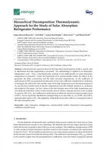
Fig. 3. Top: t for Gau-Seidel factors (left) and Scharfetter-Gummel factors (right). Bottom: t for ILU factors (left) and the hybrid scheme (right). Using the interpolation coecients given in Table 1, we have numerically computed t for the Gau-Seidel, the ILU and the Scharfetter-Gummel factors. AHB fc;av;symm is a rank one matrix only for the ILU factors.

14

R. E. Bank and S. Gutsch

The results are shown in Figure 3. In these gures, t is graphed as a function of ( 1 h; 2 h). In viewing these gures, we note that the ILU scheme seems preferable in most cases; when j jh  0, the convergence rate forpILU approaches one, while that for exponential interpolation approaches 1= 2. Thus we are motivated to suggest a hybrid variant which combines the best properties of these two methods. Let SG and ILU be a pair of corresponding interpolation factors for the SG and ILU schemes. Let F (x) be any continuous, monotonically increasing function on [0; 1) satisfying F (0) = 0, i.e. F (x) = xp for some p > 0 or F (x) = ex ? 1 for some  > 0. De ne a new interpolation factor  by + SG  = F (j Fj (jvj 2j?jv v1?j)vILU j) + 1 2

1

where v1 ; v2 denote the coarse grid vertices between which we want to interpolate. We have a similar formula for all corresponding pairs of interpolation factors. Near j j jv2 ? v1 j = 0, this scheme behaves like the exponential scheme, which is the best scheme for small j j jv2 ? v1 j. On the other hand, when j j jv2 ? v1 j is large, it willx behave like the ILU scheme. Figure 3 (bottom right) shows t for F (x) = e ? 1. 2

6 Analysis for the two-level method In this section we will derive upper bounds for the convergence rate of the generalized hierarchical basis multigrid method (on two levels). The discretization described in section 2 leads to a linear system of equations of the form

ANB x = b:

(15)

If we order the nodal basis functions by level (i.e. rst coarse and then ne), the following block partitioning results for ANB :

ANB =

 ANB ANB 

c cf NB ; ANB fc Af

(16)

where ANB f corresponds to the nodal basis functions of the ne grid nodes, NB Ac corresponds to the ( ne grid) nodal basis functions of the coarse grid NB nodes and ANB cf and Afc correspond to the coupling between the two sets of basis functions. We consider transformations of the form AHB = S T ANB S~, where S and S~ have the block structure  I 0  I 0 ~ S= RI (17) and S = R~ I :

Generalized HBMG

15

By direct calculation, we obtain

 HB NB RT ANB  f S T ANB S~ = ANBA+c ANB R~ Acf + ANB fc f f

where

(18)

NB T NB NB T NB ~ AHB c = Ac + R Afc + Acf R~ + R Af R:

(19) Dierent algorithms are characterized by dierent choices of R and R~ . Our two level iteration is the block symmetric Gau-Seidel iteration. Given a starting vector x0 , the matrix formulation for the remaining iterates is given by xi+1 = xi + W ?1 (b ? Axi ) (20) where W = (D + U )D?1 (D + L), and D, L, and U are the block diagonal, lower triangular, and upper triangular, resp. parts of A. The asymptotic convergence rate of the method is given by the spectral radius (M ) of the iteration matrix M = I ? W ?1 A. Lemma 9. Let A be a regular matrix, let B be a diagonal non-singular matrix and let A = B ?1 AB be a similarity transformation. Let M; M be the iteration matrices for the block symmetric Gau-Seidel iteration (20) applied to A; A. Then (M ) = (M ); i.e. the asymptotic convergence rates for A and A are asymptotically the same. Proof. The proof is straightforward.

Lemma 9 justi es deriving convergence rates for the symmetrized nodal and hierarchical basis stiness matrices since the unsymmetric matrices are symmetrized by a similarity transformation with a non-singular diagonal matrix B . Theorem 10. Let W = B?1WB where W and B are de ned as above, and suppose that < 1 in the strengthened Cauchy inequality. Then the eigenvalues of the generalized eigenvalue problem  = W x Ax lie in the closed interval 1 ? 2    1, and (I ? W ?1 A)  2 < 1. Proof. The proof follows Theorem 6 of [1]. The theorem is an immediate consequence of the estimates T 1 :  1  x TWx  x Ax 1 ? 2

16

R. E. Bank and S. Gutsch

Since W = A + L D ?1 L T (note U = L T ) and L D ?1 L T is symmetric, positive semide nite, it is clear that the lower bound is one. The upper bound is given by 1 +  where xT L D ?1 L T x :  = max T x6=0

x Ax

This can be written as

 yT Dy  = max T  ; x6=0 x Ax

where

 = L T x: Dy

Consider the hierarchical decomposition of V = Vc  Vf . Let a(
;
) be symmetrized bilinear form corresponding to A, and let j vj 2 = a(v; v). Then in nite element notation, we have

j v^j 2 ;  = max u6=0 j uj 2

(21)

where u = v + w, v 2 Vc , w 2 Vf and v^ 2 Vc satis es

a(^v; ) = a(w; )

(22)

for all  2 Vc . Written in nite element language, it is easy to analyse (21)(22) in terms of the strengthened Cauchy inequality. We take  = v^ in (22) to see j v^j  j wj : On the other hand

j uj = j vj + j wj + 2a(v; w)  j vj + j wj ? 2 j vj j wj  (1 ? )j wj  (1 ? ) ? j v^j : 2

2

2

2

2

2

2

2

2

2

The theorem now follows from combining this estimate and (21).

ut

7 Numerical results and conclusions In this section we present numerical results for the interpolation coecients analysed in the previous sections. We apply the schemes to the model convection-diusion equation (1) with f = 1 on = (0; 1)  (0; 1). The problem is discretized using the Scharfetter-Gummel method. We perform experiments for the two-level method where the coarse grid is uniformly re ned by dividing each triangle into four congruent triangles. We use uniform

Generalized HBMG

17

grids with structured re nement in order to treat all cases in a more standardized setting. We illustrate the dependence of the convergence rate on the direction and magnitude of h. We record average rates of convergence after k = minf100; kg iterations, where the residual was reduced by 10?4 in k steps. The average rate of convergence is given by (krk k2 =kr0k2 ) k , where ri denotes the residual after i steps. In the rst table, we also record the improvement in the last step, i.e. krk k2 =krk?1 k2. These values are denoted in brackets. The entry `zero' denotes the occurrence of a zero pivot in the underlying LU-decomposition. We choose x0 = (0; 0;


; 0)T as a starting vector. All calculations were done in double precision on a Sparc10. 1

= 3969 Lin G-S S-G ILU hybrid (0; 0) 0.19 (0.34) 0.99 (0.99) 0.19 (0.34) 0.99 (0.99) 0.19 (0.34) (0; 1000) 0.52 (0.49) 0.74 (0.17) 0.70 (0.08) 0.35 (0.13) 0.35 (0.13) (0; 5000) 0.52 (0.48) 0.69 (0.01) 0.70 (0.09) 0.09 (0.03) 0.09 (0.03) (707; 707) 0.56 (0.56) 0.80 (0.41) 0.82 (0.10) 0.62 (0.17) 0.62 (0.17) (3536; 3536) 0.56 (0.56) 0.80 (0.41) zero (zero) 0.62 (0.17) 0.62 (0.17) (?707; 707) 0.57 (0.63) 0.79 (0.41) 0.51 (0.28) 0.61 (0.17) 0.61 (0.17) (?3536; 3536) 0.57 (0.63) 0.79 (0.41) 0.51 (0.28) 0.61 (0.17) 0.61 (0.17) Table 2. Convergence rates for various two-level methods and for several values of = ( 1 ; 2 )T . (\lin" is linear interpolation, \G-S" is Gau-Seidel, \S-G" is exponential interpolation and \ILU" is ILU interpolation. N

= (0; 1000)T Lin G-S S-G ILU hybrid h = 1=8 (N = 49) 0.45 0.02 0.44 e-3 e-3 h = 1=16 (N = 225) 0.50 0.22 0.45 0.01 0.01 h = 1=32 (N = 961) 0.51 0.56 0.49 0.08 0.08 h = 1=64 (N = 3969) 0.52 0.74 0.70 0.35 0.35 h = 1=128 (N = 16129) 0.53 0.85 0.86 0.63 0.63 = (707; 707)T Lin G-S S-G ILU hybrid h = 1=8 (N = 49) 0.50 e-3 zero e-5 e-5 h = 1=16 (N = 225) 0.56 0.39 zero 0.19 0.19 h = 1=32 (N = 961) 0.56 0.64 0.66 0.36 0.36 h = 1=64 (N = 3969) 0.56 0.80 0.82 0.62 0.62 h = 1=128 (N = 16129) 0.55 0.89 0.90 0.79 0.79 Table 3. Convergence rates for various two-level methods and for several values of h with xed = (0; 1000)T (top) and = (707; 707)T (bottom).

Typical convergence histories are shown in Figure 4, where log kri k=kr0k is plotted as a function of the iteration index i. Here we observe the nonmonotonic behavior of the residual for the Scharfetter-Gummel factors.

18

R. E. Bank and S. Gutsch

The results for the two level method let the linear factors appear very favorable. We point out that this is only the case for two levels. For more than two levels, the method is applied recursively for the calculated coarse grid approximation. Unfortunately, the coarse grid matrix usually does not correspond to a discretization of our model problem (1) on the coarse grid anymore. For linear factors as well as for the Scharfetter-Gummel factors, we obtain seven point formulae describing possibly inde nite systems. For these the above considerations about including the geometry of the mesh or the coecients of the problem into the calculation of the interpolation factors do not apply. Thus it is not surprising that our numerical experiments for these methods for more than two levels usually failed. On the other side, the ILU-factors seem to provide a robust scheme for more than two levels. The resulting coarse grid matrix will be diagonally dominant, and the factors for further unre nement are calculated using the entries of this coarse grid matrix. In our numerical experiments we observed that the convergence rates hardly decreased when switching from two to several levels.

Fig. 4. The initialndmesh (1st) and convergence histories for ILU, = (0; 1000)T , rd

where h = 1=64 (2 ) and h = 1=128 (3 ) .

Fig. 5. Convergence histories with = (0; 1000)T for Scharfetter-Gummel where st nd rd h = 1=64;

(1 ), Gau-Seidel, h = 1=64 (2 ) and Linear, h = 1=64 (3 ).

Generalized HBMG

19

References 1. R. E. Bank, Hierarchical bases and the nite element method, in Acta Numerica 1996 (A. Iserles, ed.), Cambridge University Press, 1996, pp. 1{43. 2. R. E. Bank and M. Benbourenane, The hierarchical basis multigrid method for convection diusion equations, Numerische Mathematik, 61 (1992), pp. 7{ 37. 3. R. E. Bank, J. Burgler, W. Fichtner, and R. K. Smith, Some upwinding techniques for nite element approximations of convection-diusion equations, Numerische Mathematik, 58 (1990), pp. 185{202. 4. R. E. Bank and T. F. Dupont, Analysis of a two level scheme for solving nite element equations, Tech. Rep. CNA-159, Center for Numerical Analysis, University of Texas at Austin, 1980. 5. R. E. Bank, T. F. Dupont, and H. Yserentant, The hierarchical basis multigrid method, Numer. Math., 52 (1988), pp. 427{458. 6. R. E. Bank and S. Gutsch, Hierarchical basis for the convection-diusion equation on unstructured meshes, in Ninth International Symposium on Domain Decomposition Methods for Partial Dierential Equations (P. Bjrstad, M. Espedal and D. Keyes, eds.), J. Wiley and Sons, New York, to appear. 7. R. E. Bank and D. J. Rose, Some error estimates for the box method, SIAM J. Numerical Analysis, 24 (1987), pp. 777{787. 8. R. E. Bank and J. Xu, The hierarchical basis multigrid method and incomplete LU decomposition, in Seventh International Symposium on Domain Decomposition Methods for Partial Dierential Equations (D. Keyes and J. Xu, eds.), AMS, Providence, Rhode Island, 1994, pp. 163{173. 9. , An algorithm for coarsening unstructured meshes, Numerische Mathematik, 73 (1996), pp. 1{36. 10. J. Bramble, J. Pasciak, and J. Xu, The analysis of multigrid algorithms with non-imbedded spaces or non-inherited quadratic forms, Math. Comp., 56 (1991), pp. 1{43. 11. T. F. Chan and B. F. Smith, Domain decomposition and multigrid algorithms for elliptic problems on unstructured meshes, in Proceedings of Seventh International Conference on Domain Decomposition. (ed. D. Keyes and J. Xu), AMS, Providence, Rhode Island, 1994, pp. 175{189. 12. P. M. de Zeeuw and E. J. van Asselt, The convergence rate of multilevel algorithms applied to the convection-diusion equation, SIAM J. Sci. Stat. Comput., 6 (1985), pp. 492{503. 13. V. Eijkhout and P. Vassilevski, The role of the strengthened CauchyBuniakowskii-Schwarz inequality in multilevel methods, SIAM Review, 33 (1991), pp. 405{419. 14. G. H. Golub and C. F. Van Loan, Matrix Computations, Johns Hopkins, 1st ed., 1983. 15. W. Hackbusch, Multigrid convergence for a singular perturbation problem, Lin. Alge. Appl., 58 (1984), pp. 125{145. 16. W. Hackbusch, Multigrid Methods and Applications, Springer-Verlag, Berlin, 1985. 17. W. Hackbusch and S. A. Sauter, A new nite element space for the approximation of pdes on domains with complicated microstructure, tech. rep., Universitat Kiel, 1995.

20

R. E. Bank and S. Gutsch

18. R. Kornhuber and H. Yserentant, Multilevel methods for elliptic problems of domains not resolved by the coarse grid, in Seventh International Symposium on Domain Decomposition Methods for Partial Dierential Equations (D. Keyes and J. Xu, eds.), AMS, Providence, Rhode Island, 1994, pp. 49{60. 19. J. F. Maitre and F. Musy, The contraction number of a class of two level methods; an exact evaluation for some nite element subspaces and model problems, in Multigrid Methods: Proceedings, Cologne 1981 (Lecture Notes in Mathematics 960), Springer-Verlag, Heidelberg, 1982, pp. 535{544. 20. E. J. van Asselt, The multigrid method and arti cial viscosity, in Multigrid Methods: Proceedings, Cologne 1981 (Lecture Notes in Mathematics 960), Springer-Verlag, Heidelberg, 1982, pp. 313{327. 21. H. Yserentant, Hierarchical bases of nite element spaces in the discretization of nonsymmetric elliptic boundary value problems, Computing, 35 (1985), pp. 39{49. 22. , On the multi-level splitting of nite element spaces, Numer. Math., 49 (1986), pp. 379{412.