The GraphPad guide to comparing dose-response or kinetic curves. Dr. Harvey Motulsky President, GraphPad Software Inc.
[email protected] www.graphpad.com Copyright © 1998 by GraphPad Software, Inc. All rights reserved. You may download additional copies of this document from www.graphpad.com, along with companion booklets on nonlinear regression, radioligand binding and statistical comparisons. This article was published in the online journal HMS Beagle, so you may cite: Motulsky, H. Comparing dose-response or kinetic curves with GraphPad Prism.
In HMS Beagle: The BioMedNet Magazine
(http://hmsbeagle.com/hmsbeagle/34/booksoft/softsol.htm) Issue 34. July 10, 1998.
GraphPad Prism and InStat are registered trademarks of GraphPad Software, Inc. To contact GraphPad Software:
10855 Sorrento Valley Road #203 San Diego CA 92121 USA Phone: 619-457-3909 Fax: 619-457-3909 Email:
[email protected] Web: www.graphpad.com
July 1998
Introduction Statistical tests are often used to test whether the effect of an experimental intervention is statistically significant. Different tests are used for different kinds of data – t tests to compare measurements, chi-square test to compare proportions, the logrank test to compare survival curves. But with many kinds of experiments, each result is a curve, often a dose-response curve or a kinetic curve (time course). This article explains how to compare two curves to determine if an experimental intervention altered the curve significantly. When planning data analyses, you need to pick an approach that that matches your experimental design and whose answer best matches the biological question you are asking. This article explains six approaches. In most cases, you’ll repeat the experiment several times, and then want to analyze the pooled data. The first step is to focus on what you really want to know. For dose-response curves, you may want to test whether the two EC50 values differ significantly, whether the maximum responses differ, or both. With kinetic curves, you’ll want to ask about differences in rate constants or maximum response. With other kinds of experiments, you may summarize the experiment in other ways, perhaps as the maximum response, the minimum response, the time to maximum, the slope of a linear regression line, etc. Or perhaps you want to integrate the entire curve and use area-under-the-curve as an overall measure of cumulative response. Once you’ve summarized each curve as a single value either using nonlinear regression (approach 1) or a more general method (approach 2), compare the curves using a t test. If you have performed the experiment only once, you’ll probably wish to avoid making any conclusions until the experiment is repeated. But it is still possible to compare two curves from one experiment using approaches 3-6. Approaches 3 and 4 require that you fit the curve using nonlinear regression. Approach 3 focuses on one variable and approach 4 on comparing entire curves. Approach 5 compares two linear regression lines. Approach 6 uses two-way ANOVA to compare curves without the need to fit a model with nonlinear regression, and is useful when you have too few doses (or time points) to fit curves. This method is very general, but the questions it answers may not be the same as the questions you asked when designing the experiment. This flow chart summarizes the six approaches:
GraphPad Guide to Comparing Curves.
Page 2 of 13
Have you perfromed the experiment more than once?
Yes
Can you fit the data to a model with linear or nonlinear regression?
Yes
Œ
No
•
Variable
Ž
Curve
•
No, Once Can you fit the data to a model with linear regression, nonlinear regression, or neither?
Nonlin
Do you care about a single best-fit variable? Or do you want to compare the entire curves? Linear Neither
• ‘
Approach 1. Pool several experiments using a best-fit parameter from nonlinear regression The first step is to fit each curve using nonlinear regression, and to tabulate the bestfit values for each experiment. Then compare the best-fit values with a paired t test. For example, here are results of a binding study to determine receptor number (Bmax). The experiment was performed three times with control and treated cells side-by-side. Here are the data: Experiment 1 2 3
Bmax (sites/cell) Control 1234 1654 1543
Bmax (sites/cell) Treated 987 1324 1160
Because the control and treated cells were handled side-by-side, analyze the data using a paired t test. Enter the data into GraphPad InStat, GraphPad Prism (or some other statistics program) and choose a paired t test. The program reports that the two-tailed P value is 0.0150, so the effect of the treatment on reducing receptor number is statistically significant. The 95% confidence interval of the decrease in receptor number ranges from 149.70 to 490.30 sites/cell. If you want to do the calculations by hand first compute the difference between Treated and Control for each experiment. Then calculate the mean and SEM of those differences. The ratio of the mean difference (320.0) divided by the SEM of the differences (39.57) equals the t ratio (8.086). There are 2 degrees of freedom (number of experiments minus 1). You could then use a statistical table to determine that the P value is less than 0.05.
GraphPad Guide to Comparing Curves.
Page 3 of 13
The nonlinear regression program also determined Kd for each curve (a measure of affinity), along with the Bmax. Repeat the paired t test with the Kd values if you are also interested in testing for differences in receptor affinity. (Better, compare the log(Kd) values, as the difference between logs equals the log of the ratio, and it is the ratio of Kd values you really care about.) These calculations were based only on the best-fit values from each experiment, ignoring all the other results calculated by the curve-fitting program. You may be concerned that you are not making best use of the data, since the number of points and replicates do not appear to affect the calculations. But they do contribute indirectly. You’ll get more accurate fits in each experiment if you use more concentrations of ligand (or more replicates). The best-fit results of the experiments will be more consistent, which increases your power to detect differences between control and treated curves. So you do benefit from collecting more data, even though the number of points in each curve does not directly enter the calculations. One of the assumptions of a t test is that the uncertainty in the best-fit values follows a bell-shaped (Gaussian) distribution. The t tests are fairly robust to violations of this assumption, but if the uncertainty is far from Gaussian, the P value from the test can be misleading. If you fit your data to a linear equation using linear regression or polynomial regression, this isn’t a problem. With nonlinear equations, the uncertainty may not be Gaussian. The only way to know whether the assumption has been violated is to simulate many data (with random scatter), fit each simulated data set, and then examine the distribution of best-fit values. With reasonable data (not too much scatter), a reasonable number of data points, and equations commonly used by biologists, the distribution of best-fit values is not likely to be far from Gaussian. If you are worried about this, you could use a nonparametric MannWhitney test instead of a t test.
Approach 2. Pool several experiments without nonlinear regression With some experiments you may not be able to choose a model, so can’t fit a curve with nonlinear regression. But even so, you may be able to summarize each experiment with a single value. For example, you could summarize each curve by the peak response, the time (or dose) to peak, the minimum response, the difference between the maximum and minimum responses, the dose or time required to increase the measurement by a certain amount, or some other value. Pick a value that matches the biological question you are asking. One particularly useful summary is the area under the curve, which quantifies cumulative response. Once you have summarized each curve as a single value, compare treatment groups with a paired t test. Use the same computations shown in approach 1, but enter the area under the curve, peak height, or some other value instead of Bmax .
GraphPad Guide to Comparing Curves.
Page 4 of 13
Approach 3. Analyze one experiment with nonlinear regression. Compare best-fit values of one variable. Even if you have only performed the experiment only once, you can still compare curves with a t test. A t test compares a difference with the standard error of that difference. In approaches 2 and 3, the standard error was computed by pooling several experiments. With approach 3, you use the standard error reported by the nonlinear regression program. For example, in the first experiment in Approach 1, Prism reported these results for Bmax: Control Treated
Best-fit Bmax 1234 987
SE 98 79
df 14 14
You can compare these values, obtained from one experiment, with an unpaired t using InStat or Prism (or any statistical program that can compute t tests from averaged data). Which values do you enter? Enter the best-fit value of the Bmax as “mean” and the SE of the best-fit value as “SEM”. Choosing a value to enter for N is a bit tricky. The t test program really doesn’t need sample size (N). What it needs is the number of degrees of freedom, which it computes as N-1. Enter “N=15” into the t test program for each group. The program will calculate DF as N-1, so will compute the correct P value. The two-tailed P value is 0.0597. Using the conventional threshold of P=0.05, the difference between Bmax values in this experiment is not statistically significant. To calculate the t test by hand, calculate 1234 - 987 = 1.962 t= 98 2 + 79 2 The numerator is the difference between best-fit Bmax values. The denominator is the standard error of that difference. Since the two experiments were done with the same number of data points, this equals the square root of the sum of the square of the two SE values. If the experiments had different numbers of data points, you’d need to weight the SE values so the SE from the experiment with more data (more degrees of freedom) gets more weight. You’ll find the equation in reference 1 (applied to exactly this problem) or in almost any statistics book in the chapter on unpaired t tests. The nonlinear regression program states the number of degrees of freedom for each curve. It equals the number of data points minus the number of variables fit by nonlinear regression. In this example, there were eight concentrations of radioligand in duplicate, and the program fits two variables (Bmax and Kd). So there were 8*2 – 2 or 14 degrees of freedom for each curve, so 28 df in all. You can find the P value from an appropriate table, a program such as StatMate, or by typing this equation into an empty cell in Excel =TDIST(1.962, 28, 2) . The first parameter is
GraphPad Guide to Comparing Curves.
Page 5 of 13
the value of t; the second parameter is the number of df, and the third parameter is 2 because we want a two-tailed P value. Prism reports the best-fit value for each parameter along with a measure of uncertainty, which it labels the standard error. Some other programs label this the SD. When dealing with raw data, the SD and SEM are very different – the SD quantifies scatter, while the SEM quantifies how close your calculated (sample) mean is likely to be to the true (population) mean. The SEM is the standard deviation of the mean, which is different than the standard deviation of the values. When looking at best-fit values from regression, there is no distinction between SE and SD. So even if your program labels the uncertainty value “SD”, you don’t need to do any calculations to convert it to a standard error.
Approach 4. Analyze one experiment with nonlinear regression. Compare entire curves. Approach 3 requires that you focus on one variable that you consider most relevant. If you care about several variables, you can repeat the analysis with each variable fit by nonlinear regression. An alternative is to compare the entire curves. Follow this approach. 1. Fit the two data sets separately to an appropriate equation, just like you did in Approach 3. 2. Total the sum-of-squares and df from the two fits. Add the sum-of-squares from the control data with the sum-of-squares of the treated data. If your program reports several sum-of-squares values, sum the residual (sometimes called error) sum-of-squares. Also add the two df values. Since these values are obtained by fitting the control and treated data separately, label these values, SSseparate and DFseparate. For our example, the sums-of-squares equal 1261 and 1496 so SSseparate equals 2757. Each experiment had 14 degrees of freedom, so DFseparate equals 28. 3. Combine the control and treated data set into one big data set. Simply append one data set under the other, and analyze the data as if all the values came from one experiment. Its ok that X values are repeated. For the example, you could either enter the data as eight concentrations in quadruplicate, or as 16 concentrations in duplicate. You’ll get the same results either way, , provided that you configure the nonlinear regression program to treat each replicate as a separate data point. 4. Fit the combined data set to the same equation. Call the residual sum-of-squares from this fit SScombined and call the number of degrees of freedom from this fit DFcombmined. For this example, SScombined is 3164 and DFcombmined is 30 (32 data points minus two variables fit by nonlinear regression). 5. You expect SSseparate to be smaller than SScombined even if the treatment had no effect simply because the separate curves have more degrees of freedom. If the two data sets are really different, then the pooled curve will be far from most of the data and SScombined will be much larger than SSseparate. The question is whether GraphPad Guide to Comparing Curves.
Page 6 of 13
the difference between SS values is greater than you’d expect to see by chance. To find out, compute the F ratio using the equation below, and then determine the corresponding P value (there are DFcombined-DFseparate degrees of freedom in the numerator and DFseparate degrees of freedom in the denominator.
(SS
combined
F=
− SSseparate )
(DF
combined
− DFseparate )
SSseparate DFseparate
For the example, F=2.067 with 2 df in the numerator and 28 in the denominator. To find the P value, use a program like GraphPad StatMate, find a table in a statistics book, or type this formula into an empty cell in Excel =FDIST(2.067,2,28) . The P value is 0.1463. The P value tests the null hypothesis that there is no difference between the control and treated curves overall, and any difference you observed is due to chance. If the P value were small, you would conclude that the two curves are different – that the experimental treatment altered the curve. Since this method compares the entire curve, it doesn’t help you focus on which parameter(s) differ between control and treated (unless, of course, you only fit one variable). It just tells you that the curves differ overall. If you want to focus on a certain variable, such as the EC50 or maximum response, then you should use a method that compares those variables. Approach 4 compares entire curves, so the results can be hard to interpret. In this example, the P value was fairly large, so we conclude that the treatment did not affect the curves in a statistically significant manner.
Approach 5. Compare linear regression lines If your data form straight lines, you can fit your data using linear regression, rather than nonlinear regression. JH Zar discusses how to compare linear regression lines in reference 2. Here is a summary of his approach: First compare the slopes of the two linear regression lines using a method similar to approach 3 above. Pick a threshold P value (usually 0.05) and decide if the difference in slopes is statistically significant. •
If the difference between slopes is statistically significant, then conclude that the two lines are distinct. If relevant, you may wish to calculate the point where the two lines intersect.
•
If the difference between slopes is not significant then fit new regression lines but with the constraint that both must share the same slope. Now ask whether the difference between the elevation of these two parallel lines is statistically significant. If so, conclude that the two lines are distinct, but parallel. Otherwise conclude that the two lines are statistically indistinguishable.
GraphPad Guide to Comparing Curves.
Page 7 of 13
The details are tedious, so aren’t repeated here. Refer to the references, or use GraphPad Prism, which compares linear regression lines automatically. An alternative approach to compare two linear regression lines is to use multiple regression, using a dummy variable to denote treatment group. This approach is explained in reference 3, which also describes, in detail, how to compare slopes and intercepts without multiple regression.
Approach 6. Comparing curves with ANOVA If you don’t have enough data points to allow curve fitting, or if you don’t want to choose a model (equation), you can analyze the data using two-way analysis of variance (ANOVA) followed by posttests. This method is also called two-factor ANOVA (one factor is dose or time; the other factor is experimental treatment). Here is an example, along with the two-way ANOVA results from Prism. Dose 0.0 1.0 2.0
Y1 23.0 34.0 43.0
Control Y2 Y3 25.0 29.0 41.0 37.0 47.0 54.0
Y1 28.0 47.0 65.0
Treated Y2 Y3 31.0 26.0 54.0 56.0 60.0
Response
75 50 25
Control Treated
0 0
1
2
Dose Source of Variation Interaction Treatment Dose Source of Variation Interaction Treatment Dose Residual
Df 2 1 2 11
P value 0.0384 0.0002 P