25 teger entries. Conrad [1] demonstrates that the group can be generated with. 26 .... a Pythagorean triple. However, there exist no primitive Pythagorean triples.
Open Systems & Information Dynamics Vol. 19, No. 1 (2012) 1–28 DOI: xxx c World Scientific Publishing Company ⃝
1
The Group of Dyadic Unitary Matrices
2
Alexis De Vos, Rapha¨el Van Laer, and Steven Vandenbrande
5
Vakgroep elektronica en informatiesystemen Universiteit Gent Sint Pietersnieuwstraat 41, B–9000 Gent, Belgium
6
(Received: September 2, 2011)
3 4
7 8 9 10 11 12 13 14
15
16 17
Abstract. We introduce the group DU(m) of m × m dyadic unitary matrices, i.e. unitary matrices with all entries having a real and an imaginary part that are both rational numbers with denominator of the form 2p (with p a non-negative integer). We investigate in detail the finite groups DU(1) and DU(2) and the discrete, but infinite groups DU(3) and DU(4). We further introduce the subgroup XDU(m) of DU(m), consisting of those members of DU(m) that have constant line sum 1. The study of XDU(2) and XDU(4) leads to conclusions concerning the synthesis of quantum computers acting on one and two qubits, respectively.
1.
Introduction
Basically, there exist three kinds of groups: • finite groups, i.e. groups with a finite order,
19
• infinite but nevertheless discrete groups, i.e. groups with a countably infinite order, and
20
• Lie groups, i.e. groups with an uncountably infinite order.
18
21 22 23 24 25 26 27 28 29 30 31 32 33
Whereas the size of a finite group is quantified by its order, the size of a Lie group is quantified by its dimensionality. Quantifying sizes of infinite discrete groups is a more difficult task. It necessitates a detailed study of the group. The most basic example of a countably infinite nonabelian group is the discrete group SL2 (Z), i.e. the special linear group of 2 × 2 matrices with integer entries. Conrad [1] demonstrates that the group can be generated with merely two generators and shows how to decompose an arbitrary group member into a finite product of factors, each equal to one of these two building blocks. In the present paper, we follow a basically similar approach for describing the group of rational unitary matrices where all matrix elements have a denominator of the form 2p . The motivation to study this group is inspired by its importance in computer theory. Whereas classical reversible computation is described by finite groups and quantum computation is represented by
2 34 35 36 37 38 39
A. De Vos, R. Van Laer, and S. Vandenbrande
Lie groups, computing with the so-called square-root-of-NOT logic gate leads to infinite discrete groups [2] of such rational matrices. Whereas classical reversible circuits are generated by controlled NOT gates (a.k.a. Toffoli gates), below we will investigate all circuits generated by controlled square roots of NOT. They constitute a generalization of the classical reversible circuits, but only a small fraction of the set of all quantum circuits. 2.
40
41 42 43 44 45 46 47
48 49 50 51 52 53 54 55 56 57 58
59 60 61 62 63 64
First, we consider all unitary m × m matrices. It is well known that they form an infinite group, i.e. the unitary group U(m), an m2 -dimensional Lie group. Next, we consider, within the group U(m), the matrices which have exclusively Gaussian entries. This means that the matrix entries are Gaussian rationals a b c d +i , + i , ... , A B C D where a, A, b, B, . . . are integers. These matrices form a group. Indeed, being unitary, such matrix has an inverse. The entries of the inverse automatically are also Gaussian rationals. And the product of two such matrices automatically is also such a matrix. We call this group the Gaussian unitary group GU(m). The group is discrete, as the matrix contains only a finite number (i.e. 2m2 ) of rational numbers Aa , Bb , . . . and there exist only a countably infinite number of rationals. Finally, within the group GU(m), we consider the subset of matrices where all denominators A, B, . . . are a power of 2. Thus all entries may be written a b +i p , 2p 2 where the non-negative integer p is chosen such that at least one entry is not reducible, i.e. such that at least one of the 2m2 numerators a, b, . . . is odd. As the real part and the imaginary part of each matrix entry is a dyadic rational, we call such a matrix a dyadic matrix. Whereas m is called the dimension (or degree) of the matrix, the number 2p is called the level [3] of the matrix. As illustrated by the example (
65
66 67 68 69
The Group DU(m)
5 2 1 2
1 1 2
)−1
( =
2 3 − 23
− 43 10 3
) ,
the inverse of a dyadic matrix is not necessarily a dyadic matrix. The inverse of dyadic unitary matrix, however, is a dyadic unitary matrix (with the same level), for the simple reason that the inverse of a unitary matrix is its Hermitian transpose. The product of a dyadic matrix with level equal to 2p1 and a
The Group of Dyadic Unitary Matrices 70 71 72
73
3
dyadic matrix with level equal to 2p2 is a dyadic matrix with level lower than or equal to 2p1 +p2 . We thus may conclude that the dyadic unitary matrices form a group. We call this group the dyadic unitary group DU(m). 3.
Two Subgroups of DU(m)
103
In the present section, we discuss two (out of the many) subgroups of DU(m). An m × m matrix has 2m lines, i.e. m rows and m columns. We consider the matrices whose line sums are all equal. If the matrix is unitary, then the constant line sum is on the unit circle (See Appendix A). If the matrix is dyadic, then the constant line sum is a dyadic rational. Now, on the unit circle there exist only four such Gaussian rationals 2xp + i 2yp . Indeed, the condition ( 2xp )2 + ( 2yp )2 = 1 leads to x2 + y 2 = (2p )2 , which implies that {x, y, 2p } forms a Pythagorean triple. However, there exist no primitive Pythagorean triples where the greatest number is even. We conclude that either x or y has to be zero. Therefore, if the matrix is both unitary and dyadic, the constant line sum equals one of the four complex numbers 1, i, −1, and −i, known as the four Gaussian units. The product of a matrix with constant line sum equal to s and a matrix with constant line sum equal to t is a matrix with constant line sum st. Proof is provided in [4, p. 239]. Therefore, matrices with constant line sum equal to 1 form a group. The members of DU(m) that have constant line sum equal to 1, thus form a subgroup of DU(m); we will call this subgroup XDU(m). Their study is interesting in the framework of quantum computing. The groups XDU(2w ) naturally appear when studying quantum circuits built with the gate called ‘the square root of NOT’, see below in Sections 8 to 11. Matrices belonging to XDU(m) may be considered as a ‘complex generalization’ of doubly stochastic (or bistochastic) matrices, where equally well all line sums equal 1, but where all entries are restricted to real non-negative numbers. The matrices of DU(m) with p = 0, i.e. the DU(m) matrices of level 1, form a finite subgroup, isomorphic to the semi-direct product (DU(1) × DU(1) × . . . × DU(1)): S m = DU(1)m : S m , where S m denotes the symmetric group of degree m (and thus order m!). We will call the subgroup the monomial dyadic unitary group MDU(m), as all its members are matrices with exactly one non-zero entry in each row and each column. The group P(m) of all m × m permutation matrices, in turn, is a subgroup of MDU(m):
104
P(m) ⊂ MDU(m) ⊂ DU(m) ⊂ U(m) .
74 75 76 77 78 79 80 81 82 83 84 85 86 87 88 89 90 91 92 93 94 95 96 97 98 99 100 101 102
105 106 107 108
The subgroup MDU(m) partitions the supergroup DU(m) into double cosets, each containing matrices of a same level 2p . These double cosets can be regarded as equivalence classes. Any element of a double coset can act as its representative. Here, two matrices are considered equivalent iff they can
4 109 110
A. De Vos, R. Van Laer, and S. Vandenbrande
be converted into one another by applying a combination of the following operations:
111
• permutation of two rows or two columns and
112
• multiplication of a row or a column by i.
113 114
115
116 117 118 119 120 121 122
123
124
125
This equivalence is analogous to the one used in investigating real and complex Hadamard matrices. See e.g. the equivalence relation ≈ by Haagerup [5]. 4.
The Group DU(1) and its subgroup XDU(1)
The group DU(1) is the group of Gaussian numbers 2ap + i 2bp , such that ( 2ap )2 +( 2bp )2 = 1. As demonstrated in the previous section, only the numbers ±1 and ±i satisfy this condition. Thus DU(1) is isomorphic to the finite group of the four complex numbers 1, i, −1, and −i. This group has order 4 and is isomorphic to the cyclic group Z 4 . The subgroup MDU(1) is identical to DU(1). The subgroup XDU(1) has order 1 and is isomorphic to Z 1 . 5.
The Group DU(2) and its Subgroup XDU(2)
We consider the unitary matrices of the form ( ) b c d a + i + i p p p p 2 2 2 2 e 2p
+ i 2fp
g 2p
+ i 2hp
,
127
where at least one of the eight integers a, b, c, . . . , h is odd. For the sake of convenience, we assume that {a, b, c, d} contains an odd number. We have
128
a2 + b2 + c2 + d2 = 4p .
126
(1)
131
According to Lagrange’s theorem each natural number can be written as the sum of four squares. So can 4p . If p = 0, then only one partition into four squares exists:
132
1 = 12 + 0 2 + 0 2 + 0 2 .
129 130
133 134 135
136 137
(2)
If p > 0, then (1) implies that a2 + b2 + c2 + d2 has to be a multiple of 4. Therefore, either all four numbers a, b, c, and d are even or all are odd. If p = 1, then both kinds of partition exist: 4 = 12 + 12 + 12 + 12 = 22 + 02 + 02 + 02 .
(3)
The Group of Dyadic Unitary Matrices 138
If p > 1, then the four numbers are necessarily even: 4p = (2p−1 )2 + (2p−1 )2 + (2p−1 )2 + (2p−1 )2 = (2p )2 + 02 + 02 + 02 .
139 140
141 142 143 144 145 146 147 148 149
150
5
We denote by ps (n) the number of partitions of a number n into s squares. In contrast to this number of partitions, the total number of representations of the number n as a sum of s squares takes into account order and sign of the parts, thus e.g. considering 4 = 22 +02 +02 +02 , 4 = 02 +22 +02 +02 , and 4 = (−2)2 + 02 + 02 + 02 as three different solutions of a2√+ b2 + c2 + d2 = 4. This number of ‘lattice on the hypersphere with radius n ’ traditionally is denoted rs (n). We have (for n > 0 and s > 3) that rs (n) ≫ ps (n). Thanks to Jacobi [6], explicit expressions [7, 8, 9] exist for r2 (n), r4 (n), r6 (n), r8 (n), and r12 (2n). In particular, we have ∑ r4 (n) = 8 d, 4̸ | d | n
151
yielding r4 (4 ) =
152
153
154
155 156 157 158 159 160 161 162 163 164
165
{ p
As a result, we have
{ p4 (4p ) =
8 24
if if
p=0 p > 0.
1 2
if if
p=0 p > 0.
(4)
Thus there exist no other partitions of 4p than those mentioned above. As a result, there exists no partition a2 + b2 + c2 + d2 of 4p (with p > 1) with at least one odd number a, b, c, or d. That is the reason why there do not exist any dyadic unitary 2×2 matrices with p ≥ 2. The fact that neither p4 (4p ) nor r4 (4p ) increase for increasing p, once p ≥ 1, explains why no dyadic unitary 2 × 2 matrices with p > 1 exist. We conclude that the group DU(2) consists of matrices with level equal to either 1 or 2. As a consequence, the group is finite. It consists of the Gaussian unitary matrices where either all denominators are 1 (and numerators are based on (2)) or all denominators are 2 (and numerators are based on (3)): ( ( ) ( ) ) 1 α 0 a + ib c + id 0 α or , or 0 β β 0 2 e + if g + ih where α and β are 1, i, −1, or −i and a, b, . . ., and h are 1 or −1. This yields a group of order 96. Its most notorious members are ( ( ) ) ( ) 1 1+i 1−i 1 0 0 1 , , and 0 1 1 0 2 1−i 1+i
6
A. De Vos, R. Van Laer, and S. Vandenbrande
175
representing, in quantum computation, the dummy gate, the NOT gate [10, 4], and the square root of NOT gate [2, 10, 4, 11, 12, 13], respectively. The group is isomorphic to the group [96, 67] of the GAP library. It consists of 32 matrices with p = 0 and 64 matrices with p = 1. The former constitute the subgroup MDU(2), isomorphic to (DU(1) × DU(1)) : S 2 and thus to Z 24 : Z 2 . The subgroup MDU(2) partitions the supergroup DU(2) into two double cosets, one containing all the matrices with p = 0, the other all the matrices with p = 1. Besides the permutation group P(2), also the Pauli group [14, 15] P is a subgroup of MDU(2):
176
P(2) ⊂ P ⊂ MDU(2) ⊂ DU(2) ⊂ U(2) ,
166 167 168 169 170 171 172 173 174
177
178
179 180 181 182 183
184
185
186
187 188
with successive orders 4 < 16 < 32 < 96 < ∞4 . According to the definition in Sect. 3, the members of DU(2) with all four line sums equal to 1, form the subgroup XDU(2) of DU(2). The subgroup has order 4. Only two of the four matrices of XDU(2) belong to MDU(2). The subgroup XDU(2) partitions its supergroup DU(2) into nine double cosets, five of size 16 and four of size 4. 6.
The Group DU(3)
For the case m = 3, we have to investigate a partition into six squares: a2 + b2 + c2 + d2 + e2 + f 2 = 4p with at least one of the integers {a, b, c, d, e, f } odd. Whatever the value of p, such partition is possible. Suffice it to successively
189
• choose an arbitrary odd number a such that a2 ≤ 4p ,
190
• choose an arbitrary number b such that b2 ≤ 4p − a2 , and
191
• apply Lagrange’s four-square theorem to the number 4p − a2 − b2 .
192
193
194 195 196 197
There always exists at least one partition of the form 4p = 12 + 02 + c2 + d2 + e2 + f 2 . As p can have any value from {0, 1, 2, . . .}, this yields a (countably) infinite number of possibilities. This fact constitutes the underlying reason why DU(3) (in contrast to DU(2)) is a (countably) infinite group. An actual proof of the infinitude of DU(3) is given in Appendix B.
The Group of Dyadic Unitary Matrices 198 199
200
7
The numbers p6 (4p ) and r6 (4p ) grow fast with increasing p. Indeed, according to Jacobi, we have ) ( 4n2 ∑ 2 − d . r6 (n) = 4 (−1)(d−1)/2 d2 2̸ | d | n
201
202
203 204 205 206 207 208 209
210
211 212 213 214 215 216 217 218
219
220
221
222 223 224 225 226
227
For n = 4p this yields r6 (4p ) = 4 (4 × 16p − 1) , i.e. an exponentially increasing function of p, in strong contrast to (4). Within the infinite group DU(3), the matrices with p = 0 form the finite subgroup MDU(3), isomorphic to (DU(1) × DU(1) × DU(1)) : S 3 , of order 43 × 3! = 384. It partitions the whole group into an infinite number of double cosets. All elements of such a double coset have a same value of p. However, two matrices with a same p may be member of two different double cosets. E.g. the two matrices ( ) ( ) 1 1 + 2i 3 − i −3 + i 1 + i 2 1 1 −3 − 2i 1 1+i 1 + i −3 + i 2 and 2 22 2 1−i −1 − 3i 2 2 2 2 + 2i sit in two different double cosets, both with p = 2. The former double coset contains matrices, where all lines (i.e. rows and columns) are based on the partition 16 = 32 + 22 + 12 + 12 + 12 + 02 . The latter double coset contains matrices where four lines are based on this partition, but two other lines are based on 16 = 22 + 22 + 22 + 22 + 02 + 02 . The two double cosets have different size: the former contains 36,864 = 96 × 384 elements, whereas the latter contains only 18,432 = 48 × 384 elements. For large values of n, we have ps (n) ≈
rs (n) , s! 2s
such that, for sufficiently large p, we have p6 (4p ) ≈
1 16p . 2880
The fact that p6 (4p ) grows so rapidly with increasing p leads to a fast growing number of double cosets as a function of the level 2p . For p = 1, we have two double cosets; for p = 2, we have six double cosets; and for p = 3, we have at least seven double cosets. The two double cosets with p = 1 have e.g. the following representatives: ( ( ) ) 2 0 0 0 1−i 1+i 1 1 0 1+i 1−i 1+i 1 −i r1 = and r2 = , 2 2 0 1−i 1+i 1−i i 1
8
A. De Vos, R. Van Laer, and S. Vandenbrande
Table 1: Number of DU(m) matrices.
m=1
m=2
m=3
m=4
p=0
q=0
4
32
384
6,144
p=1 p=1
q=1 q=2
0 0
64 0
2,304 9,216
147,456 5,701,632
p=2 p=2
q=3 q=4
0 0
0 0
36,864 147,456
p=3 p=3
q=5 q=6
0 0
0 0
589,824 2,359,296
4
96
ℵ0
...
... total
ℵ0
230
respectively. It turns out to be advantageous to decompose the number 2 into the irreducible elements of the Gaussian integers,
231
2 = −i(1 + i)2 ,
228 229
232 233
234
235 236 237 238 239 240 241 242 243 244 245
where −i is one of the four Gaussian units (i.e. 1, i, −1, and −i) and 1 + i is a Gaussian prime. We thus obtain ( ) ( ) 1+i 0 0 0 1 + i i(1 + i) 1 1 0 i 1 , r2 = i(1 + i) i 1 r1 = . 1+i (1 + i)2 0 1 i 1+i −1 i We may say that r1 is of level 1+i, whereas r2 is of level (1+i)2 . In this sense, the matrices of level 2p consist of the union of the matrices of level (1 + i)2p−1 and the matrices of level (1 + i)2p . We may say that the Gaussian prime 1 + i plays a role like ‘some kind of rational square root of 2’, thus allowing levels resembling a ‘halfinteger power of 2’. We will use χ as a short-hand notation for 1 + i. We will make use of the following property of the number χ: any Gaussian integer is either 0 mod χ or 1 mod χ. A Gaussian number a + ib is 0 mod χ iff either both a and b are even or both a and b are odd. The number of DU(3) matrices of different levels χq are given in Table 1. All matrices of level χ0 are members of MDU(3), a group isomorphic to DU(1)3 : S 3 of order 43 ×3! = 384. All 3×3 matrices of level χ1 consist of a 1×
9
The Group of Dyadic Unitary Matrices 246 247 248 249 250 251 252 253
254
1 DU(1) block (4 possible contents) and a 2×2 DU(2) block (64 possibilities), with 9 possible block placings: indeed we have 9 × (4 × 64) = 2, 304. All matrices of level χ2 or higher do not fall apart into blocks. Table 1 reveals that, for q > 0, the number of DU(3) matrices with level χq equals 576 × 4q . Appendix C explains why. For p > 0, the DU(3) matrices of level 2p consist of the matrices of levels χ2p−1 and χ2p . Thus (for p > 0) there are 720 × 16p such matrices. An arbitrary matrix A of DU(3) of level χq looks like ( ) a + ib c + id e + if 1 g + ih j + ik l + im A = q (5) χ n + io p + iq r + is
258
with at least one of the nine entries a + ib, c + id, . . ., or r + is not divisible by χ. We now introduce the matrix Rn (A), where n is a Gaussian integer. It is obtained by multiplying A by its level χq and subsequently computing the remainder when dividing each matrix entry by n:
259
Rn (A) = (χq A) mod n .
255 256 257
260
261
E.g. [ Rχ [
262
R2
1 (1 + i)5 1 (1 + i)5
(
(
4 + 2i 1 − 3i −1 − i −1 + 3i −3 −3 + 2i 1−i 2 + 3i −4 − i 4 + 2i 1 − 3i −1 − i −1 + 3i −3 −3 + 2i 1−i 2 + 3i −4 − i
)]
( =
)]
( =
0 0 0 0 1 1 0 1 1
)
0 1+i 1+i 1+i 1 1 1+i i i
) .
266
Note that all entries of an Rχ matrix are either 0 or 1 and all entries of an R2 matrix are 0, 1, i, or 1 + i. For any Gaussian integer n, we have nn mod χ = n mod χ. Therefore, the unitarity condition
267
a2 + b2 + c2 + d2 + e2 + f 2 = 2q ,
263 264 265
268
269
270 271 272
273
in case q > 0, leads to (a + ib) mod χ + (c + id) mod χ + (e + if ) mod χ = 0 and similar for the remaining two rows, as well as for the three columns. Taking also orthogonalities into account, we can conclude that the Rχ matrix of a DU(3) matrix (of level higher than 1) always is of the type ( ) 0 0 0 0 1 1 (6) 0 1 1
10 274 275 276
277
278
279
280 281 282 283 284 285 286 287 288 289 290 291
292
293 294
295
296
297
298
299
A. De Vos, R. Van Laer, and S. Vandenbrande
or equivalent, i.e. of this type after permutation of rows or permutation of columns. One can similarly demonstrate that the R2 matrix of a DU(3) matrix (of level higher than χ1 ) always is of the following type or equivalent: ( ) 0 1+i 1+i 1+i , (7) M 1+i where the lower-right submatrix M exists in five flavours: ( ) ( ) ( ) ( ) ( ) 1 1 1 1 1 i 1 i i i , , , and . 1 1 i i 1 i i 1 i i They correspond to the five 2 × 2 matrices G1 , G2 , . . ., and G5 discussed in Appendix D. By multiplying the DU(3) matrix of level χq by an appropriate DU(3) matrix of level χ, it always is possible to obtain a matrix of level χq−1 (instead of level χq+1 , as one would expect normally). By performing such a multiplication again and again, we can thus lower the level of the matrix from χq to χq−1 , to χq−2 , . . ., to χ0 . It suffices to proceed, at each of the q stages, in three steps: • First, one multiplies by an appropriate permutation matrix (automatically of level 1), such that the original Rχ matrix is converted into the standard form (6). • Next, one either or not multiplies by the diagonal matrix (of level 1) ( ) 1 0 0 0 −i 0 . b = 0 0 1 Detailed study [16] demonstrates that the b matrix has to be applied if the R2 matrix (7) contains the submatrix ( ) ( ) ( ) 1 1 1 1 i i , or 1 1 i i i i and the b matrix should not be applied if the submatrix is ( ) ( ) 1 i 1 i either or . 1 i i 1 • Finally, one right-multiplies by the matrix (of level χ) ( ( ) ) 2 0 0 1+i 0 0 1 1 0 1−i 1+i 0 −i 1 a = = . 2 1+i 0 1+i 1−i 0 1 −i
11
The Group of Dyadic Unitary Matrices 300 301
302
303
304
The second and the third step of the procedure are illustrated by an example where we lower the level of a given matrix from χ5 to χ4 : 4 + 2i 1 −1 + 3i (1 + i)5 1−i
1 − 3i −3 2 + 3i
−1 − i 3−i 1 1 + 2i −3 + 2i ba = 4 (1 + i) −4 − i −i
−1 + i i −3 − 2i
−2 1 + 3i , 1+i
what, expressed in dyadic form, looks like ( ) ( ) −6 + 2i 2 + 4i 2 −3 + i 1 − i 2 1 1 −2 − 4i 3 − 3i 1 − 5i b a = −1 − 2i −i −1 − 3i . 8 4 2i −5 − i 5 − 3i i 3 + 2i −1 − i The underlying reason why the 3-step procedure always works, is explained in Appendix D: it suffices to choose the appropriate matrix ( ) c11 c12 c = , c21 c22 equal either to ( ) 1 1−i 1+i 2 1+i 1−i
305
306
307 308 309 310
311
312
in order to guarantee that ( 0 1+i 1+i
( or to
1 2
(
1−i 1+i 1+i 1−i
) ,
is the 3 × 3 zero matrix (modulo 2). Now, if an R2 (A) matrix is the zero matrix, then all entries of matrix A are divisible by 2 (and therefore by χ2 ). By applying the procedure again and again, we eventually obtain a decomposition of an arbitrary matrix into ( ) 2 0 0 1 0 1+i 1−i , • q matrices a−1 = 2 0 1−i 1+i ( ) 1 0 0 −1 0 i 0 , • q or less matrices b = 0 0 1 • q + 1 permutation matrices, and
314
• one diagonal matrix,
316
)
the product of two R2 matrices ) )( 1 0 0 1+i 1+i 0 c11 c12 g11 g12 0 c21 c22 g21 g22
313
315
−i 0 0 1
e.g. 1 8
(
−6 + 2i 2 + 4i 2 −2 − 4i 3 − 3i 1 − 5i 2i −5 − i 5 − 3i
)
12 317
318
319 320 321
322
A. De Vos, R. Van Laer, and S. Vandenbrande
(
−i 0 = 0 ( 0 1 0 0 1 0
0 1 0
0 0 −1 0 0 −1 ( ) a−1
)(
1 0 0 0 0 1 0 0 1
) ( ) 0 0 0 1 0 0 1 a−1 b−1 0 0 1 a−1 b−1 1 0 1 0 0 ) ( ) 1 0 0 1 0 a−1 1 0 0 a−1 b−1 . 0 1 0 0
No procedure for shorter decomposition into matrices of levels 1 and χ is possible. Multiplication by a level-χ matrix indeed cannot convert an arbitrary matrix of level χq into a matrix of level χq−2 . 7.
The Subgroup XDU(3)
325
The members of DU(3) with all six line sums equal to 1 form the infinite subgroup XDU(3) of DU(3). Any line of an XDU(3) matrix is, just like any line of a DU(3) matrix, based on a partition into six squares:
326
a2 + b2 + c2 + d2 + e2 + f 2 = 4p ,
323 324
327
328 329
330 331 332 333 334 335 336 337
338
339 340 341 342 343 344 345 346
however with the two additional restrictions: a + c + e = 2p b + d + f = 0. The number of integer solutions therefore is much smaller than r6 (4p ). Finding the exact number of solutions is no easy problem. It turns out to be equal to 3(2 × 4p − 1), according to [17]. Just like DU(3), we subdivide XDU(3) either into classes of different level 2p or into classes of different level (1 + i)q . The matrices of level 1 form a subgroup: the 3! permutation matrices. This subgroup P(3) divides the supergroup XDU(3) into double cosets. There exist two double cosets of level 2, with representatives r1 and ( ) 1 i 1−i 1 −i 1 1+i 2 1+i 1−i 0 and with sizes 18 and 36, respectively. The former is of level (1 + i)1 , the latter of level (1 + i)2 . See Table 2. We note that, for q > 1, the number of double cosets equals 2q−2 , each set being of size 36, such that the number of matrices equals 9 × 2q . This is demonstrated in Appendix C.1. The XDU(3) matrices of level 2p consist of the matrices of levels (1 + i)2p−1 and (1 + i)2p . p Therefore, there are 27 2 4 such matrices. While applying the 3-step DU(3) matrix decomposition method to an XDU(3) matrix, one automatically obtains a product without any diagonal
13
The Group of Dyadic Unitary Matrices
Table 2: Number of XDU(m) matrices.
m=1
m=2
m=3
m=4
p=0
q=0
1
2
6
24
p=1 p=1
q=1 q=2
0 0
2 0
18 36
216 2,256
p=2 p=2
q=3 q=4
0 0
0 0
72 144
16,320 57,600
p=3 p=3
q=5 q=6
0 0
0 0
288 576
230,400 921,600
p=4 p=4
q=7 q=8
0 0
0 0
1,152 2,304
1
4
ℵ0
...
... total
347 348 349
350
351
352
353 354
355
356
357
ℵ0
matrices: the second step of the 3-step procedure thus is absent, such that all factors of the decomposition belong to XDU(3). The underlying reason is given at the end of Appendix D. As an example, we have ( ) 1 − 3i 1 + 4i 6 − i 1 6 + 4i 1 − i 1 − 3i = p1 a−1 p2 a−1 p3 a−1 p3 a−1 p3 a−1 p3 a−1 8 1 − i 6 − 3i 1 + 4i where the 3 × 3 ( 0 1 p1 = 0
matrices a and a−1 are defined in Sect. 6 and where ) ( ) ( ) 0 1 0 1 0 0 1 0 0 0 , p2 = 1 0 0 , p3 = 0 0 1 . 1 0 0 0 1 1 0 0
Because the group P(3) of permutations can ators, e.g. ( ) ( 1 0 0 0 0 0 1 0 and 0 1 0 1 and because
(
1 0 0 0 0 1 0 1 0
be generated by two gener1 0 0 1 0 0
) = (a−1 )2 ,
) ,
14 358 359
360
361
362
363
364
365
366 367
A. De Vos, R. Van Laer, and S. Vandenbrande
we may conclude that the group XDU(3) can be generated by two generators, e.g. ( ) ( ) 2 0 0 0 1 0 1 0 0 1 . 0 1+i 1−i g1 = and g2 = 2 1 0 0 0 1−i 1+i Finally, because ( ) ( ) 1+i 0 1−i 1+i 0 1−i 1 1 0 2 0 0 2 0 g2 = 2 2 1−i 0 1+i 1−i 0 1+i ( ) ( ) 2 0 0 2 0 0 1 1 0 1+i 1−i 0 1+i 1−i , × 2 2 0 1−i 1+i 0 1−i 1+i XDU(3) can also be generated by the following two generators: ( ) ( ) 2 0 0 1+i 0 1−i 1 1 0 1+i 1−i 0 2 0 and . 2 2 0 1−i 1+i 1−i 0 1+i Thus any member of XDU(3) can be written as a product of square roots of 3 × 3 permutation matrices. 8.
368
369
The Group DU(4)
Jacobi’s formula r8 (n) = 16 (−1)n
370
∑
(−1)d d3
d|n 371 372
373 374 375 376 377 378 379 380 381 382
383
yields
{
16 if p = 0 p (8 × 64 − 15) if p > 0 , such that it is no surprise DU(4) is infinite. We consider within the infinite group DU(4), the subgroup MDU(4) of monomial matrices. It is isomorphic to DU(1)4 : S 4 , of order 44 × 4! = 6, 144. Twenty-four of its members are permutation matrices and thus represent the 24 classical reversible logic circuits acting on two bits. The monomial subgroup partitions the total group into an infinite number of double cosets. All matrices of m = 4 and p = 1 have at least one line based on the partition 4 = 12 + 12 + 12 + 12 + 02 + 02 + 02 + 02 , the remaining lines being based on 4 = 22 + 02 + 02 + 02 + 02 + 02 + 02 + 02 . One of the double cosets contains the two square roots of NOT, such as 1+i 1−i 0 0 1 1−i 1+i 0 0 . 0 0 1 + i 1 − i 2 0 0 1−i 1+i p
r8 (4 ) =
16 7
15
The Group of Dyadic Unitary Matrices
√ √
•
��� �
√
√
√
√
√
•
��� �
√
Fig. 1: From left to right: two square roots of NOT, four controlled square roots of NOT, and the twin square roots of NOT. 384 385
386
387 388 389 390 391 392 393
394
395 396
397
398
399
400
Its size is 73,728. Another double coset (equally of size 73,728) contains the four controlled square roots of NOT, such asa 2 0 0 0 1 0 2 0 0 0 0 1 + i 1 − i . 2 0 0 1−i 1+i See Fig. 1. All six circuits belong to XDU(4). Both double cosets have level 1 + i. There exist 393,216 unitary matrices where all entries are from the set of the 4 numbers 12 {1, i, −1, −i}. These matrices are of the form 12 H(4, 4), where H(4, 4) denotes the 4×4 complex (or: generalized) Hadamard matrices [18]. They fall apart into two equivalence classes: 294,912 are represented by the dephased matrix 1 1 1 1 1 1 i −1 −i , (8) 1 −1 1 −1 2 1 −i −1 i i.e. 1/2 times the 4-point Fourier transform F4 ; the 98,304 remaining matrices being represented by the dephased matrix 1 1 1 1 1 1 −1 1 −1 , (9) 1 1 −1 −1 2 1 −1 −1 1 i.e. the tensor product of two 2-point Fourier transforms F2 : ( ) ( ) 1 1 1 1 1 ⊗ . 1 −1 2 1 −1 To the latter double coset belongs the matrix representing the twin square a
A ‘controlled square root of NOT’ may also be called a ‘square root of controlled NOT’, as well as a ‘square root of Feynman gate’.
16 401
402
403 404 405 406
407
408 409 410 411 412 413 414 415 416 417 418 419
420
421
422 423 424 425
426
A. De Vos, R. Van Laer, and S. Vandenbrande
roots of NOT: 1 2
(
1+i 1−i 1−i 1+i
) ⊗
1 2
(
1+i 1−i 1−i 1+i
)
i 1 1 −i 1 1 i −i 1 = . 1 −i i 1 2 −i 1 1 i
All matrices of the form 12 H(4, 4) are of level (1 + i)2 . The above-mentioned four double cosets (containing a total of 540,672 matrices) do not exhaust all unitary dyadic matrices with p = 1, as is illustrated by the existence of e.g. 1+i 1 1 0 1 1 + i −1 −1 0 . 0 1 −1 1 + i 2 0 −1 1 1+i There are in fact nine classes [16] with level 21 . All matrices of level (1 +i)0 fall apart in four 1×1 blocks and are member of the MDU(4) subgroup of DU(4): we have 24 × 44 = 6, 144 such matrices. All matrices of level (1 + i)1 either consist of two DU(1) blocks and one DU(2) block or consist of two DU(2) blocks. We have 72×(42 ×64)+18×642 = 147, 456 such matrices. Among the 5,701,632 matrices of level (1 + i)2 , there are 16 × (4 × 9, 216) = 589, 824 ones, which consist of one DU(1) block and one DU(3) block. All the matrices of level (1 + i)3 or higher do not have a block structure. Finally, Table 1 gives the number of DU(4) matrices for some levels. Whereas m = 3 leads to only one matrix type modulo χ, i.e. the matrix type (6), the case m = 4 leads to six different Rχ types: 1 1 0 0 1 1 0 0 0 0 0 0 1 1 0 0 1 1 0 0 0 0 0 0 0 0 1 1 , 0 0 1 1 , 1 1 0 0 , 1 1 0 0 0 0 1 1 0 0 1 1 1 1 1 1 1 1 0 0 1 1 1 1 1 1 1 1 1 1 0 0 1 1 1 1 0 0 0 0 , 1 1 1 1 , 1 1 1 1 . (10) 0 0 0 0 1 1 1 1 1 1 1 1 Detailed study [16] reveals that nevertheless an arbitrary DU(4) matrix can be decomposed into a string of permutation matrices, a−1 matrices, and b−1 matrices, where a−1 is a controlled square root of NOT and b−1 is a controlled phase gate, e.g. 2 0 0 0 1 0 0 0 1 0 2 0 0 0 1 0 0 a−1 = and b−1 = . 0 0 1 + i 1 − i 0 0 i 0 2 0 0 1−i 1+i 0 0 0 1
17
The Group of Dyadic Unitary Matrices
However, for a given 4 × 4 matrix, in order to lower its level from χq to χq−1 , it may be necessary to apply the 3-step procedure of Sect. 6 not just once but once, twice, or three timesb . To further lower the level (from χq−1 to χq−2 , χq−3 , . . .), the 3-step procedure needs to be applied, each time, either once or twice. As a result, the number of a−1 factors in the decomposition is 2q + 1 at most. One of the underlying reasons why a procedure similar to the DU(3) procedure is applicable, is the fact that all six matrix types (10) consist of 2 × 2 blocks, either equal to (
427
430 431 432 433 434 435 436 437 438 439
440
441
442
443
)
( or equal to
1 1 1 1
) ,
such that Appendix D can again be applied [16]. 9.
428
429
0 0 0 0
The Subgroup XDU(4)
The members of DU(4) where all eigth line sums are equal to 1, form the infinite subgroup XDU(4) of DU(4). The XDU(4) matrices of level 1 form the subgroup P(4) of the 4! = 24 permutation matrices. This subgroup P(4) divides the supergroup XDU(4) into double cosets. E.g., there are eleven double cosets of level 2, i.e. two of level 1 + i plus nine of level (1 + i)2 , comprising a total of 2,472 matrices. Numbers for higher levels are given in Table 2. The table suggests that the number of matrices grows like 225 × 4q , for q > 3. An arbitrary member of XDU(4) can be factorized without phase gates. Because the permutation group P(4) can be generated by two generators, e.g. 1 0 0 0 0 1 0 0 0 1 0 0 0 0 1 0 and 0 0 0 1 0 0 0 1 , 0 0 1 0 1 0 0 0 and because
1 0 0 0
0 1 0 0
0 0 0 1
0 0 = (a−1 )2 , 1 0
we may conclude that the group XDU(4) can be generated by two generators, b Once if the Rχ type (10) contains a zero row or column; twice if the Rχ type contains zero entries but neither a zero row nor a zero column; either twice or three times if the Rχ type contains no zero entries.
18 444
A. De Vos, R. Van Laer, and S. Vandenbrande
e.g.
445
446
447
448 449
450
451
452 453 454 455 456
457
458 459 460 461
462
463 464 465 466
2 1 0 g1 = 0 2 0
0 0 0 2 0 0 0 1+i 1−i 0 1−i 1+i
and
0 0 g2 = 0 1
1 0 0 0
0 1 0 0
0 0 . 1 0
Finally, because g2 can be decomposed as •
•
��� �
��� �
√
√
√
√
√
√
•
•
,
we can conclude that the whole group XDU(4) can be generated by three different controlled square roots of NOT: 2 0 0 0 1+i 1−i 0 0 1 1−i 1+i 0 0 1 0 2 0 0 , 0 0 1 + i 1 − i , 0 0 2 0 2 2 0 0 1−i 1+i 0 0 0 2 2 0 0 0 1 0 1+i 0 1−i . 0 0 2 0 2 0 1−i 0 1+i Two of them control a same qubit, the third controls the other qubit. Two of them are controlled by a signal of same polarity, the remaining one is controlled by a signal of opposite polarity. We note that the first and third generator together generate a subgroup of XDU(4) isomorphic to XDU(3), i.e. all 4 × 4 matrices of the form ( ) 1 O , O y where O denotes either the 1 × 3 zero matrix or the 3 × 1 zero matrix, and y is a member of XDU(3). We summarize the present section by concluding that any matrix in XDU(4) can be written as a product of controlled square roots of NOT. 10.
The Group DU(m), with m > 4
Each DU(m) matrix of level 1 consists of lines of the form [X, 0, 0, . . . , 0] (up to permutation of its vector components), where X is a number from {1, i, −1, −i}. There are m! 4m such matrices. They all are member of one of the m! subgroups of DU(m) isomorphic to DU(1)m .
19
The Group of Dyadic Unitary Matrices
We now consider a DU(m) matrix of level χ1 . Because we have to guarantee the unit norm of each matrix line, a line can only exist (up to ordering) in two different forms: either [X, 0, 0, . . . , 0] or [Y, Y, 0, 0, . . . , 0], where Y is a number from {1/χ, i/χ, −1/χ, −i/χ}. Orthonormality implies that the matrix consists of merely ( ) Y Y ( X ) and Y Y 467
468
blocks. As a result, there exist m! 4
m
[
⌊m/2⌋
m!
∑ k=0
469 470 471 472 473 474 475 476 477 478 479 480
481
482
483 484 485 486 487
488
489
490
] 1 −1 k! (m − 2k)!
such matrices. This amount can be written as m! 4m (κm − 1), where κm may be expressed in terms of the confluent hypergeometric series 1 F1 (−j, k/2, −l/4), which in turn can be expressed in terms of the Gamma function and the Laguerre polynomials. Additionally, κm is a number sequenced by Sloane [19] and applied e.g. by Khruzin [20] and Proctor [21]. All these m! 4m (κm − 1) matrices belong to one of the subgroups of DU(m) isomorphic to some group DU(2)k × DU(1)m−2k (with 0 ≤ k ≤ ⌊m/2⌋). The number of these subgroups amounts to m! (λm /2m − 1), where the number λm is another hypergeometric series (also expressable in terms of the Gamma function and Laguerre polynomials) as well as another integer sequence [22]. Taking into account the asymptotic behaviour [23] of the Laguerre polynomials for large degree into account, as well as Stirling’s formula, we find for m ≫ 1: [ m √2m + 1 3 ] 1 m/2 κm ≈ √ (m − 1) exp − + + 2 2 8 2 [ m √ ] 1 λm ≈ √ (m − 1)m/2 exp − + 2m + 1 . 2 2 The set of DU(m) matrices of level χ2 is much richer, as they do also display lines of the form [Y, Z, Z, 0, 0, . . . , 0] and [Z, Z, Z, Z, 0, 0, . . . , 0], where Z is one of the complex numbers {±1/2, ±i/2}. such that, besides the single 1 × 1 block type, the single 2 × 2 block type, and the single 3 × 3 block type, i.e. ( ) ( ) Y Z Z Y Y Y Z Z , ( X ), , and Y Y 0 Y Y they also may display five different 0 Y Z Z 0 Y 0 Z Z Y Z Z Z Z , Z Z Z Z Z Z
4 × 4 block types: Y Z Z 0 Z Z , Z 0 Y Z Y 0
Y 0 0 Y Y 0 0 Y
Z Z Z Z
Z Z , Z Z
20
491
492 493 494
A. De Vos, R. Van Laer, and S. Vandenbrande
Y 0 Y 0 0 Y 0 Y Z Z Z Z , Z Z Z Z
Z Z Z Z
and
Z Z Z Z
Z Z Z Z
Z Z , Z Z
etcetera. Results by Severini and Sz¨oll˝osi [24] on unitary (though not necessarily dyadic) matrices demonstrate how the number of different k × k block types increases fast with increasing k. We recall here some results of Sects. 4, 5, 6, and 8. For m = 1, we have only one level (i.e. level 1) with only one Rχ remainder class, i.e. the 1 × 1 matrix (1). For m = 2, we have only two levels: level 1 with only one remainder class, i.e. ) ( 1 0 , 0 1 and level χ with only one remainder class, i.e. ( ) 1 1 . 1 1 For m = 3, we have ℵ0 levels: level ( 1 0 0
1 with only one remainder class, i.e. ) 0 0 1 0 , 0 1
and levels χq (with q > 0) with only one remainder class, i.e. (
0 0 0 0 1 1 0 1 1
For m = 4, we have ℵ0 levels: level 1 1 0 0 1 0 0 0 0 level χ with two remainder 0 0 0 0 0 0 0 0 1 0 0 1 495
) .
with only one remainder class, i.e. 0 0 0 0 , 1 0 0 1
classes, i.e. 0 0 and 1 1
1 1 0 0
1 1 0 0
0 0 1 1
0 0 , 1 1
and levels χq (with q > 1) with six remainder classes, i.e. the classes (10).
21
The Group of Dyadic Unitary Matrices
We now conjecture that also in the case of arbitrary dimension m and arbitrary level (higher than χ0 ), the Rχ types consist exclusively of 2 × 2 blocks ( ) 0 0 , 0 0 2 × 2 blocks
496 497 498 499
500
501 502 503 504 505 506 507 508 509 510
511
512
513
514 515 516 517 518 519 520 521
(
1 1 1 1
) ,
and (in case m is odd) a zero row and a zero column. We checked that this hypothesis is true for all matrices with m < 7. If the conjecture is generally true, then Appendix D may be applied once again, the role of the building blocks a−1 and b−1 being played by −1
a
1 = 2
(
2 · 1l O O O 1+i 1−i O 1−i 1+i
)
( and
b
−1
=
1l O O O i 0 O 0 1
) ,
where 2 · 1l denotes twice the (m − 2) × (m − 2) unit matrix 1l and where O denotes either the (m − 2) × 1 zero matrix or the 1 × (m − 2) zero matrix. For more details, the reader is referred to [16]. The procedure results in a decomposition of an arbitrary DU(m) matrix into a finite number of exclusively controlled square root of NOT gates, controlled phase gates and classical reversible gates. We close the present section by drawing attention to matrices of one particular level. Apart from zero, the smallest norm a unitary dyadic matrix entry can have, is 1/2q . If, in a line, all m entries have this minimum non-zero norm, then 1 m q = 1. 2 Therefore, we define the critical number Q : Q(m) = log2 (m) . All matrices with q < Q have, in each row and in each column, at least one zero. In fact, in each line, they have at least m − 2q = 2Q − 2q and at most m − 1 = 2Q − 1 zeroes. Only matrices with q ≥ Q may have all entries non-zero. In particular, if Q happens to be an integer, then matrices may be of the Hadamard style, iff q = Q. The condition that Q is an integer, is equivalent to m being of the form 2w . All matrices representing a quantum circuit (acting on w qubits) fulfil this condition. Therefore we investigate this case in particular.
22 522 523
A. De Vos, R. Van Laer, and S. Vandenbrande
In case m = 2w , matrices with q = Q = w may be of the Hadamard style [5, 18]. These 2w × 2w matrices look like
1 1 ... 1 1 1 , . χw .. 1
524
525 526
527
i.e. χ−w times a tensor product F2 ⊗ F2 ⊗ . . . ⊗ F2 ⊗ F4 ⊗ F4 ⊗ . . . ⊗ F4 of Fourier transforms. 11.
The Subgroup XDU(m), with m > 4
529
The number of XDU(m) matrices of level χ0 is m!, whereas the number of XDU(m) matrices of level χ1 is given by
530
m! (µm − 1) ,
528
531 532
533
534 535 536
537
538 539 540 541 542 543 544 545 546 547 548
where µm is given either by the appropriate 1 F1 (−j, k/2, −l/4) series or by the appropriate Sloane sequence [25]. For m ≫ 1, we have µm
[ m 1 ≈ √ (m − 1)m/2 exp − + 2 2
√
2m + 1 1 ] √ + . 4 2
For an XDU(m) of arbitrary level χq , we conjecture a decomposition without b−1 phase matrices. If m = 2w , then the a−1 building block is the controlled square root of NOT with w − 1 controlling lines. 12.
Conclusion
We have introduced the dyadic unitary matrix groups DU(m). The matrix entries consist of Gaussian rationals with denominator 2p . We have investigated into detail the cases DU(1), DU(2), DU(3), and DU(4). Whereas DU(1) is isomorphic to the cyclic group Z 4 of order 4, the group DU(2) is a finite group of order 96, and all groups DU(m) with m ≥ 3 are (countably) infinite. We propose a simple algorithm to decompose an arbitrary member of DU(3) into a product of DU(3) matrices with exclusively denominators 20 and 21 . A similar, though somewhat more complicated, algorithm is introduced for m > 3. In case m is a power of 2, say equals 2w , such decomposition is useful for the synthesis of a quantum computer acting on w qubits, by applying merely building blocks known as ‘controlled square roots of NOT’.
23
The Group of Dyadic Unitary Matrices
Appendix A
549
550 551 552 553
554
In this appendix we prove the following theorem: if a unitary m × m matrix has m identical row sums, then that row sum is on the unit circle. Let M be an m × m unitary matrix, where the m row sums are denoted σ1 , σ2 , . . . , σm . We compute )] )( ∑ ∑ ∑[ (∑ Mkn σk σk = Mkl k
555
k
=
k
556
= =
559
560
= =
l
l
l
n̸=l
l
n̸=l
∑∑ ∑
)] Mkn
n
Mkl Mkn
n
) Mkl Mkn + Mkl Mkl
n̸=l
∑∑∑
= 0+
)( ∑
l
∑∑(∑ k
558
Mkl
∑∑∑ k
557
n
l
∑ [( ∑
k
0+
Mkl Mkn + ∑
∑∑ k
Mkl Mkl
l
1
k
1
k 561
562 563 564 565 566 567 568 569 570
571
572 573
574
= m. If all σk are equal to σ, this yields mσ σ = m and thus σ σ = 1. The matrix M can thus be written as the product of a matrix M ′ with contant row sum 1 and a scalar σ that merely is a complex phase. Analogously, if a unitary matrix has all identical column sums, then that column sum is on the unit circle. Finally, if a unitary matrix has all row sums equal (say, σ) and all column sums equal (say, τ ), then these two sums are equal. The proof is trivial: it suffices sum of all matrix elements, ∑ ∑ to compute, ∑ in two different ∑ ∑ways, the ∑ M = σ = mσ and M = jk jk j k j k j k τ = mτ . Appendix B An example of a dyadic unitary matrix with dimension m equal to 3 and level equal to 2 is given by ( ) 1−i 1 i 1 1 + i −i 1 y = . 2 0 1+i 1−i
24 575 576 577 578 579 580 581 582 583 584 585
586
A. De Vos, R. Van Laer, and S. Vandenbrande
Its three eigenvalues are 1, exp(iθ1 ), and exp(iθ2 ), with θ1 = − π2 − θ and θ2 = − π2 + θ, where θ is Arccos(3/4) ≈ 41◦ 24’35”. Because the only rational multiples of π with a rational cosine [26] are 0 = Arccos(1), π/3 = Arccos(1/2), π/2 = Arccos(0), 2π/3 = Arccos(−1/2), π = Arccos(−1), 5π/3 = arccos(−1/2), 3π/2 = arccos(0), and 5π/3 = arccos(1/2), neither θ1 nor θ2 is a rational multiple of π. Therefore, the power sequence {y, y 2 , y 3 , . . .} is not periodic. Therefore the sequence {. . . , y −2 , y −1 , y 0 , y 1 , y 2 , . . .} forms a countably infinite group. As it is a cyclic subgroup of DU(3), this proves that DU(3) is at least countably infinite. As an immediate consequence, DU(m) with m larger than 3 also is infinite. Suffice it to note that the m × m square matrix ( ) 1l O , O y
589
where 1l represents the (m − 3) × (m − 3) unit matrix and O either the (m − 3) × 3 zero matrix or the 3 × (m − 3) zero matrix, is a member of DU(m) and has infinite order.
590
Appendix C
587 588
591
592 593
C.1 Number of XDU(3) matrices We assume six arbitrary integers a1 , a2 , a3 , b1 , b2 , and b3 (not all zero). With their help, we construct the following three vectors:
594
V1
=
595
V2
=
596
V3
=
597 598
599
600 601 602 603 604
605
1 χq+1
[ (a1 − b1 ) + i(a1 + b1 )
[ (a2 − b2 ) + i(a3 + b3 ) χq+1 1 [ (a3 − b3 ) + i(a2 + b2 ) χq+1 1
(a2 − b2 ) + i(a2 + b2 )
] (a3 − b3 ) + i(a3 + b3 )
(a3 − b3 ) + i(a1 + b1 )
] (a1 − b1 ) + i(a2 + b2 )
(a1 − b1 ) + i(a3 + b3 )
] (a2 − b2 ) + i(a1 + b1 ) .
The numbers (a1 −b1 )+i(a1 +b1 ), (a2 −b2 )+i(a2 +b2 ), and (a3 −b3 )+i(a3 +b3 ) are divisible by 1 + i, (a1 − b1 ) + i(a1 + b1 ) = (a1 + ib1 )(1 + i) etc. Thus the vector V1 is of level χq at most. We assume that the vector V1 has exactly level χq , i.e. that at least one of the three numbers a1 + ib1 , a2 + ib2 , and a3 + ib3 is not divisible by χ. Detailed analysis [17] then demonstrates that the vectors V2 and V3 are not divisible by χ and thus have level χq+1 . The three vectors V1 , V2 , and V3 all have the same line sum, 1 [ (a1 + a2 + a3 − b1 − b2 − b3 ) + i(a1 + a2 + a3 + b1 + b2 + b3 ) ] χq+1
The Group of Dyadic Unitary Matrices 606
=
1 (1 + i)[ (a1 + a2 + a3 ) + i(b1 + b2 + b3 ) ] χq+1
607
=
1 [ (a1 + a2 + a3 ) + i(b1 + b2 + b3 ) ] . χq
608
609
610
611 612
25
They also have the same norm, 1 ( 2a21 + 2b21 + 2a22 + 2b22 + 2a23 + 2b23 ) q+1 2 1 (a2 + a22 + a23 + b21 + b22 + b23 ) . 2q 1 We assume that this norm is equal to 1, =
(a21 + a22 + a23 + b21 + b22 + b23 ) / 2q = 1 .
614
We also assume that the line sum equals 1. Therefore the norm of the line sum is equal to 1,
615
[(a1 + a2 + a3 )2 + (b1 + b2 + b3 )2 ] / 2q = 1 .
613
636
Subtracting the former result from the latter result yields that a1 a2 + a2 a3 + a3 a1 +b1 b2 +b2 b3 +b3 b1 equals zero. Because straightforward calculation of the inner product V1 V2 leads to the value (a1 a2 +a2 a3 +a3 a1 +b1 b2 +b2 b3 +b3 b1 )/2q , we can conclude that V1 and V2 are orthogonal to each other. Similarly, we find that all three vectors V1 , V2 , and V3 are orthogonal to one another. Thus the triple {V1 , V2 , V3 } gives rise to an XDU(3) matrix of level χq+1 . In fact, because of permutation of matrix lines, it actually gives rise to six different XDU(3) matrices of level χq+1 . We now consider different triples {V1 , V2 , V3 }, {V1′ , V2′ , V3′ }, {V1′′ , V2′′ , V3′′ }, . . ., where V1 , V1′ , V1′′ , . . . all are vectors of level χq . Then V1 is orthogonal to V2 and V3 , but not to V2′ , V3′ , V2′′ , V3′′ , V2′′′ , . . . [17]. Thus only the triples {V1 , V2 , V3 }, {V1′ , V2′ , V3′ }, . . . can give rise to an XDU(3) matrix of level χq+1 . As each such triple gives rise to six XDU(3) matrices, for any q ≥ 0, there are 6 times as many XDU(3) matrices of level χq+1 as there are vectors of level χq . Because with each vector V1 of level χq correspond two vectors (V2 and V3 ) of level χq+1 , the number of vectors with a same level χq increases like 2q . Therefore, the number of matrices similarly increases as 2q and thus equals c × 2q , with c some appropriate constant. The coefficient c is identified by remarking that there are eighteen XDU(3) matrices of level χ1 (Table 2). One thus finds c = 9. We conclude: for any q ≥ 1, there exist 9 × 2q XDU(3) matrices of level χq .
637
C.2 Number of DU(3) matrices
616 617 618 619 620 621 622 623 624 625 626 627 628 629 630 631 632 633 634 635
638 639
A similar reasoning as in Subappendix C.1 exists for the DU(3) matrices [17]. Again we assume vectors V1 , V1′ , V1′′ , . . . of level χq . With each vector V1
26
A. De Vos, R. Van Laer, and S. Vandenbrande
Table 3: The five R2 remainder matrices Gj . R2 (g) = Gj ( ( ( ( (
1 1 1 1 1 1 i i 1 i 1 i 1 i i 1 i i i i
R2 (g a) = Gj R2 (a)
)
(
)
(
) ) )
(
1+i 1+i 1+i 1+i 1+i 1+i ( 0 0 ( 0 0
1+i 1+i ) 0 0 ) 0 0
1+i 1+i 1+i 1+i
R2 (g b a) = Gj R2 (b a) )
(
)
( ( (
)
0 0 0 0 0 0 0 0
) )
1+i 1+i 1+i 1+i 1+i 1+i ( 0 0
1+i 1+i ) 0 0
) )
647
of level χq now correspond four vectors (V2 , V3 , V4 , and V5 ) of level χq+1 , such that the number of vectors with a same level χq grows like 4q . With each quintuple {V1 , V2 , V3 , V4 , V5 } correspond two triples, i.e. {V1 , V2 , V3 } and {V1 , V4 , V5 } and therefore twice six matrices of DU(3). The number of matrices grows like the number of vectors, i.e. equals c × 4q . We identify the coefficient c by remarking that there are 2,304 DU(3) matrices of level χ1 (Table 1). One thus finds c = 576. We conclude: for any q ≥ 1, there exist 576 × 4q DU(3) matrices of level χq .
648
Appendix D
640 641 642 643 644 645 646
Applying Gaussian primes to Sect. 5 leads to the conclusion that the group DU(2) consists of 32 matrices of level 1 and 64 matrices g of level χ. The latter all have the same remainder matrix Rχ (g) equal to ( ) 1 1 , 1 1 649 650 651
but can have five and only five different remainder matrices R2 (g) (up to equivalence by row or column swapping). We call these 2 × 2 matrices G1 , G2 , . . ., and G5 , respectively, see Table 3.
The Group of Dyadic Unitary Matrices 652 653 654
27
We now introduce two particular DU(2) matrices: a of level χ and b of level 1, ( ) ( ) 1 −i 1 −i 0 and b = . a = 1 −i 0 1 χ We compute the matrices R2 (ga) = Gj R2 (a) and R2 (gba) = Gj R2 (b a). With ) ) ( ( 1 i i 1 , and R2 (ba) = R2 (a) = 1 i 1 i
663
this yields Table 3. We see that in two cases multiplication by R2 (a) leads to the 2 × 2 zero matrix and that in the remaining three cases multiplication by R2 (b a) leads to the zero matrix. A zero R2 (g)R2 (a) matrix reveals that the product ga is not of level χ2 but instead of level 1, whereas a zero R2 (g)R2 (b a) matrix reveals that the product gba is of level 1. We thus may conclude that each of the sixty-four DU(2) matrices g of level χ can be lowered to level 1 either through multiplication by a or through multiplication by b a. Only 2 of the 64 matrices g belong to XDU(2). They both lead to type G4 , such that R2 (ga) is the zero matrix.
664
Acknowledgment
655 656 657 658 659 660 661 662
666
Alexis De Vos thanks Fred Brackx (Vakgroep wiskundige analyse, Universiteit Gent) for valuable discussions concerning the hypergeometric series.
667
Bibliography
665
668
[1] K. Conrad, “SL2 (Z)”, http://www.math.uconn.edu/˜kconrad/ blurbs/.
669
[2] A. De Vos, J. De Beule, and L. Storme, Computing with the square root of NOT, Serdica Journal of Computing 3, 359 (2009).
670
672
[3] W. Wang and C. Xu, An excluding algorithm for testing whether a family of graphs are determined by their generalized spectra, Lin. Alg. Appl. 418, 62 (2006).
673
[4] A. De Vos, Reversible computing, Wiley–VCH, Weinheim, 2010.
671
674 675 676 677 678 679 680 681 682 683 684 685
[5] U. Haagerup, Orthogonal maximal abelian ∗-subalgebras of the n×n matrices and cyclic n-roots, in: Operator algebras and quantum field theory, S. Doplicher, R. Longo, J. Roberts, and L. Zsid´ o, eds., International Press, Cambridge, 1996, pp. 296–322. [6] C. Jacobi, Fundamenta nova theoriae functionum ellipticarum, Borntr¨ ager, Regiomonti, 1829, pp. 103–108. [7] E. Grosswald, Representations of integers as sums of squares, Springer, New York, 1985, pp. 121–123. [8] B. Berndt, Fragments by Ramanujan on Lambert series, in: Number theory and its applications, S. Kanemutsi and K. Gy¨ ory, eds., Kluwer Academic Publishers, Dordrecht, 1999, pp. 35–49. [9] K. Williams, Number theory in the spirit of Liouville, Cambridge University Press, Cambridge, 2011, pp. 77–99 and 251–261.
28
A. De Vos, R. Van Laer, and S. Vandenbrande
687
[10] R. Wille and R. Drechsler, Towards a design flow for reversible logic, Springer, Dordrecht, 2010.
688
[11] D. Deutsch, Quantum computation, Physics World 5, 57 (1992).
689
[12] D. Deutsch, A. Ekert, and R. Lupacchini, Machines, logic and quantum physics, Bulletin of Symbolic Logic 3, 265 (2000).
686
690 691 692 693 694
[13] A. Galindo and M. Mart´ın-Delgado, Information and computation: classical and quantum aspects, Rev. Mod. Phys. 74, 347 (2002). [14] M. Nielsen and I. Chuang, Quantum computation and quantum information, Cambridge University Press, Cambridge, 2000, pp. 65, 454, and 611.
696
[15] M. Planat, Clifford quantum computer and the Mathieu groups, Invertis Journal of Science and Technology 3, 1 (2010).
697
[16] R. Van Laer, Dyadic quantum computers, MSc. Thesis Universiteit Gent, Gent, 2011.
698
[17] S. Vandenbrande, Reversibele digitale schakelingen, MSc. Thesis Universiteit Gent, Gent, 2011. ˙ [18] W. Tadej and K. Zyczkowski, A concise guide to complex Hadamard matrices, Open Sys. Information Dyn. 13, 133 (2006).
695
699 700 701
703
[19] N. Sloane, The on-line encyclopedia of integer sequences, sequence A047974, http://oeis.org/A047974.
704
[20] A. Khruzin, Enumeration of chord diagrams, arXiv:math/0008209.
705
[21] R. Proctor, Let’s expand Rota’s twelvefold way for counting partitions!, arXiv:math/0606404.
702
706 707 708 709 710 711 712 713 714 715 716
[22] N. Sloane, The on-line encyclopedia of integer sequences, sequence A000898, http://oeis.org/A000898. [23] Laguerre polynomials, Wikipedia, the free encyclopedia, http://en.wikipedia.org/wiki/Laguerre polynomial. [24] S. Severini and F. Sz¨ oll˝ osi, A further look into combinatorial orthogonality, Electronic Journal of Linear Algebra 17, 376 (2008). [25] N. Sloane, The on-line encyclopedia of integer sequences, sequence A000085, http://oeis.org/A000085. [26] J. Jahnel, When is the (co)sine of a rational angle equal to a rational number?, http://www.uni-math.gwdg.de/jahnel/Preprints/ cos.pdf (2006).