The Hebb Rule for Synaptic Plasticity: Algorithms and Implementations

In Byrne, J O and Berry, W, 0. (Eds. ) , Neural Models of P l a s t F city, NY: Academic Pxess (1989)

The Hebb Rule for Synaptic Plasticity: Algorithms and Terrence J. Sejnowski and Gerald Tesauro

I. Introduction In 1949 Donald Hebb published "The Organization of Behavior," in which he introduced several hypotheses about the neural substrate of learning and memory, including the Hebb learning rule or Hebb synapse. At that time very little was known about neural mechanisms of plasticity at the molecular and cellular levels. The primary data on which Hebb formulated his hypotheses was Golgi material, provided mainly by Lorente de No, and psychological evidence for short-term and long-term memory traces. Hebb's hypotheses were an attempt to understand the development and the organization of behavior based on the antamomical and physiological data available to him, though they did not constitute a model for learning or memory in a formal sense. Some 40 years later we now have solid physiological evidence, verified in several laboratories, that long-term potentiation (LTP) in some parts of the mammalian hippocampus follows the Hebb rule (Kelso et al., 1986; Levy rt al., 1983; McNaughton et al., 1978; Wigstrom and Gustafsson, 1985; McNaughton and Morris, 1987; Brown et id., 1988; see Chapter 14 in this volume). However, Hebb was primarily concerned with cerebral cortex, not the hippocampus. The relevance of Hebbian plasticity in the hippocampus to Hebb's original motivation for making the hypothesis is not obvious, although LTP may well be found under somewhat different circumstances in cerebral cortex (Artola and Singer, 1987; Komatsu et nl., 1988). The Hebb rule and variations on it have also served as the starting point for the study of information storage in simplified "neural network"

94

Copynght 9 1989 bv Academic Press, Inc. Ail nghts ot reproduction in an!, form resewed.

6. The Hebb Rule for Synaptic Plasticity

'

95

models (Sejnowski, 1981; Kohonen, 1984; Rumelhart and McClelland, 1986; Hopfield and Tank, 1986). Many types of networks have been studied-networks with random connectivity, networks with layers, networks with feedback between layers, and a wide variety of local patterns of connectivity. Even the simpliest network model has complexities that are difficult to analyze. In this chapter we will provide a framework within which the Hebb rule and other related learning algorithms serve as an important link between the implementation level of analysis, which is the level at which experimental work on neural mechanisms takes place, and the computational level, on which the behavioral aspects of learning and perception are studied. In particular, it will be shown how the Hebb rule can be built out of realistic neural components in several different ways.

11. Levels of Analysis

-

The notion of an algorithm is central in thinking about information processing in the nervous system. An algorithm is a well-defined procedure for solving a problem. It can be as formal as a set of mathematical equations for finding the area under a curve or as informal as a step-by-step recipe for baking a cake. What is common to all algorithms is a level of abstraction beyond the details that must be specified in order to actually solve a particular problem. For example, the formulas for finding the area under a curve could be programmed into a digital computer or implemented by someone using a slide rule. When a cup of sugar is required in a recipe, the exact brand is not specified, nor is the actual method for estimating volume. Hebb's proposal for the neural substrate of learning has some elements that make it implementational, inasmuch as he specified the conditions under which synapses are to be modified. However, he did not specify exactly which synapses, nor precisely how the modifications should be made. Hence, Hebb's proposal is more like an algorithmn, or, more accurately, one of the components of an algorithm. As such, there are many possible ways that it could be implemented in the brain, and several examples will be given in the next section. Underlying the notion of an algorithm is the assumption that there is a problem to solve. Marr (1982) called the level at which problems are specified the computational level, and he emphasized the importance of this level of analysis for understanding how the brain processes information. If we could specify precisely what these problems are, algorithms could be devised that could solve the problem, and implementations of the algorithms could be looked for in the nervous system.

96

T. J. Sejnowski and G. Tesauro

One problem with this top-down approach is that our intuition about the computational level is probably not very reliable, since the brain is the product of evolution and not designed by an engineer; second, even when a problem can be identified, there are too many possible algorithms to explore, and again our intuition may not lead us to the right ones. Finally, there are many structural levels of organization in the brain, and it is likely that there is a corresponding multiplicity of algorithmic and computational levels as well (Churchland and Sejnowski, 1988). What computation does the Hebb algorithm perform? Hebb saw his postulate as a step toward understanding learning and memory, but there are many different aspects of learning and memory that could be involved (see Chapter 12, this volume). Examples of several forms of learning that could be based on algorithms using the Hebb rule include associative learning, classical conditioning, and error-correction learning (see Sejnowski and Tesauro, 1988, for a review).

111. Implementations of the Hebb Rule Before considering the various possible ways of implementing the Hebb rule, one should examine what Hebb (1949, p. 62) actually proposed: "What an axon of cell A is near enough to excite cell B or repeatedly or persistently takes part in firing it, some growth process or metabolic change takes place in one or both cells such that A's efficiency, as one of the cells firing B, is increased." This statement can be translated into a precise quantitative expression as follows. We consider the situation in which neuron A, with average firing rate V,, projects to neuron B, with average firing rate V, . The synaptic connection from A to B has a strength value TBA,which determines the degree to which activity in A is capable of exciting B. (The postsynaptic depolarization of B due to A is usually taken to be the product of the firing rate VA times the synaptic strength value TBA.) Now the statement by Hebb above states that the strength of the synapse TBAshould be modified in some way that is dependent on both activity in A and activity in B. The most general expression which captures this notion is which states that the change in the synaptic strength at any given time is some as yet unspecified function F of both the presynaptic firing rate and the postsynaptic firing rate. Strictly speaking, we should say that F(VA, V,) is a functional, since the plasticity may depend on the firing rates at previous times as well as at the current time. Given this general form of the assumed learning rule, it is then necessary to choose a par-

t

6. The Hebb Rule for Synaptic Plasticity

97

ticular form for the function F(V,, V,). The most straightforward interpretation of what Hebb said is a simple product: where E is a numerical constant usually taken to be small. However, we wish to emphasize that there are many other choices possible for the function F(VA, V,). The choice depends on the particular task at hand. Equation (2) might be appropriate for an simple associative memory task, but for other tasks one would need different forms of the function F(VA, V,) in Eq. (1).For example, in classical conditioning, as we shall see in the following section, the precise timing relationships of the presynaptic and postsynaptic signals are important, and the plasticity must then depend on the rate of change of firing, or on the "trace" of the firing rate (i.e., a weighted average over previous times), rather than simply depending on the current instantaneous firing rate (Klopf, 1982). Once the particular form of the learning algorithm is established, the next step is to decide how the algorithm is to be implemented. We shall describe here three possible implementation schemes. This is meant to illustrate the variety of schemes that is possible. The first implementation scheme, as shown in Fig. la, is the simplest way to implement the proposed plasticity rule. The circuit consists solely of neurons, A and B, and a conventional axo-dendritic or axosomatic synapse from A to B. One postdates that there is some molecular mechanism that operates on the postsynaptic side of the synapse, that is capable of sensing the rate of firing of both cells, and that changes the strength of synaptic transmission from cell B to cell A according to

A

I

B

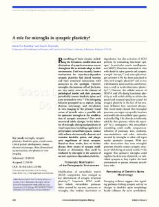
Figure 1. Three implementations of the Hebb rule for synaptic plasticity. The strength of the coupling between cell A and cell B is strengthened when they are both active at the same time. (a) Postsynaptic site for coincidence detection. (b) Presynaptic site for coincidence detection. (c) Interneuron detects coincidence.

98

T. j. Sejnowski and G. Tesauro

the product of the two firing rates. This is in fact quite similar to the recently discovered mechanism of associative LTP that has been studied in rat hippocampus (Brown ef al., 1988; this volume). [Strictly speaking, the plasticity in LTP depends not on the postsynaptic firing rate, but instead on the postsynaptic depolarization. However, in practice these two are usually closely related (Kelso et al., 1986).]Even here, there are many different molecular mechanisms possible. For example, even though it is hard to escape a postsynaptic site for the induction of plasticity, the long-term structural change may well be presynaptic (Dolphin et al., 1982). A second possible implementation scheme for the Hebb rule is shown in Fig. lb. In this circuit there is now a feedback projection from the postsynpatic neuron, which forms an axo-axonic synapse on the projection from A to B. The plasticity mechanism involves presynaptic facilitations: one assumes that the strength of the synapse from A to B is increased in proportion to the product of the presynaptic firing rate times the facilitator firing rate (i.e., the postsynaptic firing rate). This type of mechanism also exists and has been extensively studied in Aplysia (Carew et al., 1983; Kandel et al., 1987; Walters and Byme, 1983). Several authors have pointed out that this circuit is a functionally equivalent way of implementing the Hebb rule (Hawkins and Kandel, 1984; Gelperin et al., 1985; Tesauro, 1986; Hawkins, Chapter 5 this volume). A third scheme for implementing the Hebb rule, one that does not specifically require plasticity in individual synapses, is shown in Fig. lc. In this scheme the modifiable synapse from A to B is replaced by an interneuron, I, with a modifiable threshold for initiation of action potentials. The Hebb rule is satisfied if the threshold of I decreases according to the product of the firing rate in the projection from A times the firing rate in the projection from B. This is quite similar, although not strictly equivalent, to the literal Hebb rule, because the effect of changing the interneuron threshold is not identical to the effect of changing the strength of a direct synaptic connection. A plasticity mechanism similar to the one proposed here has been studied in Hermisseizda (Farley and Alkon, 1985; Alkon, 1987) and in models (Tesauro, 1988). The three methods for implementing the Hebb rule shown in Fig. 1 are by no means exhaustive. There is no doubt that nature is more clever than we are at designing mechanisms for plasticity, especially since we are not aware of most evolutionary constraints. These three circuits can be considered equivalent circuits, since they effectively perform the same function even though they differ in the way that they accomplish it. There also are many ways that each circuit could be instantiated at the cellular and molecular levels. Despite major differences between them, we can nonetheless say that they all implement the Hebb rule. Most synapses in cerebral cortex occur on dendrites where complex spatial interactions are possible. For example, the activation of a synapse

i d

6. The Hebb Rule for Synaptic Plasticity

99

might depolarize the dendrite sufficiently to serve as the postsynaptic signal for modifying an adjacent synap e. Such cooperativity between synapses is a generalization of the Hebb rule in which a section of dendrite is considered the functional unit rather than the entire neuron (Finkel and Edelrnan, 1987). Dendritic compartments with voltage-dependent channels have all the properties needed for nonlinear processing units (Shepherd et nl., 1985).

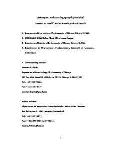
IV. Conditioning The Hebb rule can be used to form associations between one stimulus and another. Such associations can be either static, in which case the resulting neural circuit functions as an associative memory (Steinbuch, 1961; Longuet-Higgins, 1968; Anderson, 1970; Kohonen, 1970), or they can be temporal, in which case the network learns to predict that one stimulus pattern will be followed at a later time by another. The latter case has been extensively studied in classical conditioning experiments, in which repeated temporally paired presentations of a conditioned stimulus (CS) followed by an unconditioned stimulus (US) cause the animal to respond to the CS in a way that is similar to its response to the US. The animal has learned that the presence of the CS predicts the subsequent presence of the US. A simple neural circuit model of the classical conditioning process that uses the Hebb rule is illustrated in Fig. 2. This circuit contains three neurons: a sensory neuron for the CS, a sensorv neuron for the US, and a motor neuron, R, that generates the unconditioned response. There is a strong, unmodifiable synapse from US to R, so that the presence of the US automatically evokes the response. There is also a modifiable synapse from CS to R, which in the naive untrained animal is initially weak. One might think that the straightforward application of the literal interpretation of the Hebb rule, as expressed in Eq. (2), would suffice

Figure 2. Model of classical conditioning using a modified Hebb synapse. The unconditioned stimulus (US) elicits a response in the postsynaptic cell (R). Coincidence of the response with the conditioned stimulus (CS) leads to strengthening of the synapse between CS and R.

100 T. J. Sejnowski and G. Tesauro to generate the desired conditioning effects in the circuit of Fig. 2. However, there are a number of serious problems with this learning algorithm. One of the most serious is the lack of timing sensitivity in Eq. (2). Leaming would occur regardless of the order in which the neurons came to be activated. However, in conditioning we know that the temporal order of stimuli is important-if the US followk the CS, then learning occurs, while if the US appears before the CS, then no learning occurs. Hence Eq. (2) must be modified in some way to include this timing sensitivity. Another serious problem is a sort of "runaway instability" that occurs when the CS-R synapse is strengthened to the point where activity in the CS neuron is able to cause by itself firing of the R neuron. In that case, Eq. (2) would cause the synapse to be strengthened upon presentation of the CS alone, without being followed by the US. However, in real animals we know that presentation of CS alone causes a learned association to be extinguished; that is, the synaptic strength should decrease, not increase. The basic problem is that algorithm 2 is only capable of generating positive learning, and has no way to generate zero or negative learning. It is clear then that the literal Hebb rule needs to be modified to produce desired conditioning phenomena (Tesauro, 1986). One of the most popular ways to overcome the problems of the literal Hebb rule is by using algorithms such as the following (Klopf, 1982; Sutton and Barto,

Here 7, represents the stimulus trace of V , ,that is, the weighted average of V, over previous times, and V , represents the time derivative of V, . The stimulus trace provides the required timing sensitivity so that learning only occurs in forward conditioning and not in backward conditioning. he use of the time derivative of the postsynaptic firing rate, rather than the postsynaptic firing rate, is a way of changing the sign of learning and thus avoiding the runaway instability problem. With this algorithm, extinction would occur because upon onset of the CS, no positive learning takes place due to the presynaptic trace, and negative learning takes place upon offset of the CS. There are many other variations and elaborations of Eq. (3), which behave in a slightly different way, and which take into account other conditioning behaviors such as second-order conditioning and blocking, and for the details we refer the reader to Sutton and Barto (1981), Sutton (1987), Klopf (1988), Gluck and Thompson (1987), Tesauro (1986), and Gelperin et al. (1985); see also Chapters 4, 5, 7, 9, 11, this volume. However, all of these other algorithms are built upon the same basic notion of modifying the literal Hebb rule to incorporate a mechanism of timing sensitivity and a mechanism for changing the sign of learning.

I

I

.

1

6 . The Hebb Rule for Synaptic Plasticity

101

V. Conclusions The algorithmic level is a fruitful one for pursuing network models at the present time for two reasons. First, working top-down from computational considerations is difficult since our intuitions about the computational level in the brain may be wrong or misleading. Knowing more about the computational capabilities of simple neural networks may help us gain a better intuition. Second, working from the bottom up can be treacherous, since we may not yet know the relevant signals in the nervous system that support information processing. The study of learning in model networks can help guide the search for neural mechanisms underlying learning and memory. Thus, network models at the algorithmic level are a unifying framework within which to explore neural information processing. Hebb's learning rule has led to a fruitful line of experimental research and a rich set of network models. The Hebb synapse is a building block for many different neural network algorithms. As experiments refine the parameters for Hebbian plasticity in particular brain areas, it should become possible to begin refining network models for those areas. There is still a formidable gap between the complexity of real brain circuits and the simplicity of the current generation of network models. As models and experiments evolve the common bonds linking them are likely to be postulates like the Hebb synapse, which serve as algorithmic building blocks. It is curious that the Golgi studies of Lorente de N6 should have led Hebb to suggest dynamic rules for synaptic plasticity and dynamic processing in neural assemblies. Ramon y Cajal, too, was inspired by static images of neurons to postulate many dynamical principles, such as the polarization of information flow in neurons and the pathfinding of growth cones during development. This suggests that structure in the brain may continue to be a source of inspiration for more algorithmic building blocks, if we could only see as clearly as Cajal and Hebb.

References Alkon, D. L. (1987). "Memory Traces in the Brain." Oxford Univ. Press, London and New York. Anderson, J. A. (1970). Two models for memory organization using interacting traces. Math. Biosci. 8, 137-160. Artola, A., and Singer, W. (1987). Long-term potentiation and NMDA receptors in rat visual cortex. Nature 330, 649-652. Brown, T. H., Chang, V. C., Ganong, A. H., and Keenan, C . L., Kelso, 5. R., (1988). Biophysical properties of dendrites and spines that may control the induction and expression of long-term synaptic potentiation. In "Long-Term Potentiation: From Biophysics to Behavior" (P. W. Landfield and S. A. Deadwyler, eds.) pp. 201-264. Alan R. Liss, Inc., New York.

102

T. J. Sejnowski and C. Tesauro

Carew, T. J. Hawkins, R. D., and Kandel, E. R. (1983). Differential classical conditioning of a defensive withdrawal reflex in Aplusia caiifornica. Science 219, 397400. Churchland. P. S., and Sejnowski, T. J. (1988). Neural representations and neural computations. in "Neural Connections and Mental Computation" (L. Nadel, ed.). MIT Press, Cambridge, Massachusetts. Dolphin, A. C., Errington, M. L., and Bliss, T. V. P. (1982). Long-term potentiation of perforant path in vivo is associated with increased glutamate release. Nntrtre (London) 297, 496. Farley, J., and Alkon, D. L. (1985). Cellular mechanisms of learning, memory and information storage. Annu. Rev. Psychoi. 36, 419-494. Finkel, L. H., and Edelman, G. M. (1987). Population rules for synapses in networks. i n "Synaptic Function" (G. M. Edelman, W. E. Gall, and W. M. Cowan, eds.), pp. 711757. Wiley, New York. Gelperin, A., Hopfield, J. J., and Tank, D. W. (1985). The logic of Limax learning. 111 "Model Neural Networks and Behavior" (A. I. Selverston, ed.), 237-261. Plenum, New York. Gluck, M. A., and Thompson, R. F. (1987). Modeling the neural substrates of associative learning and memory: A computational approach. Psychol. Rev. 94, 176-191. Hawkins, R. D., and Kandel, E. R. (1984). Is there a cell-biological alphabet for simple forms of learning? Psychol. Rev. 91, 375-391. Hebb, D. 0 . (1949). "The Organization of Behavior." Wiley, New York. Hopfield, J. J., and Tank, D. W. (1986). Computing with neural circuits: A model. Science 233, 625-633. Kandel, E. R., Klein, M., Hochner, B., Shuster, M., Siegelbaum, S. A., Hawkins, R. D., Glanzman, D. L., and Castellucci, V. F. (1987). Synaptic modulation and learning: New insights into synaptic transmission from the study of behavior. In "Synaptic Function" (G. M. Edelman, W. E. Gall, and W. M. Cowan, eds.), pp. 471-518. Wiley, New York. Kelso, S. R., Ganong, A. H., and Brown, T. H. (1986). Hebbian synapses in hippocampus. Proc. Natl. Acad. Sci. U.S.A. 83, 5326-5330. Klopf, A. H. (1982). "The Hedonistic Neuron: A Theory of Memory, Learning, and Intelligence." Hemisphere, New York. Klopf, A. H. (1988). A neuronal model of classical conditioning. Psychobiolog!y 16, 85-125. Kohonen, T. (1970). Correlation matrix memories. 1EEE Trans. Comprrt. C-21, 353-359. Kohonen, T. (1984). "Self-Organization and Associative Memory." Springer-Verlag, Berlin and New York. Komatsu, Y., Fujii, K., Maeda, J., Sakaguchi, H., and Toyama, K. (1988). Long-term potentiation of synaptic transmission in kitten visual cortex. l. Netrroph!ysit~/.59, 124-141. Levv, W. B., Brassel, S. E., and Moore, S. D. (1983). Partial quantification of the associative synaptic learning rule of the dentate gyrus. Neuroscience 8, 799-808. Longuet-Higgins, H. C. (1968). Holographic model of temporal recall. Nntrfre ( L o n d ~ n217, ) 104-107. Marr, D. (1982). "Vision." Freeman, San Francisco, California. McNaughton, B. L., and Morris, R. G. (1987). Hippocampal synaptic enchancement and information storage within a distributed memory system. Trends Nerrrosci. 10,408415. McNaughton, B. L., Douglas, R. M., and Goddard, G. V. (1978). Brain Res. 157, 277. Rumelhart, D. E., and McClelland, J. L., eds. (1986). "Parallel Distributed Processing: Explorations in the Microstructure of Cognition," Vol. 1. MIT Press, Cambridge, Massachusetts. Sejnowski, T. J. (1981). Skeleton filters in the brain. 1n "Parallel Models of Associative Memory" (C. E. Hinton and J. A. Anderson, eds.), pp. 189-212. Erlbaum, Hillsdale, New Jersey. Sejnowski, T. J., and Tesauro, G. (1988). Building network learning algorithms from Hebbian synapses. 111 "Brain Organization and Memory: Cells, Systems and Circuits" (1. L. McGaugh, N. M. Weinberger, and G. Lynch, eds.). Oxtord University Press, New York.

6. The Hebb Rule for Synaptic Plasticity

103

Shepherd, G.M., Brayton, R. K., Millcr, J. P., Segev, I., Rinzel, 1.. and RaI1, W. (1985). Signal enhancement in distal cortical dendrites by means of interactions bctwrcn active dendritic spines. Priu. Notl. Acod. Sci. U.S.A. 82, 2192-2195. Steinbuch, K. (1961). Die lernmatrix. Kuhtrr~etik1, 36-45. Sutton, R. S. (1987). A temporal-difference model of classical conditioning. GTE L n l l . T d r . Rep. TR87-509.2. Sutton, R. S. and Barto, A. G. (1981). Toward a modern theory of adaptive networks: Expectation and prediction. Psyclrol. Rnr. 88, 135-170. Tesauro, G. (1986). Simple neural models of classical conditioning. Bid. Cylwrm~t.55, 187200. Tesauro, G. (1988). A plausible neural circuit for classical conditioning without synaptic plasticity. Proc. Notl. Acnd. Sci. U.S.A. 85, 2830-2833. Walters, E. T., and Byrne, J. H. (1983). Associative conditioning of single sensory neurons suggests a cellular mechanism for learning. Science 219, 405-408. Wigstrom, H.,and Gustafsson, 8. (1985). Acto Physiol. Scoi~d.123, 519.