Michele Mosca∗. Artur Ekert†. May 1998 ...... [BBCDMSSSW] Barenco, A., Bennett, C.H., Cleve, R, DiVincenzo, D.P., Mar- golus, N., Shor, P., Sleater, T., Smolin, ...
arXiv:quant-ph/9903071v1 20 Mar 1999
The Hidden Subgroup Problem and Eigenvalue Estimation on a Quantum Computer Michele Mosca∗
Artur Ekert†
May 1998
Abstract A quantum computer can efficiently find the order of an element in a group, factors of composite integers, discrete logarithms, stabilisers in Abelian groups, and hidden or unknown subgroups of Abelian groups. It is already known how to phrase the first four problems as the estimation of eigenvalues of certain unitary operators. Here we show how the solution to the more general Abelian hidden subgroup problem can also be described and analysed as such. We then point out how certain instances of these problems can be solved with only one control qubit, or flying qubits, instead of entire registers of control qubits.
1
Introduction
Shor’s approach to factoring [Sh], (by finding the order of elements in the multiplicative group of integers mod N , referred to as Z∗N ) is to extract the period in a superposition by applying a Fourier transform. Another approach, based on Kitaev’s technique [Ki], is to estimate an eigenvalue of a certain unitary operator. The difference between the two analyses is that the first one considers (or even ’measures’ or ’observes’) the target or output register in the standard computational basis, while the analysis we detail here considers the target register in a basis containing eigenvectors of unitary operators related to the function f . The actual network of quantum gates, as highlighted in [CEMM], is the same for both algorithms; it is helpful to understand both approaches. In some cases, which we discuss in Sect. 5, this approach suggests implementations which do not require a register of control qubits. A more general formulation of the order-finding problem as well as the discrete logarithm problem, and the Abelian stabiliser problem, is the hidden subgroup problem (or the unknown subgroup problem [Hø]). In the case that G is presented as the product of a finite number of cyclic groups (so G is finitely generated and Abelian), all of these ∗ Clarendon Laboratory, Parks Road, Oxford, OX1 3PU, U.K. and Mathematical Institute, 24-29 St. Giles’, Oxford, OX1 3LB, U.K. † Clarendon Laboratory, Parks Road, Oxford, OX1 3PU, U.K.
1
Figure 1: The function f can be viewed as the composition of a homomorphism g to a group H, and some 1-to-1 mapping h to the set X. Our hidden subgroup K will be the kernel of g, and H is isomorphic to G/K. problems are solved by the familiar sequence of a Fourier transform, a function application, and an inverse Fourier transform. In this paper we describe how this more general problem can also be viewed and analysed as an estimation of eigenvalues of unitary operators.
2
The Hidden Subgroup Problem
Let f be a function from a finitely generated group G to a finite set X such that f is constant on the cosets of a subgroup K (of finite index, since X is finite), and distinct on each coset. The hidden subgroup problem is to find K (that is, a generating set for K), given a way of computing f . When K is normal in G, we could in fact decompose f as h ◦ g, where g is a homomorphism from G to some finite group H, and h is some 1-to-1 mapping from H to the set X. In this case, K corresponds to the kernel of g and H is isomorphic to G/K. We will occasionally refer to this decomposition, which we illustrate in Fig. 1. Define the input size, n, to be of order log2 [G : K]. We will count the number of operations, or the running time, in terms of n. An algorithm is considered efficient if its running time is polynomial in the input size. By elementary quantum operations, we are referring to a finite set of quantum logic gates which allow us to approximate any unitary operation. See [BBCDMSSSW] for a discussion and further references. Our running times will always refer to expected running times, unless explicitly stated otherwise. By expected running
2
time we are referring to the expected number of operations for any input (and not just an average of the expected running times over all inputs). We should be clear about what it means to have a finitely generated group G, and to be able to compute the function f . This is difficult without losing some generality or being dry and technical, or both. The algorithms we describe only apply for groups G which are represented as finite tuples of integers corresponding to the direct product of cyclic groups (consequently, G is finitely generated and Abelian). Conversely, for any finitely generated Abelian G, there is a temptation to point out that G is isomorphic to such a direct product of cyclic groups, and assume that we can easily access this product structure. This is not always the case, even in cases of practical interest. For example, Z∗N , the multiplicative group of integers modulo N for some large integer N , which is Abelian of order φ(N ) (the Euler φ-function) and thus isomorphic to a product of cyclic groups of prime power order. We will not necessarily know φ(N ) or have a factorisation of it along with a set of generators for Z∗N . However, in light of the quantum algorithms described in this paper, we could efficiently find such an isomorphism, thereby increasing the number of finitely generated Abelian groups which can be efficiently expressed in a manner which allows us to employ these algorithms. We will however leave further discussion of these details to another note [EM]. When we talk about computing f , we assume that we have some unitary operation Uf which takes us from state | xi | 0i to | xi | f (x)i. It could, for example, take | xi | yi to | xi | y + f (x)i, where + denotes an appropriate group operation, such as addition modulo N when the second register is used to represent the integers modulo N . Various cases of the hidden subgroup problem are described in [Si], [Sh], [Ki], [BL], [Gr], [Jo], [CEMM], and [Hø]. We note that [BL] also covers the case that f is not necessarily distinct on each coset (that is, h is not 1-to-1), and this is discussed in the appendix. Finding the order r of an element in a group H of unknown size, or the period r of a function f , is a special case where G = Z and K = rZ. For any generator ej of a finitely generated G, we can use the algorithm in Sect. 4.2 to find an integer k such that f (kej ) = f (0), so that kej ∈ K. We find this k with O(n) applications of f and O(n2 ) other elementary quantum operations. We can then assume that ej is of order k (that is, factor hkej i out of G), and in general assume that G is a finite group. We give a few examples. Deutsch’s Problem: Consider a function f mapping Z2 = {0, 1} to {0, 1}. Then f (x) = f (y) if and only if x − y ∈ K, where where K is either {0} or Z2 = {0, 1}. If K is {0}, then f is 1 − to − 1 (or balanced ), and if K is Z2 then f is constant. [De] [CEMM] Simon’s Problem: Consider a function f from Z2 l to some set X with the property that f (x) = f (y) if and only if x − y ∈ {0, s} for some string s of length l. Here K = {0, s} is the hidden subgroup of Z2 l . Simon [Si] presents an efficient algorithm for solving this problem, and the solution to the hidden subgroup problem in the Abelian case is a generalisation.
3
Discrete Logarithms: Let G be the group Zr ×Zr where Zr is the additive group of integers modulo r. Let the set X be the subgroup generated by some element a of a group H, with ar = 1. For example, H = F∗q , the multiplicative group of the field of order q, where r = q − 1. Let a, b ∈ G, and suppose b = am . Define f to map (x, y) to ax by . Here the hidden subgroup of G is K = {(k, −km)|k = 0, 1, . . . , r − 1} = h(1, −m)i, the subgroup generated by (1, −m). Finding this hidden subgroup will give us the logarithm of b to the base a. The security of the U.S. Digital Signature Algorithm is based on the computational difficulty of this problem in F∗q (see [MOV] for details and references). Here the input size is n = ⌈log2 r⌉. Shor’s algorithm [Sh] was the first to solve this problem efficiently. In this case, f is also a homomorphism which can make implementations more simple as described in Sect. 5. Self-Shift-Equivalent Polynomials: Given a polynomial P in l variables X1 , X2 , . . . , Xl over Fq , the function f which maps (a1 , a2 , . . . , al ) ∈ Flq to P (X1 − a1 , X2 − a2 , . . . , Xl − al ) is constant on cosets of a subgroup K of Flq . This subgroup K is the set of self-shift-equivalences of the polynomial P . Grigoriev [Gr] shows how to compute this subgroup. He also shows, in the case that q has characteristic 2, how to decide if two polynomials P1 and P2 are shift-equivalent, and to generate the set of elements (a1 , a2 , . . . , al ) such that P1 (X1 − a1 , X2 − a2 , . . . , Xl − al ) = P2 (X1 , X2 , . . . , Xl ). The input size n is at most l log2 q. Abelian Stabiliser Problem: Let G be any group acting on a finite set X. That is, each element of G acts as a map from X to X, in such a way that for any two elements a, b ∈ G, a(b(x)) = (ab)(x) for all x ∈ X. For a particular element x of X, the set of elements which fix x (that is, the elements a ∈ G such that a(x) = x), form a subgroup. This subgroup is called the stabiliser of x in G, denoted StG (x). Let fx denote the function from G to X which maps g ∈ G to g(x). The hidden subgroup corresponding to fx is K = StG (x). The finitely generated Abelian case of this problem was solved by Kitaev [Ki], and includes finding orders and discrete logarithms as special cases.
3
Phase Estimation and the Quantum Fourier Transform
In this section, we review the relationship between phase estimation and the quantum Fourier transform which was highlighted in [CEMM]. The quantum Fourier transform for the cyclic group of order N , FN , maps N −1 1 X 2πiax/N e | xi . | ai → √ N x=0
4
So FN−1 maps
N −1 1 X 2πiax/N √ e | xi → | ai . N x=0
More generally, for any φ, 0 ≤ φ < 1, FN−1 maps
N −1 N −1 X 1 X 2πiφx √ e | xi → αφ,x | xi N x=0 x=0
(1)
where the amplitudes αφ,x are concentrated near values of x such that x/N are good estimates of φ. The closest estimate of φ will have amplitude at least 4/π 2 . The probability that x/N will be within k/N of φ is at least 1 − 1/(2k − 1). See [CEMM] for details in the case that N is a power of 2; the same proof works for any N . Thus to estimate φ such that, with probability at least 1 − ǫ, the error is less than 1/M , we should use a control register containing values from 0 to N − 1 and apply FN−1 for any N ≥ M (1/ǫ + 1)/2. For example, if we desire an error of at most 1/2n with probability at least 1−1/2m we could use N = 2n+m . In practice, it will be best to use the N that corresponds to the group that is easiest to represent and work with in the particular physical realisation of the quantum computer at hand. We expect that this N will be a power of two. For convenience, we will omit normalising factors in the remainder of this paper. It will also be convenient to have a compact notation for the state on the right hand side of (1) which �to be a good estimator for | φi. So � we consider e let us refer to this state as φ N or just φe if the value of N is understood. Lastly, we will use exp(x) to denote ex .
4
The Algorithm
To restrict attention from finitely generated groups G to finite groups we need to know how to solve the cyclic case (just one generator), that is, to find the period of a function from Z to the set X. We will first describe how to find the order of an element a in a group H, or equivalently, the period of the function f : t → at , as Shor [Sh] did for the group H = Z∗N , the multiplicative group of integers modulo N . We will then show how to generalise it to find the period of any function f : Z → X. If f were a homomorphism (so h is an isomorphism of H, when f is decomposed as f = h ◦ g), we would just be finding the order of f (1) in H. The difference is that we are showing how to deal with a non-trivial h which hides the homomorphism structure. The details will also help explain how to find hidden subgroups of finite Abelian groups.
4.1
Finding Orders in Groups
We have an element a from a group H and we wish to find the smallest positive integer r such that ar = 1. The group H is not necessarily Abelian; all that matters is that the subgroup generated by a is Abelian, and this is always true. 5
The idea is to create an operator Ua which corresponds to multiplication by a (so it maps | yi to | ayi). Since ar = 1, then Uar = I, the identity operator. Hence the eigenvalues of Ua are rth roots of unity, exp(2πik/r), k = 0, 1, . . . , r − 1. By estimating a random eigenvalue of Ua , with accuracy 1/2r2 , we can determine the fraction k/r. The denominator (with the fraction in lowest terms) will be a factor of r. We thus seek to estimate an eigenvalue of Ua ; note that Uar = Uar . For any integer x define Uax to be the operator that maps | yi to | ax yi. Define Uax to be the operator which maps | xi | yi to | xi Uax | yi = | xi | ax yi. Note that Uax acts on two registers and x is a variable which takes on the value in the first register, while Uax acts on one register and x is fixed. Consider the eigenvectors | Ψk i =
r−1 X t=0
� exp(−2πikt/r) at , k = 0, 1, . . . , r − 1,
(2)
of Uax and respective eigenvalues exp(2πikx/r) . If we start with the superposition l 2X −1 | xi | Ψk i x=0
and then apply Uax we get
l 2X −1
x=0
exp(2πikx/r) | xi | Ψk i .
to the first register gives As discussed in the previous section, applying F2−1 l g � | Ψk i and thus a good estimate of k/r. k/r Pr We will not typically have | Ψk i but we do know that | 1i = k=0 | Ψk i. Therefore we can start with r r X X | 0i | 1i = | 0i | Ψk i = | 0i | Ψk i (3) k=0
k=0
and then apply F2l to the first register to produce l r−1 2X −1 X | xi | Ψk i . k=0
We then apply Uax to get r−1 X
k=0
l 2X −1
x=0
(4)
x=0
exp(2πikx/r) | xi | Ψk i
(5)
followed by F2−1 on the control register to yield l r−1 X g � | Ψk i . k/r k=0
6
(6)
Observing the first register will give an estimate of k/r for an integer k chosen uniformly at random from the set {0, 1, . . . , r − 1}. As shown in [Sh], we choose l > 2 log2 r, and use the continued fractions algorithm to find the fraction k/r. Of course, we do not know r, so we must either use an l we know will be larger than 2 log2 r, such as 2 log2 N in the case that H is Z∗N . (Alternatively, we could guess a lower bound for r, and if the algorithm fails, subsequently double the guess and repeat.) We then repeat O(1) times to find r. This algorithm thus uses O(1) exponentiations, or O(n) group multiplications, and O(n2 ) elementary quantum operations to do the Fourier transforms. We can factor the integer N by finding orders of elements in Z∗N . This uses only O(n3 ) or exp(c log n) elementary quantum operations, for c = 3 + o(1) (or c = 2 + o(1) if we use fast Fourier transform techniques). Other deterministic √ factoring methods will factor N in O( N ) or exp(cn) steps, where c = 1/2 + o(1). The best known rigorous probabilistic classical algorithm (using index calculus methods) [LP] uses exp(c(n log n)1/2 ) elementary classical operations, c = 1 + o(1). There is also an algorithm with a heuristic expected running time of exp(c(n1/3 (log n)2/3 ) elementary classical operations (see [MOV] for an overview and references) for c = 1.902 + o(1). Thus, in terms of elementary operations, a quantum computer provides a drastic improvement over known classical methods to factor integers.
4.2
Finding the Period of a Function
The above algorithm, as pointed out in [BL], can be applied to a more general setting. Replace the mapping from t to at with any function f from the integers to some finite set X. Define Uf (x) to be an operator that maps f (y) to f (y + x). This is a generalisation of Uax except it does not matter how it is defined on values not in the range of f , as long as it is unitary. Define Uf (x) to be an operator which maps | xi | f (y)i to | xi Uf (x) | f (y)i = | xi | f (y + x)i. The following are eigenvectors of Uf (x) : | Ψk i =
r−1 X t=0
exp(−2πikt/r) | f (t)i , k = 0, 1, . . . , r − 1,
(7)
with respective eigenvalues exp(2πikx/r). As in (3), we can start with | 0i | f (0)i =
r−1 X
k=0
| 0i | Ψk i
except with our new, more general, definition of | Ψk i. We apply F2n to the first register to produce (4), and then apply Uf (x) to produce (5), followed by F2−1 n to get (6). Observing the first register will give an estimate of k/r for an integer k chosen uniformly at random, and the same analysis as in the previous section applies to find r. One important issue is how to compute Uf (x) only knowing how to compute f . Note that from (4) to (5) (using the modified definition of | Ψk i) we simply 7
go from n 2X −1
x=0
to
n 2X −1
x=0
| xi | f (0)i =
| xi | f (x)i =
n 2X −1
x=0
n 2X −1
x=0
| xi
r−1 X k=0
r−1 X
k=0
!
| xi | Ψk i
(8) !
exp(2πixk/r) | Ψk i
(9)
which could be accomplished by applying Uf , which we do have, to the starting state n 2X −1 | xi | 0i . x=0
Thus even if we do not know how to explicitly compute the operators Uf (x) , any operator Uf which computes the function f will give us the state (9). This state permits us to estimate an eigenvalue of Uf (x) which lets us find the period of the function f with just O(1) applications of the operator Uf and O(n2 ) other elementary operations. The equality in (9) is the key to the equivalence between the two approaches to these quantum algorithms. On the left hand side is the original approach ([Si], [Sh], [BL]) which considers the target register in the standard computational basis. We can analyse the Fourier transform of the preimages of these basis states, which is less easy when the Fourier transforms do not exactly correspond to the group G. On the right hand side of (9) we consider the target register in a basis containing the eigenvectors of the unitary operators which we apply to it (as done in [Ki] and [CEMM], for example), and this gives us (5), from which it is easy to see and analyse the effect of the inverse Fourier transform even when it does not perfectly match the size of G.
4.3
Finding Hidden Subgroups
As discussed in Sect. 2, any finite Abelian group G is the product of cyclic groups. In light of the order-finding algorithm, which also permits us to factor, we can assume that the group G is represented as a product of cyclic groups of prime power order. Further, for any product of two groups Gp and Gq whose orders are coprime, any subgroup K of Gp × Gq must be equal to Kp × Kq from some subgroups Kp and Kq of Gp and Gq respectively. We can therefore consider our function f separately on Gp and Gq and determine Kp and Kq separately. Thus we can further restrict ourselves to groups G of prime power order. This not only simplifies any analysis, it could reduce the size of quantum control registers necessary in any implementation of these algorithms. Let us thus assume that G = Zpm1 × Zpm2 × · · · × Zpml for some prime p and positive integers m1 ≤ m2 ≤ · · · ≤ ml = m. The ‘promise’ is that f is constant on cosets of a subgroup K, and distinct on each coset. The hidden subgroup K is {k = (k1 , k2 , . . . , kl )|f (x) = f (x + k) for all x ∈ G}. In practice, this will usually be a consequence of the nature of f , as in the case of discrete logarithms where f (x1 , x2 ) = ax1 bx2 , or whenever f is constructed as h ◦ g for 8
some homomorphism g from G to some finite group H, and a 1-to-1 mapping h from H to the set X. Let Uf be an operator which maps | xi | 0i to | xi | f (x)i. Define e1 = (1, 0, . . . , 0), e2 = (0, 1, 0, . . . , 0), and so on. Let us also consider an operator related to Uf , Uf (xej ) , which maps | xi | f (y)i to | xi Uf (xej ) | f (y)i = | xi | f (y + xej )i. In the case of Simon’s Problem, the operator Uf (x(0,1,0)) maps | 1i | f (y1 , y2 , y3 )i to | 1i Uf (0,1,0) | f (y1 , y2 , y3 ))i = | 1i | f (y1 , y2 + 1, y3 )i and does nothing to | 0i | f (y1 , y2 , y3 )i. For each t = (t1 , t2 , . . . , tl ), 0 ≤ tj < pmj , satisfying l X j=1
pm−mj hj tj = 0 mod pm for all h ∈ K
define | Ψt i =
X
a∈G/K
exp
l −2πi X
pm
j=1
pm−mj tj aj | f (a)i .
(10)
(11)
We are summing over a set of representatives of the cosets of K modulo G, and by condition (10) on t, this sum is well-defined. Let T denote the set of t satisfying (10), which corresponds to the group of characters of G/K. The | Ψt i are eigenvectors of each Uf (xej ) , with respective eigenvalues exp(2πixtj /pmj ) . By determining these eigenvalues, for j = 1, 2, . . . , l, we will determine t. If we had | Ψt i in an auxiliary register, we could estimate tj /pmj using Uf (xej ) by the technique of the previous section. If we use Fp−1 mj we would determine tj exactly, −1 or we could use the simpler F2k , for some k > log2 (pmj ), and obtain tj with −1 high probability. For simplicity, we will use Fp−1 mj . In practice we could use F k 2 for a large enough k so that the probability of error is sufficiently small. By estimating tj /pmj for j = 1, 2, . . . , l, we determine t. The algorithm starts by preparing l control registers in the state | 0i and one target or auxiliary register in the state | Ψt i, applies the appropriate Fourier transforms to produce 1 pm X−1
x1 =0
!
l −1 pm X
| x1 i · · ·
xl =0
!
| xl i | Ψt i
(12)
followed by Uf (xej ) for j = 1, 2, . . . , n, using the jth register as the control and | Ψt i as the target, to produce 1 −1 pm X
x1 =0
! x1 t1 exp(2πi m1 ) | x1 i · · · p
l −1 pm X
xl =0
! xl tl exp(2πi m ) | xl i | Ψt i . p l
(13)
Then apply Fp−1 mj to the jth control register for each j to yield | t1 i | t2 i . . . | tl i | Ψ t i
9
(14)
from which we can extract t. As in the previous section, we do not know how to construct | Ψt i, but we do know that X | f (0)i = | Ψt i . t∈T
So we start with | 0i | 0i · · · | 0i | f (0)i =
X
t∈T
| 0i | 0i · · · | 0i | Ψt i
apply Fourier transforms to get X
t∈T
1 pm X−1
x1 =0
!
l −1 pm X
| x1 i · · ·
xl =0
!
| xl i | Ψt i
(15)
then apply Uf (xej ) using the jth register as a control register, for j = 1, 2, . . . , n, and the last register as the target register to produce X
t∈T
1 −1 pm X
x1 =0
! x1 t1 exp(2πi m1 ) | x1 i · · · p
l −1 pm X
xl =0
! xl tl exp(2πi m ) | xl i | Ψt i . p l
(16)
We finally apply Fp−1 mj to the jth control register for j = 1, 2, . . . , l, to produce X
t∈T
| ti | Ψt i .
(17)
Observing the first register lets us sample the t’s uniformly at random, and thus with O(n) repetitions we will, by (10), have enough independent linear relations for us to determine a generating set K. For example, in the case of Pfor l Simon’s problem, the | ti all satisfy t · s = j=1 tj sj mod 2 = 0 mod 2, where K = {0, s}. We could also guarantee that each new non-zero element of T will increase the span by a technique discussed in the appendix. This analysis of eigenvectors and eigenvalues is based on the work in [Ki]. The problem is that, unlike in [Ki], we do not always have the operator Uf (xej ) . However, note that, like in Sect. 4.2, going from (15) to (16) maps X | xi | f (0)i 0≤xj ≤pmj
to
X
mj
0≤xj ≤p
=
X
t∈T
1 −1 pm X
x1 =0
| xi | f (x)i
! x1 t1 exp(2πi m1 ) | x1 i · · · p 10
l −1 pm X
xl =0
! xl tl exp(2πi m ) | xl i | Ψt i . p l
We can create state (16) by applying Uf , which we do have, to the starting state X | xi | 0i 0≤xi 1. A similar technique will reduce G = Zpl1 × · · · Zplk to a quotient group G and we can again proceed inductively until the size of G is less than m2 . We can then exhaustively test G for the hidden subgroup K in another O(m2 ) steps. We emphasize that this is a worst-case analysis. If there were a noticeable difference in the behaviour of a 1-to-1 and an m-to-1 function f , m > 1, we could decide if a given function h is 1-to-1 or many-to-one (by composing h with a function f whose period or hidden Abelian subgroup we know, and test for this difference in behaviour). Distinguishing 1-to-1 functions from many-to-1 functions seems like a very difficult task in general, and would solve the graph automorphism problem, for example.
16