The Home Model for Load Balancing in a Computing Cluster

The Home Model for Load Balancing in a Computing Cluster Aharon Ron Lavi A thesis submitted in partial ful llment of the requirements for the degree of Master of Science Supervised by Prof. Amnon Barak October, 1999

Institute of Computer Science The Hebrew University of Jerusalem Jerusalem 91904, Israel

Acknowledgments I wish to thank my advisor, Prof. Amnon Barak. His advice and help always came in the right moment. Thanks also to Dr. Arie Keren for introducing me to the load balancing framework and helping in the rst stages of the thesis, to Prof. Yossi Azar for fruitfull discussions about the theory, to Amnon Shiloh for helping me understand (some) kernel mechanisms, and to Raanan Chermoni for his excellent technical assistance. This research was supported in part by grants from the Ministry of Defense, the Ministry of Science and from Dr. and Mrs. Silverston, Cambridge, the UK.

i

Contents 1 Introduction

1

2 Theoretical Background

5

2.1 On-Line Algorithms and Competitive Analysis . . . . . . . . . . . . . . . . . . . . .

5

2.2 The Load Balancing Problem . . . . . . . . . . . . . . . . . . . . . . . . . . . . . . .

6

2.3 Maximal Load Competitive Algorithms . . . . . . . . . . . . . . . . . . . . . . . . .

7

2.3.1 The Greedy Algorithm . . . . . . . . . . . . . . . . . . . . . . . . . . . . . . .

7

2.3.2 The Marginal Cost Algorithm . . . . . . . . . . . . . . . . . . . . . . . . . . .

7

2.4 Current Load Competitive Algorithms . . . . . . . . . . . . . . . . . . . . . . . . . .

8

2.5 Competitive Algorithms for the Lp Norm . . . . . . . . . . . . . . . . . . . . . . . .

9

2.6 Load Balancing of Multiple Cluster Resources . . . . . . . . . . . . . . . . . . . . . . 10

3 The Performance of Existing Algorithms in a Real System

11

3.1 Evaluation Method . . . . . . . . . . . . . . . . . . . . . . . . . . . . . . . . . . . . . 11 3.2 Performance Results . . . . . . . . . . . . . . . . . . . . . . . . . . . . . . . . . . . . 13 3.3 The MOSIX Policy . . . . . . . . . . . . . . . . . . . . . . . . . . . . . . . . . . . . . 14 3.4 Summary . . . . . . . . . . . . . . . . . . . . . . . . . . . . . . . . . . . . . . . . . . 15 ii

4 On-Line Algorithms for the Home Model

17

4.1 Statement of the Problem . . . . . . . . . . . . . . . . . . . . . . . . . . . . . . . . . 17 4.2 Unit Costs at Home . . . . . . . . . . . . . . . . . . . . . . . . . . . . . . . . . . . . 18 4.2.1 Permanent tasks . . . . . . . . . . . . . . . . . . . . . . . . . . . . . . . . . . 19 4.2.2 Temporary tasks . . . . . . . . . . . . . . . . . . . . . . . . . . . . . . . . . . 21 4.3 Variable Costs At Home . . . . . . . . . . . . . . . . . . . . . . . . . . . . . . . . . . 23 4.4 Related Machines in the Home Model . . . . . . . . . . . . . . . . . . . . . . . . . . 27 4.5 The Greedy algorithm . . . . . . . . . . . . . . . . . . . . . . . . . . . . . . . . . . . 28

5 Performance Evaluation of the On-Line Algorithms in the Home Model

29

5.1 Simulation method . . . . . . . . . . . . . . . . . . . . . . . . . . . . . . . . . . . . . 30 5.2 Heuristic improvements to AssignH . . . . . . . . . . . . . . . . . . . . . . . . . . . 30 5.3 The Maximal Load Performance Measure . . . . . . . . . . . . . . . . . . . . . . . . 32 5.4 The Average Slowdown Performance Measure . . . . . . . . . . . . . . . . . . . . . . 35

6 Extensions of The Home Model in a WAN

39

6.1 The Model . . . . . . . . . . . . . . . . . . . . . . . . . . . . . . . . . . . . . . . . . 39 6.2 Future Work . . . . . . . . . . . . . . . . . . . . . . . . . . . . . . . . . . . . . . . . 41

7 Conclusions

43

Bibliography

44

iii

Chapter 1

Introduction A Computing Cluster (CC) is becoming a popular and powerfull platform for various types of computation. A typical CC is composed of several heterogeneous machines connected by a high speed communication netwrok, thus providing a cost-eective computation platform. In order to achieve good performance on such a platform there is a need to balance the load among the cluster machines. Thus, the load balancing strategy, i.e. the job assignment and reassignment strategy, that is used by the CC, is an important factor that aects its performance. Most implementations of a CC use greedy-based heuristics for job assignments and reassignments. This is in contrast to the theoretical knowledge about the performance of on-line load balancing algorithms. The theoretical eld of load balancing has developed signi cantly in the last decade. Results from this eld indicate that when the cluster is not homogenoeus, e.g. with respect to the machines' speed and the I/O demands of the jobs, then there are better algorithms than greedy. Despite of these results, there has not been many research in order to bridge the gap between theory and practice. One exception is the opportunity cost algorithms that was developed using a theoretical basis [1, 13]. These works developed a theoretical framework for the management of several cluster resources as well as I/O and inter process communication overheads. They have also shown, by means of simulations, that their algorithms outperform greedy-based heuristics in many common cases. 1

This thesis follows a similar approach. We develop a theoretical model to better re ect the architecture of a CC, using the home model. This new model is intended to better re ect a general CC architecture by introducing the assumption that each job is created on a speci c machine, its home machine, and it prefers to be executed on that machine, e.g. because of I/O considerations. The home model is needed due to a large gap between two basic theoretical models: the model in which machines are characterized only by their speeds, called the related machines model, and the most general model which assumes no known characterizations of the machines (but achieving relatively weak results because of that), called the unrelated machines model. The home model is located (roughly speaking) in the \middle", between these two models, i.e. it is more restrictive than the unrelated machines model and less restrictive than the related machines model. We de ne the model and develop several theoretical on-line algorithms for load balancing in this model. Our algorithms achieve better competitive ratios and perform less reassignments than the algorithms for the unrelated machines model and the opportunity cost algorithms, which rely on the algorithms for the unrelated machines model. We also show that the greedy algorithm performs poorly in the home model, from the theoretical point of view. After obtaining theoretical algorithms for the home model, we perform empirical analysis of their performance by means of simulations. Their perfomance is compared to that of the greedy and the opportunity cost algorithms. It is shown that the new algorithms perform consistently better than these two approaches. We show that the main advantage of our algorithms is their improvement of the the main \weak point" of the opportunity cost algorithms. The advantage of the opportunity cost algorithms is realized mainly for jobs with complex characteristics, thus making the cluster architecture seem unrelated. For example, jobs that perform I/O to various machines. In this case it is not possible to assume that the fastest machine in the cluster is the preferred machine for all jobs, since this depends on their I/O requirements. On the other hand, when the environment is closely related, e.g. all the jobs have small I/O overheads, a greedy approach still performs better than the opportunity cost approach. The algorithms we develop for the home model do not suer from this drawback. We show that they are better than the greedy method for 2

related environments and better than the opportunity cost method for unrelated environments. There are many implementations of Computing Clusters, although none of them employes theoretical algorithms. These implementations may be categorized according to their job assignment and reassignment strategy (load balancing method). Job assignment strategies can be either static, dynamic or adaptive (preepmtive). Static strategies use no information about the system state when assigning a new arriving job. For example, PVM, a popular parallel programming environment uses a round-robin method to determine the job's assignment [9]. A dynamic strategy assigns a new job based on the current system state. For example, the GLUNIX operating system [10] supports a remote execution service, assigning a new arriving job to the least loaded machine. An adaptive strategy reassigns jobs transparently during their execution in order to improve their performance. For example, the MOSIX operating system [7] provides a set of kernel enhancements in order to provide a dynamic load balancing mechanism. The diversity of computing cluster implementations shows that, technically, this idea is implementable. An important question, though, remains open: what load balancing algorithms should be used. This question is the main concern of this thesis.

Thesis Outline Chapter 2 provides a background to the theoretical eld of on-line load balancing. It de nes the framework for the problem and details some relevant results. In chapter 3, we describe our implementation of the theoretical algorithms of the opportunity cost approach in a real CC, comparing them to the greedy-based load balancing heuristic. To the best of our knowledge, this is the rst time such theoretical methods are used in a real CC. We rely on this implementation to conclude that integrating such theoretical algorithms in a real-world CC is bene cial, both since it improves performance and since it is relatively easy to implement. In chapter 4 we make another step in this direction, and develop the home model from a theoretical point of view. We present several algorithms and prove their competitive ratios. 3

Chapter 5 provides a performance evaluation of several on-line algorithms in the home model. We rst describe several heuristics to improve the performance of our algorithms from chapter 4. We then compare them to the greedy and to the opportunity cost algorithms, showing that they are consistently better. A possible extension to the home model may be to perform load balancing on a CC connected by a Wide Area Network. In chapetr 6 we discuss the implications of this new direction, and detail future work planned in this subject. Our conclusions and suggestions for future work are given in chapter 7.

4

Chapter 2

Theoretical Background This section presents the theoretical problem of on-line load balancing, which is the main basis for this thesis. We present the problem statement, several known measures for competitiveness and their appropriate algorithms. A comprehensive survey of on-line load-balancing may be found in [5].

2.1 On-Line Algorithms and Competitive Analysis An on-line algorithm must make decisions based only on current and past events, without any knowledge of the future. This is in contrast to an o-line algorithm, which has an a priori, complete knowledge about the input sequence, e.g. a sequence of jobs that arrive over time. A competitive analysis [15] is a common technique for measuring the eectiveness of on-line algorithms, by comparing the performance of an on-line algorithm, for any input sequence, to that of the optimal o-line algorithm. More formally, let ALG(I ) be the performance of an on-line algorithm ALG for an input sequence I , and let OPT (I ) be the performance of the optimal o-line algorithm for the same input sequence. Then algorithm ALG is C -competitive, if for any input sequence I , ALG(I )  C
OPT (I ) + , for some constant . 5

2.2 The Load Balancing Problem The load balancing problem describes a model in which jobs arrive on-line and should be executed in one of the machines of the cluster. The on-line algorithm must assign an arriving job immediately to some machine, thus increasing the machine's load. The most common perfomance measure for this problem is the maximal load among all the machines of the cluster, i.e. the goal of the algorithm is to reduce the maximal load encoutered in the entire execution of all the tasks. More formally, the load-balancing problem is de ned as follows: We are given n machines and a sequence of independent jobs that arrive at arbitrary times. A job j is de ned by its load vector, p(j ) = (p1(j ); p2(j );


; pn(j )), where pi (j ) is the load of job j on machine i. When a job arrives it is assigned immediately to one of the machines, in an on-line manner, thereby increasing the load of this machine by the corresponding value of its load vector. There are three known machine types, de ned by the general form of the jobs' load vector:

 Identical machines: 8i; j : pi(j ) = w(j ), where w(j )  0 is the load of job j . This type corresponds to case in which the cluster machines are all indentical.

 Related machines: 8i; j : pi(j ) = w(j )=vi, where w(j ) is as before and vi  0 is the capacity of machine i. For example, this type can model a cluster with machines of dierent speeds.  Unrelated machines: 8i; j : pi(j ) is arbitrary, non-negative, i.e., the load of a job in one machine is unrelated to its load in any other machine. This type can model a cluster of machines with diverse characteristics, e.g., due to I/O, communication, or SMP architecture constraints. Jobs are classi ed into two types: permanent jobs, which run inde nitely (but still arrive over time); and temporary jobs, with a nite duration, which may be unknown at the job arrival time. It is emphasized that this duration is independent of the speci c assignment of the algorithm (e.g. independent of the machine loads), and thus the duration is the same in the on-line and in the o-line setting. 6

2.3 Maximal Load Competitive Algorithms We describe two algorithms and their competitive ratios with respect to the maximal load.

2.3.1 The Greedy Algorithm Greedy is a popular on-line algorithm for load-balancing. This algorithm assigns a new job to a machine in order to minimize the resulting machine load. For this algorithm it was proved that:

Theorem 2.1 ([11]) For identical machines, the greedy algorithm is 2 ? 1=n competitive. Theorem 2.2 ([2]) For related machines, the greedy algorithm is (log n) competitive. Theorem 2.3 ([2]) For unrelated machines, the greedy algorithm is (n) competitive.

2.3.2 The Marginal Cost Algorithm An algorithm that improves the competitive ratio for unrelated machines, called Assign-U, is presented in [2]. This algorithm de nes a non-linear cost function for an assignment of jobs to machines. A new job is assigned in order to minimize its marginal (added) cost. More formally, let li (j ) be the load of machine i before assigning job j , let pi (j ) be the coordinate i of the demand vector of job j , and let 1 < a < 2 be a constant. The on-line algorithm, ASSIGN-U, computes the marginal cost of the assignment of job j to machine i; i 2 [1; n],

Hi (j ) = al (j)+p (j) ? al (j) ; i

i

i

(2.1)

and chooses the assignment that yields a minimal marginal cost.

Theorem 2.4 ([2]) Algorithm Assign-U is (log n) competitive for unrelated machines and permanent jobs.

In order to maintain an O(log n) competitive ratio for temporary jobs, the Assign-U algorithm was modi ed to allow job reassignments between machines during the execution. Reassignments 7

are performed only when a job is terminated. At such time, the algorithm checks if to reassign some running job j from machine i to machine i0. The following \stability" condition is used:

ah (j)+p (j) ? ah (j)  2(al 0 (j)+p 0 (j) ? al 0 (j)) ; i

i

i

i

i

i

(2.2)

where hi (j ) is the load of machine i, just before j was last assigned to i. If the stability condition is not satis ed by some job j , the algorithm reassigns j to a machine i0 that minimizes Hi0 (j ).

Theorem 2.5 ([4]) Algorithm Assign-U is O(log n) competitive for unrelated machines and temporary jobs. It reassign each job at most O(log n) times.

The Doubling Technique The marginal cost algorithms assume that the maximal load of the optimal o-line algorithm, OPT , is known, and that the values li (j ); pi (j ) (for all i; j ) are scaled down, i.e. divided by OPT . When the value of OPT is unknown, it can be approximated using a doubling technique, as shown in [2]. Brie y, the algorithm works in phases, assuming a dierent value of OPT in each phase. The rst phase assumes a very small OPT , e.g., the minimal possible load of the rst job. The value of OPT is doubled at the beginning of each subsequent phase. Within a phase, the algorithm assigns the arriving jobs, ignoring the jobs that were assigned in the previous phases. A new phase is started when a job j arrives and can not be assigned to any machine without causing its resulting load to exceed C
OPT , where C is the exact competitive ratio of the algorithm. This technique increases the competitive ratio by a factor of 4 [2].

2.4 Current Load Competitive Algorithms Algorithms that are competitive with respect to the maximal (peak) load, does not guarantee a \continuous eort" to balance the machine loads, but only an eort to lower the highest, peak load. For example, consider n identical machines and the following scenario. First, n2 unit-load jobs arrive, thus after assigning them, some machine i has load at least n. Now, all the jobs, except the ones assigned to machine i, depart. A maximal load competitive algorithm may leave these 8

jobs assigned to machine i, even if they will continue to run for a long period, since it does not consider the current load of the optimal o-line algorithm. A current load competitive algorithm, on the other hand, will spread the load on all the machines, by reassigning the jobs. Westbrook [16] gives a general method to convert maximal load competitiveness to current load competitiveness for algorithms which use an estimation, , of the o-line maximal load, OPT . Instead of using the doubling technique described earlier, the algorithm maintains several levels, one for each value of . The assignment of jobs to machine is managed by each level independently, using the original algorithm. When a job arrives, it is inserted to the lowest possible level. The same condition that is used for doubling  is used to indicate the success of failure of the insertion. When a j job departs, the algorithm checks if there are running jobs that are assigned to a higher level than the one of job j . If so, it checks if it can reassign one or more of them to lower levels, repeating this process until no more jobs can step down. In order to bound the number of reassignments made, the notion of restart cost is used. Every job j has an associated restart cost, which is the cost of (re)starting its execution on a machine. It is assumed that the restart cost rj of a job j is proportional to its load, i.e. rj = c
pj for a xed P constant c. If we de ne S = j rj , then any algorithm must incur a restart cost of at least S due to the initial assignment of all jobs. In [16], several speci c algorithms that are competitive with respect to current load are presented, e.g a 6-competitive algorithm with 3S restart cost for identical machines and an (8 + )competitive algorithm with O(S ) restart cost for related machines.

2.5 Competitive Algorithms for the Lp Norm Another method for better balancing the loads of the cluster is to consider their L2 norm, i.e. P l2, where M is the set of cluster machines. A general O(p)-competitive algorithm with i2M i respect to the Lp norm for unrelated machines is given in [3]. The algorithm de nes the increase 9

in the Lp norm by assigning job j to machine i as: Increase(j ) = (li + pij )p ? lip where li is the load of machine i when job j arrives, and assigns j to the machine with the minimal increase. It is also shown there that any on-line algorithm will have a competitive ratio of at least

(p).

2.6 Load Balancing of Multiple Cluster Resources In the problem of on-line management of multiple resources in a computing cluster, the goal is to minimize the maximal utilization over all the resources, e.g., CPU, Memory, I/O, etc. An opportunity cost algorithm for solving this problem is presented in [1], where it is used to manage the allocation of CPU and memory resources of sequential jobs. An opportunity cost algorithms for communication and I/O operations of parallel and sequential jobs, in order to minimize the inter process communication and I/O overheads as well as the overall utilization of cluster resources, are presented in [13]. These algorithms extend the Assign-U algorithm described above, using the economical principle of marginal cost. The main contribution of these works is to bridge the gap between theory and practice. Although some aspects of the load balancing theoretical framework does not correspond to reality, they show, by means of simulations, that the opportunity cost approach improves the performance of a real computing cluster. In this thesis we show the rst evaluation of the opportunity cost approach in a real computing cluster, implementing the algorithms inside the operating system. Then, we develop a new model, the home model, and several on-line algorithms for this model, in order to address some weak points of the opportunity cost approach.

10

Chapter 3

The Performance of Existing Algorithms in a Real System This chapter presents the performance of three known algorithms, the opportunity cost algorithm (COST-P), the greedy algorithm (GREEDY-P), and the MOSIX [7] load balancing algorithms, in a real computing cluster. The motivation for this is two fold. First, to show how well the opportunity cost algorithms perform in a real system. So far the performance of these algorithms were tested only by simulations [1, 13]. Second, to show the ability of simulations to predict the results trend in real executions (since simulations are also used in this thesis). In addition, the performance results emphasize some weak points of the opportunity cost algorithms, which are part of the motivation for developing algorithms for the home model, as discussed in the next chapter.

3.1 Evaluation Method The execution cluster consists of 6 machines, two Pentium-Pro 200MHz; two Pentium-II 300MHz and two Pentium-II 400MHz, with memory sizes ranging from 64MB to 256MB. The machines where connected by a Fast Ethernet switch. The executions were performed using a modi ed MOSIX for Linux [8] operating system, which supports preemptive process migration. In each execution, we replaced the existing resource sharing policy of MOSIX with the COST-P or the GREEDY-P policies respectively. 11

The implementation of the COST-P algorithm is a straight forward implementation of the COST-IO algorithm, described in [13], which extends the cost function, 2.1, described in Section 2.3.2 to include the I/O cost. After examining several dierent values for the exponential function, we used a = 1:2. The exponential function includes two resources, CPU and memory. The implementation of the GREEDY-P algorithm is based on the greedy algorithm, as described in Section 2.3.1. In order to provide each machine with complete knowledge about the usage of the resources, as required by the two algorithms, we used a modi ed version of the information gathering and dissemination scheme of MOSIX. We note, that due to scaling considerations, this scheme is based on probabilistic information dissemination, with decentralized control, such that each node has a partial knowledge about other nodes in the cluster. Furthermore, since the estimation of the optimal load must be identical in all the machines, we have added this parameter to the information dissemination mechanism as well. We conducted two sets of tests, one for jobs with I/O overhead and the other for jobs with I/O overhead and a large memory consumption. Each test consists of arriving jobs, with inter-arrival and CPU times exponentially distributed with mean 2 and 7 seconds respectively. the tests were repeated 50 times, with dierent sequences of jobs. 4.5 GREEDY-P COST-P

Slowdown

4

3.5

3

2.5

2 0

0.35

0.7 I/O overhead

Figure 3.1: I/O jobs: mean slowdown vs. I/O overhead. 12

1.05

3.2 Performance Results Figure 3.1 presents the execution results of jobs with I/O overhead. In these executions, the I/O overhead is exponentially distributed with mean ranging from 0 to 1.05. From the gure it can be seen that with increased values of I/O overhead, the opportunity cost policy outperforms the greedy policy. For example, for an I/O overhead of 0:7, i.e. for every second of CPU the job waits 0.7 seconds for I/O, the average slowdown of COST-P is about 20% lower than that of GREEDY-P. Note that for pure CPU bound jobs, GREEDY-P is slightly better, i.e. about 9%, than COST-P. This result con rms the results of the simulations presented in [1, 13]. In the second test, we executed sets of jobs with a relatively large memory consumption. In these executions, the I/O overhead was xed at 35% and the memory usage was exponentially distributed with mean ranging from 0 MBytes to 20 MBytes. 25 GREEDY-P COST-P

Slowdown

20

15

10

5

0 0

5

10

15

20

Memory usage (MBytes)

Figure 3.2: I/O and Memory jobs: mean slowdown vs. memory usage. Figure 3.2 presents the results of these executions. From the gure it follows that as long as the mean memory usage of the jobs is less than 10 MBytes, there is less than 10% dierence between the slowdown of COST-P and GREEDY-P. We suspect that for these size, almost always all the running jobs t in the main memory. Thus execution of jobs in this interval corresponds to the results of jobs with only I/O overhead, as shown in Figure 3.1. When the job sizes is greater than 10 MBytes, COST-P consistently outperforms GREEDY-P, by as much as 100%, for jobs with 13

an average size of 20 MBytes or more.

3.3 The MOSIX Policy At this stage, it is interesting to compare the opportunity cost policy to the ne-tuned, heuristic policy of MOSIX. For this set of tests, we executed the same sets of sequential jobs as in the previous section, using the original MOSIX policy. Brie y, the MOSIX resource sharing policy continuously attempts to reduce the CPU load dierences between pairs of machines, by migrating processes from over-loaded machines to less loaded machines. MOSIX also uses a memory ushering algorithm, which migrates processes from machines that has exhausted their main memory to machines that has free memory. Another heuristic performed by MOSIX is that it chooses the best target machine for each migrating process. This decision is based on gathered information by the system, in order to minimizes the expected remaining process run time. For example, MOSIX takes into account the migration time, based on the process size, past CPU time, amount of I/O performed, etc. These heuristics were veri ed by studies of process and system behavior [6, 12]. 4.5 GREEDY-P COST-P MOSIX

Slowdown

4

3.5

3

2.5

2 0

0.35

0.7

1.05

I/O overhead

Figure 3.3: I/O jobs: mean slowdown vs. I/O overhead. Figure 3.3 compares the slowdown for jobs with I/O overhead between the COST-P and the GREEDY-P, previously shown in Figure 3.1, and the MOSIX policy. From the gure it can be 14

15 GREEDY-P COST-P MOSIX

Slowdown

12

9

6

3

0 0

5

10

15

20

Memory usage (MBytes)

Figure 3.4: Memory jobs: mean slowdown vs. memory usage. seen that MOSIX is slightly better than the other two policies, with an average of 6% improvement over COST-P. The slowdown for jobs with I/O overhead and large memory are presented in Figure 3.4. As can be seen from the gure, as long as the average memory size of the jobs is not greater than 10 MBytes, all three policies has near identical performance. For jobs greater than 10 MBytes, GREEDY-P starts excessive paging, while COST-P and MOSIX are still able to t the running jobs in the cluster's memory. When the average job size is increases beyond 15 MBytes, both COST-P and MOSIX start excessive paging, at about the same rate, still signi cantly lower than GREEDY-P. Thus, in this case as well, the performance of MOSIX and COST-P is similar. Although MOSIX performs similarly to the oportunity cost algorithms, the latter has the ability to add more resources to the mechanism without extra eort, since the theoretical framework supports that. Adding another resource to the MOSIX heuristics is much more dicult, since much tuning has to be done to determine its eect on the previous heuristics employed.

3.4 Summary Since the opportunity cost approach is aimed to function in the most general model of unrelated machines, its competitive ratio is relatively high, and it does not function well if the environment 15

tends to be less unrelated, as demonstrated here by lowering the I/O overhead. In addition, the MOSIX heuristics has similar performance. These are motivations for developing another theoretical model, the home model, which is more related to the structure of CC's in general, and speci cally, to a MOSIX-based CC. In the next chapter, this model is de ned and several on line algorithms are developed. We conclude this chapter by pointing-out that MOSIX converts all migration decisions into time units, assuming a past-repeat estimate on the expected remaining execution time of the job. We note that this assumption was veri ed empirically in [12]. This method enables MOSIX to include in its considerations variables that can only be expressed in time units, e.g., migration cost, network latency, etc. The load-balancing theory, on the other hand, does not deal with such time-dependent variables.

16

Chapter 4

On-Line Algorithms for the Home Model This chapter decribes on-line algorithms for load balancing in the home model, which is a special case of the general on-line load balancing problem. First, we de ne the home model. Then, we give two algorithms for dierent variants of the problem and prove their competitive ratios. We also show that the greedy method performs poorly in this model.

4.1 Statement of the Problem A machine model determines a speci c form for the cost vector, e.g. in the identical machines model all coordinates of the cost vector are identical. There are several machine models known in the literature, as described in chapter 2. We de ne a new machine model, called the home model, in which each task has a \home" machine which it prefers to be assigned to. This is motivated by several realistic cluster architectures. For example, consider a computing cluster composed of several computing centers connected by a Wide Area Network. Each task is generated in one of the computing centers and may be executed in a remote computing center in order to reduce the local load by using remote resources. Each task, though, performs most of its I/O with its originating center and therefore prefers to be assigned there. Another example is the architecture of the MOSIX distributed operating system [7], in which 17

the home machine of a process is the machine it was created on. If a process is migrated to another machine it communicates with the system and with other processes through its home. In this case, if the cluster machines are connected by a LAN, the load the process creates in its home is lower than the load it creates on other machines, since the I/O overhead is due to the CPU processing of the network protocols [13]. More formally, the cost vector of tasks in the home model is de ned as follows:

8 < pj (i) = : p inj i = hj p outj otherwise;

such that 8j : p inj < p outj . The only currently known algorithms for this problem are algorithms for the more general model of unrelated machines. These algorithms have logarithmic competitive ratio, as described in chapter 2. In the following sections we give on-line algorithms for two variants of the home model, unit and variable costs at home, with constant competitive ratios. For this purpose, we extend techniques of Azar et al. [2] regarding load balancing for related machines. We also show that the natural greedy algorithm is (n) competitive in the home model with unit costs, as in the unrelated machines case. In order to reduce the competitive ratio we use a limited number of task reassignments, i.e. moving a task from one machine to another after it has started to execute. We note that experience with real systems shows that task reassignments may be performed with very little overhead, thus achieving a powerfull tool for load balancing [7, 8]. Task reassignments are also used for temporary tasks on unrelated machines [4].

4.2 Unit Costs at Home In this section we consider a variant of the home model in which the cost vector is of the following form: 8 < 8i; 1  i  m : pj (i) = : 1 i = hj pj otherwise ; 18

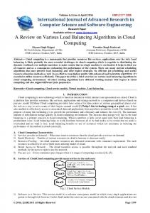
AssignH(j , p~j , ~l, ) (1) if ( lh < 2 ) then lh l h + 1 return(~l, \success") (2) else if (( Out = fj1jj1 2 Jh ; pj1 (hj ) > 1 g 6= ; ) then j out some j1 2 Out such that 8j2 2 Out : pj1 (hj )  pj2 (hj ) (3) else j out j1 2 Jh [ fj g such that 8j2 2 Jh [ fj g : pj1  pj2 (4) if ( 9i : li + pj out (i)  2 ) then li li + pj out (i) if ( j out 6= j ) lh lh ? pj out (i) + 1 return(~l, \success") else return(~l, \fail") j

j

j

j

j

j

j

j

Figure 4.1: The AssignH algorithm such that 8j : pj > 1. Machine hj is the home machine of task j . We rst examine the case of permanent tasks (i.e. tasks that never nish), and then extend the algorithm to the case of temporary tasks.

4.2.1 Permanent tasks Figure 4.1 presents the assignH algorithm for the case of permanent tasks. Its general idea is to assign a new arriving process to its home, if its not too loaded (step 1). Otherwise, it migrates a non-local process from this home (if any), or a less heavier local process (if any), or the new process itself (steps 2 and 3) to a remote machine that is not too overloaded (step 4)). If there is no such machine the algorithm fails. The algorithm determines if a machine is oveloaded using an estimation of the optimal load, . 19

Lemma 4.1 For the set of tasks that assignH assigns outside their homes there is an optimal assignment that assigns all these tasks outside their homes as well, assuming that   OPT ( the value of the optimal assignment).

Assume that there is no such optimal assignment. Let j out be the rst task that assignH assigns to machine i 6= hj out and that in all the optimal assignments j out is assigned to its home. When j out was assigned to machine i it holds that 8j1 2 Jh : pj1 (hj out ) = 1 as a result of step 2 in assignH (otherwise a non-local task would have been reassigned), and that lh  2 > OPT as a result of step 1. Therefore the optimal assignment could not have to hj out (since it assigned j out to hj out ). Let j in 2 Jh be assigned all the tasks j 2 Jh some task that the optimal assignment assigned to machine i1 6= hj out . Since pj in (i1)  pj out (i1) (as a result of step 3), the assignment that would result from swapping j in and j out in the optimal assignment is optimal as well, and j out is assigned outside its home, which is a contradiction. Proof:

j out

j out

j out

j out

Lemma 4.2 If   OPT then assignH never returns \fail". Assume that assignH returns \fail" when trying to assign job j out and that   OPT . Denote by assignOPT the optimal assignment that exists according to Lemma 4.1. Since assignOPT assigned j out outside its home, then pj out (i) = pj out  OPT  . As a result of step 4 (since assignH failed) 8i : li + pj out (i) > 2, and thus: Proof:

li > 2 ? pj out (i)    OPT :

(4.1)

Denote by In; Out the set of tasks that assignH assigned in,outside their homes, respectively. The general notation of X  is used to denote assignOPT's equivalent group to the group X of assignH (e.g. In denotes the set of tasks that assignOPT assigned to their homes). Note that according to Lemma 4.1, Out  Out , and that 8i : li > OPT  li, as shown in equation 4.1. Therefore, it exists that:

X

j 2Out

pj +

X

j 2In

1=

X i

li >

X i

20

li =

X

j 2Out

pj +

X

j 2In

1;

as both left and right equalities derive from the fact that the summation is over all tasks, but the summation order is dierent. From this it follows, that since Out [ In = Out [ In and 8j : pj > 1 there must be some j 2 Out such that j 2= Out , which is a contradiction.

Lemma 4.3 AssignH reassigns a single task no more than m times. We will refer to task j1 as heavier than task j2 if pj1 > pj2 . Assume AssignH reassigned a speci c task j more than m times. Therefore there exists a machine i that j was assigned to at least twice, thus j was reassigned from i to i1 at some time t1 between the two reassignments to i. If i = hj than li = 2 from this point on so j could not have been reassigned back to i and it is a contradiction. Therfore, i 6= hj , and at t1 it exists that li = 2 ? pj + 1. Assume j1 is the rst task that is heavier than j (and i 6= hj1 ) that was assigned to i after t1 , at time t2 (if there is no such job we set j1 = j ). It follows that at time t2 : li + pj1  2 and at time t1 : li + pj1  2 + 1 and therefore there is a task j2 that is heavier than j1 and was reassigned from i at some time between t1 and t2. j2 could not have been assigned to i after t1 since j1 is the rst such task, and could not have been assigned to i before t1 since at that time j was the heaviest task assigned to i, and the contradiction follows.

Proof:

It is easy to verify that assignH never creates load that exceeds 2, and that assignH performs at most one reassignmnet whenever a new task arrives, thus performing no more the n reassignments during the entire running time (i.e. each job is reassigned once, in average over all jobs). In order to estimate the optimal load, we use the doubling technique described in section 2.3.2, which multiply the competitive ratio by 4. Thus we conclude:

Theorem 4.1 Algorithm AssignH is 8 competitive with respect to load, performs at most n reassignments in the entire running time, and reassigns a single task no more than m times.

4.2.2 Temporary tasks We extend the assignH algorithm to handle temporary tasks with unknown durations as well. In this case, each task j has a duration dj , which is unknown to the on-line algorithm until the task 21

AssignHremove(j , ~l) /* Denote by m(j ) the machine that task j is assigned to */ lm(j) lm(j) ? pj (m(j )) if ( m(j ) = hj ) then Outsiders = fj1jhj1 = m(j ) ; m(j1) 6= hj1 g if ( Outsiders 6= ; ) then j in j1 2 Outsiders such that 8j2 2 Outsiders : pj1  pj2 reassign j in to its home return(~l) Figure 4.2: The remove method nishes. As described in chapter 2, the task duration is xed, independent of the load of the machine the task was assigned to (thus the two sets of running tasks, of the o-line and of (any) on-line algorithm are identical). The assignH algorithm is modi ed to include a method for task departures. This method, which is described in gure 4.2, reassigns back home the heaviest task that is assigned outside. Task insertions are handled as before. We get:

Theorem 4.2 Algorithm AssignH for temporary tasks is 8 competitive with respect to load and performs at most 2n reassignments in the entire running time.

We rst show that Lemma 4.1 still holds, when referring to the currently active set of tasks. We prove this by induction on the sequence of job arrivals and departure. If a new job j arrives, the original proof still holds and it remains that Out  Out after reassigning j . If an existing job departs recall that assignH reassigns back home the heaviest job that is assigned outside. Note that only one job may be reassigned back home. If OPT did not perform any reassignment it holds that Out  Out . If it reassigned a dierent job j1, assume by contradiction that no optimal assignment reassigns back the heaviest job, switch between j and j1 and receive such optimal assignment, which is a contradiction (as in the proof of Lemma 4.1). Proof:

Lemma 4.2 still holds, since it relies only on Lemma 4.1 and on the set of active tasks, thus 22

assignH never fails. Since every task arrival and every task departure may cause at most one task reassignment, the algorithm performs at most 2n task reassignments.

4.3 Variable Costs At Home We examine a dierent version of the \home" model, which diers from the previous one by the jobs' cost vector form, de ned by

8< p i = hj pj (i) = : j x  pj otherwise ;

for some (globally) xed constant x > 1. As in the previous model, the algorithm we provide here follows the principle that the sum of weights of \outside tasks" (tasks that are assigned outside their homes) is minimized while keeping the machines not too oveloaded. Since the home costs are dierent, it is not possible to simply replace a task with a heavier one, and thus this operation is less straight-forward in this model. Figure 4.3 details the task insertion operation (as before, it can be viewed as an algorithm for permanent tasks). The algorithm tries to assign each task to its home, even by reassigning strangers (steps 1 and 2). Otherwise it moves out the lightest tasks, if there are enough such tasks, or moves out the new task (steps 3 and 4). The proof of correctness has essentially the same structure as in the previous section. We rst prove correctness for permanent tasks.

Lemma 4.4 De ne Out; Out as the set of tasks that were assigned outside their homes by assignHv and the optimal o-line algorithm, respectively. If   OPT , then: X X pj  pj : j 2Out

j 2Out

We refer to the sum of costs of any group of tasks as the weight of the tasks. Examine any arrival of a task j that causes some home task(s) to be reassigned (possibly j itself), i.e. the algorithm reaches at least step 3. Observe that all the tasks assigned to hj after step 2 are local

Proof:

23

AssignHv(j , p~j , ~l, ) (1) if ( lh + pj  2 ) then lh lh + pj return \success" (2) if there are strangers in hj then j out fenough strangers such that there weight  pj , or all the strangersg loop over all tasks in j out reassign current task to a machine 6= hj such that the resulting load  2 if current task can not be reassigned return \fail" if ( lh + pj  2 ) then assign j home and return \success" (3) sort the tasks in hj such that 8i : pi  pi+1 k minfljpl < pj ; Pli=1 pi  pj g or 0 if ( k = 0 ) assign j to machine 6= hj such that its resulting load is  2 if there is such machine return \success" otherwise return \fail" P (4) if ( lh ? ki=1 pi + pj <  ) then k k ? 1 loop i = 1 to k reassign task i to a machine 6= hj such that the resulting load  2 if task i can not be reassigned return \fail" assign j to hj and return \success" j

j

j

j

j

Figure 4.3: The AssignHv algorithm tasks. It exists that lh > OPT , since pj  OPT and lh + pj > 2  2  OPT . Denote by W the weight of all the local tasks already assigned outside by assignHv. Since the weight of all active tasks exceeds OPT by at least W + pj (because the weight of tasks assigned home is greater than OPT), any algorithm that achieves maximum load OPT must have assigned outside tasks of weight at least W + pj . Therefore, if assignHv assigns task j outside the lemma holds. If assignHv assigns P ?1 p < p (otherwise the rst k ? 1 lighter tasks outside the lemma also immediatly holds since ik=1 i j pk would not have been added). If assignHv reassigns task k as well, it exists that the weight of all P active tasks exceeds OPT by at least W + ki=1 pi (as explicitly veri ed in step 4), thus the lemma j

j

24

holds in this case as well.

Lemma 4.5 If assignHv decides to assign task j 0 outside its home and   OPT then x  pj0  OPT Examine any arrival of a task j that causes some home task(s) to be reassigned. De ne In the set of tasks assigned to this home by assignHv. By Lemma 4.4, the optimal assignment (Opt) must assign tasks with weight at least pj outside from the set of tasks In [ fj g. If assignHv assigned task j outside any assignment must assign j or a heavier task outside, since there is no set of lighter tasks with weight  pj (due to step 3). Thus assume that assignHv assigned task j home and tasks 1 : : :k outside. If Opt assigned task j home then it must assign outside all the tasks 1 : : :k, or some of them and a heavier task, thus completing the proof. Otherwise Opt assigned task j outside and 81  i  k; pi < pj ) x  pi < x  pj  OPT .

Proof:

Lemma 4.6 If   OPT then assignHv never fails. We use In; Out and the general notation of X  as used above (speci cally in Lemma 4.2). Assume by contradiction that assignHv fails when trying to assign task j . This implies that all machines have load greater than OPT, due to Lemma 4.5 and because assignHv fails to assign a task to a machine only if the resulting load is greater than 2  OPT . Therefore,

Proof:

x

X

j 2Out

pj +

X

j 2In

pj =

X i

li >

X i

li = x 

X

j 2Out

pj +

X

j 2In

pj ;

as both left and right equalities derive from the fact that the summation is over all tasks, but the summation order is dierent. Since Out [ In = Out [ In it follows that

X

j 2Out

pj >

X

j 2Out

pj ;

which is a contradiction to Lemma 4.4. In order to give an upper bound for the amount of reassignments made by assignHv, we use the measure of restart cost, de ned by Westbrook [16]. As detailed in chapter 2, it is assumed that 25

P

every task j has an associated restart cost rj = c  pj for a xed constant c. If we de ne S = j rj , then every algorithm must incur a restart cost of at least S due to the initial assignment of all tasks.

Lemma 4.7 assignHv incurs at most 3S restart cost. We show that, upon every arrival of a new task j , assignHv reassigns tasks with total weight less than 2pj , and thus incur a reassignment cost less than c2pj = 2rj . Therefore, the total P ?1 p < p , P reassignment cost < S + j 2rj = 3S . Assume assignHv reassings k tasks. Then, ik=1 i j P k otherwise task k would not have been added, and pk < pj , thus i=1 pi < 2pj .

Proof:

Theorem 4.3 The assignHv algorithm is 8-competitive with respect to load and incurs a total reassignment cost of at most 3S .

It is immediate that assignHv never creates a load that exceeds 2. Lemma 4.6 ensures that assignHv never fails if  > OPT . Therefore, by using the standard doubling technique we conclude that assignHv is 8-competitive. Lemma 4.7 ensures that assignHv incurs a total reassignment cost  3S . Proof:

We now describe the method of handling temporary tasks, which is similar to the one described in section 4.2.2. As detailed there, we must add a method that reassigns home some tasks when a home task departs in order to maitain the correctness of Lemma 4.4. Suppose that task j has departed, we then move back home some tasks that are assigned outside, one by one, starting from the heaviest one, verifying that the home load does not exceed 2, until we reasssign at least pj weight back home. Observe that tasks that are heavier than task j can not be reassigned without oveloading the home machine (otherwise they would have been assigned home when they arrived, reassigning outside j and other tasks if necessary). Therefore, the total weight of tasks reassigned is at most 2pj . Thus we conclude:

Theorem 4.4 The assignHv algorithm for temporary tasks is 8-competitive. It incurs a total reassignment cost of at most 5S .

26

4.4 Related Machines in the Home Model The case of related machines is a re nement to the basic model, in which each machine i has a speed si . The home machine is still the preferred machine to be executed on. The cost vector of task j is now of the general form as follows:

8 < p inj i = hj pj (i) = : p outj =si otherwise ; such that 8i; j : p inj < p outj =si . We describe a general method to integrate the previous algorithms for the home model with the already known algorithms for related machines. We maintain two virtual sets of machines. The rst set is related to an algorithm, H, which is a part of the appropriate home algorithm, including only the decision mechanism whether to assign a task to its home, and which tasks should be assigned outside their homes. The second set is related to an appropriate related machines algorithm, R, which assigns the tasks that H decided to move out of their homes, independently of H (not considering the load created by H), but can not assign a task to its home. H may also retrieve a task from R in a case of task departure. Recall that assignH may create a load due to home tasks of no more than OPT , and that assignHv creates an appropriate load of no more than 2  OPT . Also recall that for both algorithms, the set of tasks assigned outside, OUT , is of smaller weight than that of the optimal algorithm, and 8j 2 OUT , either Opt assigned j outside or it assigned a heavier task outside instead, and thus R can assign all tasks in OUT creating a load no more than c  OPT , c is the appropriate competitive ratio. Westbrook [16] describes an appropriate algorithm for temporary tasks with c = 2 +  which incurs O(S ) reassignment cost. We get:

Theorem 4.5 The method described above for relatd machines in the home model produces a (12+ )-competitive algorithm with O(S ) reassignment cost for unit costs, and a (16 + )-competitive algorithm with O(S ) reassignment cost for variable costs. 27

4.5 The Greedy algorithm The intuitive greedy algorithm assigns a new arriving task j to machine i so that the resulting load, li + pj (i), is minimized. As described in chapter 2, this algorithm is 2 competitive for identical machines, (logn) competitive for related machines, and (n) competitive for unrelated machines. It is interesting to examine how \dicult" the home model is by relating the competitiveness of the greedy algorithm to one of these groups. We show that the lower bound of Azar et al. [2] for unrelated machines is suitable for the home model with unit costs. Since the home model is a special case of unrelated machines, their upper bound holds here as well.

Lemma 4.8 The greedy algorithm is (n) competitive in the home model with unit costs. Assume that ties are broken by assigning a task to the machine with the lower index. For every group of 1 : : :n machines, consider the following 0 : : :n ? 1 task arrivals:

Proof:

h0 = 1; p0 = 1 + ; 8j > 0 : hj = j; pj = j + 1j  Recall that the home costs of all jobs are 1. The greedy algorithm assigns task #0 to its home (machine #1), task #1 to machine #2 (since the resulting load in its home, machine #1, is 2 and the resulting load in machine #2 is 1 +  < 2), task #2 to machine #3 (since the resulting load in its home, machine #2, is 1 + (1 + ) and the resulting load in machine #3 is 2 + 21 ), task #3 to machine #4 (since the resulting load in its home, machine #3, is 1 + (2 + 21 ) and the resulting load in machine #4 is 3 + 31 ), and so on. The last task is assigned to machine #n for a resulting load of (n ? 1) + n?1 1  = O(n). A better assignmnet is to assign each task to its home, thus having maximum load of 2. The optimal assignment assigns each task to its home except for task #0 which is assigned to machine #n, thus the optimal load is 1 + .

28

Chapter 5

Performance Evaluation of the On-Line Algorithms in the Home Model The theoretical framework provides a worst case analysis. Thus, it is important to analyze the average case behaviour of the dierent possible on-line load balancing algorthims in the home model. This chapter presents an empirical analysis of the performance of several algortihms in the home model, based on realistic scenarios, by means of simulations. We analyze the performance using two performance measures. The rst, the maximal load performance measure, corresponds to the theoretical analysis. The second, the average slowdown performance measure, represents another way to measure the eciency of the computing cluster. The slowdown of a job is the relation between its actuall running time and its running time on an idle machine. Although there is no theoretical guarantee about the performance of any of the algorithms with respect to this measure, it is interesting to examine it since it represents some aspect of the CC's performance. Before the performance results are presented, several possible heuristics to improve the performance of the assignH algorithm are suggested and evaluated.

29

5.1 Simulation method In order to simulate the execution of a stream of jobs in a computing cluster, we developed a simulator for this environment. The simulator assigns jobs to machines by a seperate module, which may implement any algorithm, and calculates the allocation of the CPU time of a machine to the jobs assigned to it in another independent module, assuming a time-sharing environment. The scenario for each execution is created randomly, by some distribution function. This includes both the cluster characteristics (e.g. machine speeds) and job characteristics (e.g. amount of CPU time, communication overhead, home machine, etc.). The machines speeds are uniformly distributed between 1 and 2. The jobs' total required CPU time and arrival time are exponentially distributed with mean 2n and 8=n, repectively, where n is the cluster size. The theoretical assumption of xed duration of a job (i.e. the time frame it is running is xed, though unknown, regardless of the load and other variables) is replaced with the more realistic assumption of xed work (i.e. a job runs until it receives the total amount of CPU time it needs). It is assumed that the cluster machines are connected by a Loacl Area Network. Therefore, the network latency is negligible, and thus the communication overhead is translated into CPU overhead (i.e. the latency is due to CPU processing overhead of the various network protocols). All the simulation results presented in this chapter are averaged over 100 executions, and are normalized with respect to the appropriate value achieved by some of the examined methods, making the comparison easier.

5.2 Heuristic improvements to AssignH We consider several heuristics as an addition to the algorithms described in the previous chapter. In this section, the performance improvement of these heuristics is evaluated. One \weak point" of AssignH is the method of evaluating the o-line maximal load, . Recall that the original estimation method is to double  whenever the algorithm fails to assign an 30

arriving job. After such an increase, the algorithm ignores previous jobs and their loads. A possible heuristic addition is to perform a more gradual increase of . Another heuristic is to (still) consider all previously arrived jobs after an increase of . When considering all jobs, a third heuristic is to try to t back home some of the jobs that were assigned outside, since  was increased. A possible drawback that should be regarded here is the eect of these heuristics on the number of reassignments performed. AssignH fails when all nodes are too overloaded, i.e. their loads exceed c
, where c = 2. We note that if the maximal pj (i) (over all i; j ) is known (denote it by MAXP) than we could set c = 1 + MAXP= by adjusting Lemma 4.2. Since we can not assume preliminary knowledge of MAXP, we examine a heuristic that estimates the value of MAXP in an adaptive manner.

Jobs that should be assigned outside their homes are originally assigned by some on-line algorithm for related machines with constant competitive ratio, as described in Section 4.4. It is interesting to consider the eect of assigning such tasks in a greedy manner. 1 2 3 4 5 6 7 8 9

Policy Max. Load Reassignments Original 1.0 1.0 Orig. with  increase of +1 1.05 0.98 Considering previous jobs 1.06 1.58 Policy 3 with  increase of *1.4 0.94 2.3 P. 3 with  increase of +1 0.85 2.78 P. 5 with c = 1 + MAXP= 0.84 3.0 P. 5 and moving jobs back home after  increase 0.85 2.81 P. 5 and assigning outside jobs with greedy 0.85 2.34 A combination of policies 5,6,8 0.84 2.67 Table 5.1: The performance of several heuristics

Table 5.1 compares the performance of the above heuristics. The simulations were performed using the home model with unit costs, assuming a cluster of 16 machines. As can be seen from the table, considering previously assigned jobs after  is increased combined with a  increase of +1 31

reduces the maximal load by an average of 15%. Re ning c helps a bit more, and assigning outside jobs with greedy reduces the number of reassignments (and does not increase the maximal load). We note that the original policy performed an average of one reassignment for every nine jobs. Results from real cluters [7, 8] show that process migration is not expensive, thus indicating that the tradeo of performance improvement and more reassignmensts is worth while. Policy number 9 in the table shows the performance of the heuristics that are implemented in the rest of this chapter. These heuristics reduce the maximal load by an average of 16% and perform an average of one reassignment for three processes. We did not reassign back home jobs after a  increase since this heuristic does not improve the performance.

5.3 The Maximal Load Performance Measure In this section, we use the maximal load measure to examine and compare the performance of three on-line algorithms: greedy, opportunity cost and assignH. These algorithms were implemented in the simulator according to their description in chapters 2 and 4. We describe their performance in both models of unit and variable costs. Figure 5.1 presents the maximal load of the three policies for dierenet (average) communication overheads. For each graph point, the x-axis presents the mean value of an exponential distribution. A communication overhead of x for some job means that the load of the job on a \non-home" machine is (1 + x)
l, where l is its home load. In the variable costs model, l is exponentially distributed with mean 1:0. We assume a cluster of 32 machines. From the gure it can be seen that assignH is consistently better than the opportunity cost algorithm in both models. For unit costs the maximal load of assignH is lower by about 8%-10%, and for variable costs the load reduction is larger, by about 12%-14%. The performance gap between the assignH and the greedy algorithm increases along with the communication overhead. For example, the maximal load of assignH is lower by about 25% than that of greedy for a communication overhead of 0:5 in the model of unit costs. In general, it can be seen that assignH introduces a higher performance improvement in the variable costs model. We note that assignH is consistently 32

1.4 1.3

Greedy Opportunity cost AssignH

1.3

1.2

Max. Load

Max. Load

1.4

Greedy Opportunity cost AssignH

1.1 1 0.9

1.2 1.1 1 0.9

0.8

0.8 0

0.1

0.2 0.3 0.4 Communication overhead

0.5

0

0.1

0.2

0.3

0.4

0.5

Communication overhead

(a) Unit costs

(b) Variable costs

Figure 5.1: Communication overhead vs. Max. load better than greedy, even for small communication overheads. This is in contrast to the opportunity cost algorithm, which performs better than greedy only for large communication overheads. Two eects of the cluster size on the perfomance of the algorithms are presented next. The rst is the eect of dierent cluster sizes. The second is the case where the set of home machines is a subset of the cluster, i.e. only a subset of the cluster machines are homes for some jobs. The communication overhead in both cases was exponentially distributed with mean 2:0. Figure 5.2 presents the eect of dierent cluster sizes. From the gure it can be seen that the cluster size does not have a signi cant eect on the performance dierence between the three policies, except for some uctuations for small cluster sizes. The case of varying homes subset sizes is more interesting. In the test for this case, the cluster size was xed to 32 machines, while the size of the home machines subset was ranging from 1 to 32. We note that as the homes subset is smaller, the machines are \more" related, and when there is only one possible home, the machines are exactly related. Thus, it is expected that greedy will 33

2.2

2.2

Greedy Opportunity cost AssignH

2

2

1.8

1.8 Max. Load

Max. Load

Greedy Opportunity cost AssignH

1.6 1.4

1.6 1.4

1.2

1.2

1

1

0.8

0.8 4 8 16

32

64 Cluster size

128

4 8 16

(a) Unit costs

32

64 Cluster size

128

(b) Variable costs

Figure 5.2: Cluster size vs. Max. load 1.5 1.4

Greedy Opportunity cost AssignH

1.4

1.3

1.3

1.2

1.2

Max. Load

Max. Load

1.5

Greedy Opportunity cost AssignH

1.1 1

1.1 1

0.9

0.9

0.8

0.8

0.7

0.7 1

4

8

16 Home set size

24

32

1

(a) Unit costs

4

8

16 Home set size

(b) Variable costs

Figure 5.3: Homes subset size vs. Max. load 34

24

32

perform better than opportunity cost for small homes subsets, and vice versa. Figure 5.3 shows that this description matches the simulation results. The results also show that assignH is consistently better than the other policies, for all homes subset sizes. More speci cally, for small home subsets, assignH is better than opportunity cost by 20%, and for large home subsets, assignH is better than greedy by 40%. It is also seen that the advantage of assignH over the other algorithms is more signi cant in the variable costs model, by about 5%. The simulation results presented in this section demonstrated two advatages of the assignH algorithm. First, it reduces the maximal load of the opportunity cost algorithm by about 10%15%, depending on the model considered (unit or variable costs). It also reduces the maximal load of the greedy algorithm by as much as 40%. Second, the assignH algorithm has a consistent behaviour in a dynamic and changing environment, while the other two algorithms t well only to a speci c environment. This advantage exists both when the dynamic nature is due to the set of home machines and when it is due to various communication overheads. While greedy is better than opportunity cost for small communication overheads and/or small home set sizes, and vice versa for respectively large values, assignH is better from both these algorithms for all such cases.

5.4 The Average Slowdown Performance Measure Although there are no algorithms tuned speci cally for the average slowdown performance measure in the load balancing theoretical framework, it is interesting to examine the performance of the algorithms with respect to this measure, since the slowdown that jobs encounter is an important measure in real-world CC's. The slowdown of a job is de ned as the ratio between its actuall execution time and its CPU time (i.e. its execution time in an idle machine). This ratio may be viewed as the delay that a job encounters. As opposed to the maximal load measure, which can be applied to any kind of resource (e.g. memory, where in this case load means memory utilization), the slowdown measure is suitable only for CPU considerations. Since the delay (slowdown) of a job is proportional to the load of the machine which is executing it, the dierence in these two measures may be viewed as the dierence 35

between a worse-case (i.e. maximal load) and an average-case analysis. This section examines empirically the relation between lower maximal load and average slowdown, since most theoretical load balancing algorithms, as well as assignH, are competitive with regard to the maximal load. In order to better understand this relation, we examine several more on-line algorithms for load balancing, in addition to the greedy, opportunity cost and assignH algorithms. First, we examine the eect of competitiveness with respect to current load, as described in chapter 2. Such algorithms bound the current load of the most loaded machine by the current o-line load, at all times. This is opposed to the maximal load which is the peak load during the entire execution. Westbrook [16] develops a method to convert maximal load competitiveness to current load competitiveness for algorithms which use an estimation of the o-line maximal load, OPT . Since it may be assumed that current load is a better measure for slowdown, we use this coversion method for both the opportunity cost and the assignH algorithms, evaluating its eectiveness regarding the average slowdown measure. Another known performance measure that is related to the slowdown is the competitiveness with regard to the L2 norm of the machines loads (i.e. the sum of the squares of the loads). This measure is related to the slowdown since this sum is similar to the sum of the jobs' slowdowns. Especially, for the case of unit job loads on all machines, the L2 norm is exactly the sum of slowdowns (if x jobs with unit loads are assigned to some machine a machine, each job has a slowdown of x, and thus their slowdowns sum is x2 , which is also the square of the machine's load). For this goal, we use the algorithm of [3]. Since this algorithm is for permanent jobs, we add reassignments to it in a similar manner to the way used in [4], in order to adapt the opportunity cost algorithm for permanenet jobs to temporary jobs. Table 5.2 presents simulation results for variable costs, assuming a cluster of 32 machines. Two scenarios were evaluated. In the rst case the homes subset is the entire cluster, i.e. there are 32 homes. In the second case there are only 4 homes. The communication overhead is exponentially distributed with mean 2. The opportunity cost (o.c.) and assignH versions for the current load measure are reered to as \new". 36

32 Homes 4 Homes Algorithm Max. load Avg. SW Std. dev. Max. load Avg. SW Std. dev. of SW of SW Reg. O.C 1.00 1.00 1.00 1.00 1.00 1.00 Reg. assignH 0.88 1.01 1.04 0.77 1.13 0.98 New O.C. 0.99 1.04 1.02 0.96 0.98 0.96 New assignH 1.02 1.05 1.02 0.83 0.96 0.92 L2 norm 1.25 0.95 1.05 1.57 1.07 1.54 Greedy 1.36 1.72 1.58 0.79 0.97 0.93 Table 5.2: Load and Slowdown (SW) Results for several algorithms In the 32 homes case, it can be seen that the L2 norm algorithm achieves the lowest average slowdown, lower by 5% and 6% than that of o.c. and assignH, respectively. The current load methods have slightly higher average slowdown, and the greedy method has signi cantly higher average slowdown. This ordering (of the methods) is also appropriate when examining the standard deviation of the slowdown measure. In the 4 homes case, the situation is reverse: the current load methods achieve lower average slowdown, while the average slowdown of the L2 norm algorithm is 7% higher. For this case, the \new" assignH achieves the lowest slowdown and the lowest standard deviation of the slowdown. The performance of the greedy algorithm in this case is good (slightly higher than the new assignH but better than all the rest). This is with accordance to the conclusions of the previous section, i.e. poor results for the large home subset scenario and good results for the small home subset scenario. The most interesting observation is that all policies, except for greedy, have similar performance with respect to the average slowdown and its standard deviation measures, with dierences of about +/- 5%. This is inspite of larger dierences in the maximal load, e.g. by 37% between the L2 norm and the assignH algorithms in the 32 homes scenario. This result may indicate that algorithms that are geared for the maximal load measure are not appropriate for the average slowdown measure, or it may indicate that all these algorithms perform near optimal for average slowdown, and that 37

the maximal load measure dierentiate better between them. It seems that theoretical work about the competitiveness with regard to the slowdown should be developed in order to decide between these two possibilities.

38

Chapter 6

Extensions of The Home Model in a WAN This chapter outlines possible extensions of the Home model, for a Wide Area Network (WAN). First, a model that represents the properties of such a setting is described, de ning it as similar as possible to other load balancing models, in order to relate this problem to the load balancing framework. Then, several directions are presented, for future study.

6.1 The Model The main dierence between a WAN and a LAN settings is the eciency of the network that connects the computing nodes. Generally, a Wide Area Network is more slower than a LAN. In a WAN, thus, it is not possible to ignore the network latency. The main eect of the latency is realized when jobs perform remote I/O, since the jobs waiting time is caused mainly by the network latency, and not by the load of the source and target machines, as with LANs. Therefore, when a job is waiting for a remote I/O operation it does not consume CPU. Since the basic components of the WAN settings are de ned by time units, the WAN computation model is rst de ned using these terms. Then, since the load balancing framework does not incorporate time considerations in it, the model is re-formulated to t to this framework. The jobs are characterized by the amount of I/O they perform per unit of work. Assume that 39

a job j waits for I/O operations for dij time units for each unit of work it performs, where dij encapsulates the network tranfer time between node i and the communication node(s) of job j . Denote by tij (x) the time required by j to complete x work units when running alone on machine i, then: (6.1) tij (x) = sx + dij
x ; i

where si is the speed of machine i. For simplicity, assume that the granularity of the I/O patterns of j is small enough, i.e. tij (x) is (nearly) continious.

De ne the load of job j on machine i, denoted by pij , as the number of work units it consumes in a time unit, when running alone on a machine. Since j will consume x work units in tij (x) time units, it will consume x=tij (x) work units in a time unit. Therefore,

pij = t 1(x) : ij

(6.2)

The load of machine i, li , is de ned as the sum of loads of the assigned jobs. It is normalized by the machine's speed in order to enable an easy comparison between the machines' loads. Thus, the load of machine i is de ned as: X pij ; li = s1
i j 2J (i)

where J (i) is the set of jobs assigned to machine i.

Since the machine's speed is the maximal amount of work that can be performed in a time unit, a machine is overloaded if its normalized load exceeds one, i.e., it can not supply to all the jobs their requested amount of work. In order to distribute the available work (CPU time) fairly among the jobs when the machine is overloaded, most common time sharing operating systems implement some kind of a fair scheduling strategy, which includes two mechanisms. The rst one is a time slice mechanism, in which each job is interrupted after consuming more CPU time than the system de ned time slice. The second, a priority mechanism, such that jobs that performed much work are re-scheduled after jobs that performed less work [14]. If this mechanism is a re ne one (i.e. a small time slice and many priority levels) than the jobs with small pij 's will receive their demand and the large jobs will share the rest. However, the overhead of frequent context switching may 40

cause the system designers to consider a less re ned fair scheduling mechanism, leading to constant \stealing" of work from the small jobs, favoring the large ones. In the latter case, each job will perform work proportionally to its share of the load, i.e. pij =li . The amount of work a job performs in a unit of time is de ned as its throughput. The reciprocal number of the throughput may be viewed as the slowdown that the job encounters. When examining this from the point of view of the load balancing theoretical framework, one must model this system behaviour using only a job's load vector and a global performance criteria. In opposite to the home model described in chapter 4, the load vector in this case is characterized by the fact that outside load coordinates are smaller than the home one, as implies from equations 6.1 and 6.2. Therfore, the performance criteria can no longer be the maximal load, since this does not re ect the fact that jobs prefer to be assigned to their homes. A more suitable criteria is to examine the minimal throughput over all the jobs (or, equivalently, the maximal slowdown) relative to that of the optimal algorithm. Another criteria may be the average slowdown (which is the same as the sum of slowdowns). We note that this framework still implies the notion of duration, which is independent of the algorithm. This is not compatible, ofcourse, to the model described above. However, exprience with algorithms from this framework, including those developed here, indicate that using \good" algorithms for the theoretical problem is likely to succeed in practice (in a slightly dierent model) as well.

6.2 Future Work This section outlines the future work on this model, in order to develop and evaluate algorithms for WAN settings. We propose three types of algorithms for this model:

 The greedy method. The greedy method assigns each new job to the machine with the resulting minimal slowdown (maximal throughput), if considering the min-max performance criteria. If considering the min-sum performance criteria the greedy method assigns the job 41

to the machine with the resulting minimal increase to the sum, similar to the method for the Lp norm greedy algorithm.

 The opportunity cost method. It is possible to consider changing the cost of the jobs to be not their load on the machine but their slowdown. The \load" of the machine is now the sum of these costs, and not the actual load. The opportunity cost algorithm will try to minimize this sum (but not globaly, only per machine).

 An improved version of the assignH algorithm. The basic technique of this algorithm is to assign jobs rst to their homes and move out jobs when the home is overloaded. This technique seems to be correct for this model as well. However, the details of the algorithm need to be changed in order to prove competitiveness with respect to one of the new measures. We have conducted preliminary simulations for the model in which the throughput is pij =li (i.e. the less re ned fair scheduling strategy), comparing the greedy and the opportuinity cost methods. The results indicate that there is no signi cant dierence between these two methods. A more theoretical work is needed here to examine the third method and to produce bounds to the performance of greedy in this case. It is also interesting to examine the second model (of a very re ned fair scheduling strategy), and to examine the most general case of unrelated machines for these performance measures. To the best of our knowledge, there is no theoretical work on this model.

42

Chapter 7

Conclusions This thesis presents the home model for load balancing in a Computing Cluster (CC). This model is a variant of the load balancing theoretical framework. The developenemnt of this model was motivated by recent work [1, 13] using the opportunity cost approach. The potential bene t in employing theoretical algorithms to a real-world CC was shown in [1, 13] by means of simulations. The rst contribution of this thesis is to verify this bene t by implementing the opportunity cost algortihms in the MOSIX kernel, a distributed operating system for a CC [7]. The results of this implementation have indeed veri ed the claim. It was also shown that when the cluster machines are close to the theoretical model of related machines (e.g. low I/O overhead) than the greedy method performs well. Taking this approach one step forward, we developed the home model. This model ts more accurately to the cluster architecture, where the cluster nodes are connected by a LAN, and when the main resources are CPU and I/O. We presented several on-line algorithms with constant competitive ratios, thus improving the O(logn) competitive ratio of the opportunity cost approach. Our algorithms also perform less reassignments than the opportunity cost approach (for temporary jobs). It is also shown that the greedy method performs poorly in this method. We performed a perfomance evaluation, comparing the new algorithms to the greedy and the opportunity cost algorithms. This evaluation was done using a simulator for a CC over a LAN. The simulation results have shown that the new algorithms are consistently better than previous 43

approaches. It was shown that the new algorithms has a consistent behaviour in a dynamic and changing environment, while the other two algorithms t well only to a speci c environment. This advantage exists both when the dynamic nature is due to the set of home machines and when it is due to various communication overheads. While greedy is better than opportunity cost for small communication overheads and/or small home set sizes, and vice versa for respectively large values, the new algorithms are better from both previous algorithms for all such cases. Further research about the home model may be performed in several directions. A more theoretical understanding of the home model is desired, espcially regrading some lower bounds of the competitiveness of algorithms for this model. Another interesting theoretical diretion may be to expand the de nition of the model, aiming to re ect more complex cluster structures. For example, a model in which a job has several homes with dierent preferences. Regarding all the machines in the cluster as homes with dierent preferences is actually very close to the unrelated machines model. The home model for a WAN is another new direction, as detailed in chapter 6. It is interesting both to nd good algorithms for this model and to analyze empirically their performance.

44

Bibliography [1] Y. Amir, B. Awerbuch, A. Barak, R.S. Borgstrom, and A. Keren. An opportunity cost approach for job assignment and reassignment in a scalable computing cluster. In Proc. 1998 International Conference on Parallel and Distributed Computing and Systems (PDCS'98), pages 639{645, October 1998. [2] J. Aspnes, Y. Azar, A. Fiat, S. Plotkin, and O. Waarts. On-line routing of virtual circuits with applications to load balancing and machine scheduling. Journal of the ACM, 44(3):486{504, 1997. [3] B. Awerbuch, Y. Azar, E. Grove, M. Kao, P. Krishnan, and J. Vitter. Load balancing in the lp norm. In Proc. of 36th FOCS, pages 383{391, 1995. [4] B. Awerbuch, Y. Azar, S. Plotkin, and O. Waarts. Competitive routing of virtual circuits with unknown duration. In Proc. 5th ACM-SIAM Symposium on Discrete Algorithms (SODA'94), pages 321{327, 1994. [5] Y. Azar. On-line load balancing. In A. Fiat and G. Woeginger, editors, Online Algorithms: The State of Art, Lecture Notes in Computer Science. Springer-Verlag, 1998. [6] A. Barak and A. Braverman. Memory ushering in a scalable computing cluster. Microprocessors and Microsystems, 22(3{4):175{182, August 1998. [7] A. Barak and O. La'adan. The MOSIX multicomputer operating system for high performance cluster computing. Journal of Future Generation Computer Systems, 13(4{5):361{372, 1998. http://www.mosix.cs.huji.ac.il. 45

[8] A. Barak, O. La'adan, and A. Shiloh. Scalable cluster computing with mosix for linux. In Proc. 5-th Annual Linux Expo, pages 95{100, May 1999. http://www.mosix.cs.huji.ac.il. [9] A. Geist, A. Beguelin, J. Dongarra, W. Jiang, R. Manchek, and V. Sunderam. PVM: Parallel Virtual Machine: A Users' Guide and Tutorial for Networked Parallel Computing. MIT Press, 1994. [10] D. P. Ghormley, D. Petrou, S. H. Rodrigues, A. M. Vahdat, and T. E. Anderson. GLUnix: a Global Layer Unix for a Network of Workstations. Software Practice and Experience, 28(9):929{ 961, 1998. [11] R.L. Graham. Bounds on multiprocessing timing anomalies. SIAM Journal Applied Mathematics, 17:263{269, 1969. [12] M. Harchol-Balter and A. Downey. Exploiting process lifetime distributions for dynamic load balancing. ACM Transactions on Computer Systems, 15(3):253{285, 1997. [13] A. Keren. On-line Assignment of Processes in a Scalable Computing Cluster. PhD thesis, Institute of Computer Science, The Hebrew University of Jeruslaem, Israel, 1998. [14] M.K. McKusick, M.J. Karels, K. Bostic, and J.S. Quarterman. The Design and Implementation of the 4.4BSD Operating System. Addison-Wesley, Reading, MA, 1996. [15] D.D. Sleator and R.E. Tarjan. Amortized eciency of list update and paging rules. Communications of the ACM, 28(2):202{208, 1985. [16] J. Westbrook. Load balancing for response time. In 3rd Annual European Symposium on Algorithms (ESA'95), 1995.

46