The Hypercube Graph and the Inhibitory Hypercube Network Michael Cook
[email protected] William J. Wolfe Professor of Computer Science California State University Channel Islands
[email protected]
Abstract In this paper we review the spectral properties of the hypercube graph Qn and derive the Walsh functions as eigenvectors of the adjacency matrix. We then interpret the Walsh functions as states of the hypercube, with vertices labeled +1 and -1, and elucidate the regularity of the induced vertex neighborhoods and subcubes. We characterize the neighborhoods of each vertex in terms of the number of similar (same sign) and dissimilar (opposite sign) neighbors and relate that to the eigenvalue of the Walsh state. We then interpret the Walsh states as states of the inhibitory hypercube network, a neural network created by placing a neuron at each corner of the hypercube and -1 connection strength on each edge. The Walsh states with positive, zero, and negative eigenvalues are shown to be unstable, weakly stable, and strongly stable states, respectively.
Introduction The hypercube is an amazing mathematical object. It has applications in most areas of mathematics, science, and engineering. In this paper we analyze the inhibitory neural network formed by placing a neuron at each corner of the hypercube and an inhibitory connection on each edge. This creates a neural network similar to other inhibitory networks, such as K-WTA [5], inhibitory grids [6], and lateral inhibition [7], but distinguished by its hypercube architecture. To analyze this network we study the hypercube graph, Qn [1], [2], [4]. We start by summarizing the properties of Qn. We then derive the Walsh functions as eigenvectors of Qn, and show that they have interesting regularity properties when interpreted as binary functions on the vertices of the n-cube. Walsh functions are often presented as orthogonal sets of square waves, or as the rows of a Hadamard matrix, but the patterns they induce on the n-cube, and its subcubes, argue in favor of interpreting Walsh functions as natural boolean functions on the n-cube. Once the properties of the Walsh states are understood it is an easy step to interpret them in terms of stability conditions for the inhibitory hypercube network. We do not provide a complete analysis of all the stable states but establish the role of the Walsh functions as central to the analysis.
1
The Hypercube and its Graph For each n the hypercube graph, Qn, has 2n vertices, one for each binary n-vector, and two vertices are adjacent if the corresponding binary vectors differ in one coordinate (i.e.: Hamming distance = 1). Letting E and V be the set of edges and vertices of Qn, respectively, we summarize the better known properties of Qn: Qn is bipartite; Qn is nregular; Qn has diameter n; Qn has spectrum {( λk, mk)}={(2k-n, C(n,k))} k = 0 to n; Qn = K2 × Qn-1, where K2 is the complete graph on 2 vertices. Furthermore: n
V=
U Di where Di = {v ∈ V | v has exactly i 1's}, Di ∩ Dj = φ , for i ≠ j, and i =0
|E| = n2n-1 =
n −1
∑ (i + 1)C (n, i + 1) i =0
Qn is regular of degree n because each binary vector has n neighbors 1 Hamming distance away (flip any bit). Therefore, there are n edges incident to each vertex for a total of n 2n/2 = n 2n-1 edges. Another way to count the edges is as follows [3]. Let Di, for i = 0 to n-1, be the set of vertices with distance i from the origin (vertex corresponding to all 0's). |Di| = C(n,i) since there are C(n,i) vertices with exactly i 1's. The Di's partition V, and each edge in E runs between Di and Di+1 for some i = 0 to n-1. In particular, there are no edges between vertices within a given Di. And, the number of edges between Di and Di+1 is (i+1)C(n,i+1) since there are C(n,i+1) vertices in Di+1 and each one has an edge to i+1 vertices in Di (flip any 1 in a vertex in Di+1 to 0). Putting these observations together we get: |E| =
n −1
∑ (i + 1)C (n, i + 1) , i =0
which we know is n2n-1. From this we not only get an interesting combinatorial identity but we also get a very natural way of partitioning E and V (for example, see figure 7). Qn is bipartite because V can be partitioned into the sets A and B: A=
UD
i
iodd
and B =
UD . i
ieven
In simpler terms, flipping a bit of a vertex in A or B always produces a vertex in the other set, so there are no edges within A or B, only between A and B. Every bipartite graph is 2-colorable, and we can 2-color Qn by assigning the first color to A and the second color to B. Qn has diameter n because the furthest we can get from a given vertex, in the fewest steps, is by flipping each bit, one at a time. A natural ordering of the vertices of Qn is given by the decimal equivalent of their binary representations, starting with 0 and ending with 2n-1. For example, in the n=2 case we have:
2
01
00
1
3
11
2
0
10
Using this ordering we can create a specific adjacency matrix for Qn. For example1, for n= 2 we have: 0 1 2 3
Q2 =
0 1 2 3
0 1 1 0
1 0 0 1
1 0 0 1
0 1 1 0
Starting with Q0 = (0) we can generate all Qn's, n>0, with the following recursion formula: Qn − 1 I Qn = Qn − 1 I
where I is the identity matrix of dimension 2n - 1. This recursion constructs the n-cube from two copies of the (n-1)-cube by inserting an edge between each pair of corresponding vertices in the two copies. In graph theoretic notation this can be expressed as Qn = (K2 × Qn-1), where K2 is the complete graph on 2 vertices [2].
The Hypercube Spectrum Qn is a real symmetric matrix, and therefore it has real eigenvalues and orthogonal eigenvectors. The recursive definition provides a way to derive the eigenvectors and eigenvalues of Qn from those of Qn-1. Theorem 1: If v is an eigenvector of Qn-1 with eigenvalue λ then the concatenated vectors [v,v] and [v,-v] are eigenvectors of Qn with eigenvalues λ +1 and λ -1 respectively. Proof: Using the recursive block structure of Qn, we see: v Qn − 1 I Qn = Qn − 1 v I
v Qn − 1v + v λv + v v = = = (λ + 1) v v + Qn − 1v v + λv v
1
We make the mathematically incorrect but otherwise harmless assumption that the hypercube, its graph, and its adjacency matrix can be referred to by the same notation, Qn.
3
Similarly for [v,-v] and λ -1. QED2. Using theorem 1 we can derive the spectrum of Qn from the spectrum of Qn-1. The values for n= 0, 1, 2, 3 are shown in figure 1. +1
-1
λ=0
n=0
1
+1
λ = +1
-1
+1
λ = -1
1 1
+1
λ = +2
-1
-1
1 -1
+1
λ=0
1 1 1 1
-1
+1
1 1 -1 -1
λ=0
-1
n=1 +1
λ = -2
1 -1 1 -1
-1
1 -1 -1 1
n=2
λ = +3
λ = +1
λ = +1
λ = -1
λ = +1
λ = -1
λ = -1
λ = -3
1 1 1 1 1 1 1 1
1 1 1 1 -1 -1 -1 -1
1 1 -1 -1 1 1 -1 -1
1 1 -1 -1 -1 -1 1 1
1 -1 1 -1 1 -1 1 -1
1 -1 1 -1 -1 1 -1 1
1 -1 -1 1 1 -1 -1 1
1 -1 -1 1 -1 1 1 -1
n=3
Figure 1: The spectrum of Q0, Q1, Q2 and Q3, as generated from the recursion formula, starting with Q0 = (0). The λ 's are the eigenvalues and the eigenvectors are shown as column vectors. Theorem 2: The eigenvectors of Qn are the Walsh Functions of dimension 2n. The eigenvalues, with multiplicity, are given by {( λk = 2k-n, mk = C(n,k)}, k = 0 to n. Proof: The Walsh Functions are often defined as the column vectors of the Hadamard matrices, which are defined for N=2n as [10]: + 1 + 1 HN HN H 2 = H 2 N = + 1 − 1 HN − HN Clearly, this is equivalent to the recursive construction we used for n > 0.
The eigenvalues start with 0 at n= 0, and we add +1 or -1 at each step of the recursion, so the largest eigenvalue, n, corresponds to choosing +1 on each step. By direct computation it is easy to see that the all 1's vector is an eigenvector of Qn with eigenvalue n, the degree of Qn, a property of all regular graphs. The multiplicities of the eigenvalues depend on the choices of +1 and -1 at each recursive step. There are C(n,k) ways to
2
Notice that the proof works for any sequence of matrices that satisfy the recursion property. This is an important observation if we are to generalize our results to graphs other than Qn.
4
choose +1 exactly k times. This implies that the eigenvalues, with multiplicity, form a sequence (λk, mk), k = 0 to n, which is equal to (λk = 2k-n , C(n,k)), k = 0 to n. QED.
Walsh States Walsh functions typically arise in digital signal processing where they provide an orthogonal set of square waves analogous to the circular functions sine and cosine. Since they have values of +1 and -1, Walsh transforms have distinct computational advantages over Fourier transforms [11]. There is a strong analogy between the Fourier concept of "frequency" and the Walsh concept of "sequency", which is defined as the number of zero crossings in a Walsh function, but researchers often note that the concept of sequency is not as intuitively clear as the concept of frequency. So, although the Walsh functions seem to be a natural set of discrete orthogonal signals, they suffer from a lack of intuitive interpretation. Here, we demonstrate that the Walsh functions have a more natural interpretation when viewed as binary functions on the vertices of the hypercube. Consider the Walsh functions as "states" of the hypercube graph, with the coordinate values +1 and -1 assigned to the vertices using the binary-to-decimal ordering mentioned earlier. This assignment displays some interesting patterns (see figure 2). z
n=3
λ=+3 κ=3
λ=+1 k=2
λ=+1 k=2
λ=+1 k=2
λ=-1 k=1
λ=-1 k=1
λ=-3 k=0
y
x
λ=-1 k=1
Figure 2: Walsh states as binary functions on the 3-cube. The black dots stand for +1 values and the white dots stand for -1 values. Note: The vertex binary representations (e.g.: 011) are interpreted as x, y, z coordinates (e.g.: (0,1,1)) in the diagram. Theorem 3: Let k be the number of +1 choices in the recursive construction of the eigenvectors of the n-cube. Then for k ≠ n each Walsh state has 2n-k-1 non adjacent subcubes of dimension k that are labeled +1 on their vertices, and 2n-k-1 non adjacent subcubes of dimension k that are labeled -1 on their vertices. If k = n then all the vertices are labeled +1. (Note: Here, "non adjacent" means the subcubes do not share any edges or vertices and there are no edges between the subcubes). Proof: The proof is by induction on n. Let n=1. The recursive choices are either +1 or 1. For the +1 choice we have k = 1 and n = k and both vertices of the 2-cube are labeled
5
+1. as stated in the theorem. If the choice is -1 then k = 0 and the first vertex of the 2cube is labeled +1 and the second vertex is labeled -1, which gives us 1 subcube of dimension 0, labeled +1, and 1 subcube of dimension 0, labeled -1, as stated in the theorem. Now assume the theorem is true for n: given 2n-k-1 non adjacent subcubes of dimension k, labeled +1, and 2n-k-1 non adjacent subcubes of dimension k, labeled -1, in the n-cube. To go from n to n+1 in the recursion we pick either +1 or -1. The +1 choice increments k by 1 and makes a copy of the n-cube, along with the Walsh state labels, and connects the corresponding vertices. That means that each k-dimensional subcube has all of its +1 vertices connected to a matching set of +1 vertices, thereby increasing its dimension to k+1 in the (n+1)-cube. These k+1 dimensional subcubes cannot be adjacent in the (n+1)-cube because they start out as non adjacent in the n-cube and the only edges added to them are the edges that make them into k+1 dimensional subcubes. Therefore we have 2n-k-1 = 2(n+1)-(k+1)-1 non adjacent subcubes of dimension k+1 in the (n+1)-cube, as the theorem states. Similarly for the subcubes labeled -1. Now, the recursive choice of 1 makes a copy of the n-cube, with all the Walsh state vertex labels inverted, and connects the corresponding vertices. This means that each k-dimensional subcube of the n-cube with +1 labels will have its vertices connected to a matching subcube of -1 vertices. Therefore the dimension of these k-dimensional subcubes does not increase, but their number doubles because the inverted copy of the n-cube has added new kdimensional subcubes, labeled +1, one for each of the k-dimensional subcubes in the ncube that were labeled -1. Therefore we have 2 x 2n-k-1 = 2(n+1)-k-1 subcubes of dimension k, labeled +1, in the (n+1)-cube, as the theorem states. Similarly for the subcubes labeled -1. QED. From this theorem we see that a Walsh state, with eigenvalue 2n-k, partitions the n-cube into k-dimensional subcubes that are alternately labeled +1 and -1, where no two adjacent subcubes have the same label. That is, the +1-labeled subcubes are adjacent to -1-labeled subcubes. In fact, we can create a reduced graph by collapsing each subcube to a vertex and labeling it +1 or -1, and adding an edge if the corresponding subcubes are adjacent. The reduced graph is a hypercube of dimension n-k and its labels correspond to a 2coloring (see figure 3). Schamtice of the 5-cube
Schamtice of the 5-cube
n=5 k=3
n=5 k=2
reduced graph
reduced graph
Figure 3: This figure shows two examples of how the k-dimensional subcubes, for k = 2 and k=3, are configured in the 5-cube. The dashed lines in the schematic represent edges between the corresponding vertices of the 3-cubes. The "reduced graph" is a lower dimensional hypercube formed by reducing each +1 or -1 labeled subcube to a single vertex and labeling it +1 or -1 corresponding to the label of the subcube, and an edge is
6
added if the subcubes are adjacent. Notice that the reduced graph corresponds to a 2coloring of the reduced cube. Notice that when k = 0 the corresponding Walsh state partitions the n-cube into 2n-1 non overlapping 0-cubes, labeled +1 and 2n-1 non overlapping 0-cubes labeled -1, which corresponds to a 2-coloring of the n-cube. The symmetries inherent in these Walsh states can also be expressed in terms of the +1 and -1 structure of a vertex neighborhood, a view that is very useful for the inhibitory hypercube networks that we introduce in the next section. Theorem 4: Let λ be the eigenvalue of a Walsh state. Then for any of the labeled vertices, λ is the difference between the number of neighbors of the same sign and the number of neighbors of the opposite sign. Proof: We know that λ = 2n-k. From Theorem 3 we also know that any +1 vertex is part of a k-dimensional subcube of vertices labeled +1. Therefore the vertex has k neighbors of +1 and n-k neighbors of -1. The difference between the number of neighbors of the same sign and the number of neighbors of the opposite sign is k - (n - k) = 2k -n = λ. Similarly, any -1 vertex has k neighbors of -1 and n-k neighbors of +1, and therefore the difference between neighbors of the same sign and neighbors of the opposite sign is also k - (n - k) = λ. QED.
For example, a large positive eigenvalue indicates that a vertex has many more neighbors of the same sign than neighbors of the opposite sign, and a large negative eigenvalue indicates a vertex has many more neighbors of the opposite sign than neighbors of the same sign. In particular, the largest negative eigenvalue, -n, indicates that each vertex has n neighbors of opposite sign, which again corresponds to a 2-coloring of the cube. These regularity properties will be very useful in analyzing the stable states of the inhibitory hypercube network, which we now introduce.
The Inhibitory Hypercube Network The inhibitory hypercube network is defined as follows. A neuron is placed at each corner of the hypercube. The connection strength is -1 if there is an edge between vertices (neurons), and 0 otherwise. Thus, the connection strength matrix, W, is the negative of Qn: W = - Qn. Neurons have "activation" values restricted to +1 and -1. Assume the network is a typical binary Hopfield network [8], [9]. The ith neuron, is updated using: Neti =
r
∑s
ij
* actj
j =1
7
where: r is the number of neurons in the neighborhood of neuroni, actj is the activation of neuronj, and sij is the connection strength between neuroni and neuronj. (Note: No biases or external inputs3). The neurons new activation value is decided via: acti(t+1) =
{
+1
if Net i > 0
-1
if Net i < 0
acti(t)
if Net i = 0
We assume that the network updates its activations via some rule that selects which neurons to update at each iteration. At one extreme all the neurons could be updated at once (synchronous), and at the other extreme the neurons could be updated one at a time (asynchronous). -1 -1
-1 -1 -1
-1
-1
-1 -1 -1
-1 -1
Figure 4: The hypercube inhibitory network for n=3. Each corner is a neuron, and each hypercube edge is a connection of strength -1. Note: there are no external inputs, or biases.
To compute the value of Net we need only multiply the connection strength matrix times the vector of activations: Net = W act = - Qn act. Now, we can use the spectrum of Qn to analyze this network's dynamics.
Stable States of the Inhibitory Hypercube Network A stable state is a state that remains the same after all neurons are updated. From the update formula we see that if a neuron has +1 activation and Net ≥ 0 then the neuron's activation will remain +1 after the update (i.e.: the neuron is stable). Similarly, if the neuron's activation is -1 and Net ≤ 0 then this neuron is also stable. If all the neurons are stable then the network is said to be in a stable state. It takes only one unstable neuron to make the network unstable. We make one more distinction: if a neuron is stable but Net = 0 then we consider the neuron to be "weakly" stable. When Net > 0 we say the neuron is "strongly" stable. If one or more neurons is weakly stable we say the whole network is weakly stable. For example, the all +1 state is not a stable state. Updating any neuron will cause it to flip to -1 because Net = -n < 0 for all neurons. In fact, a synchronous update of the neurons would change all the +1 activations to -1. The all -1's state is also unstable and a synchronous update of it would convert all the activations back to +1. From this simple example it is easy to see how synchronous updates can induce oscillations. On the other,
3
External inputs add technical complexity without contributing to the main theoretical results, so we ignore them.
8
the state shown in figure 4 is strongly stable, since each +1 neuron has Net = +1 > 0 and each -1 neuron has Net = -1 < 0.
Figure 5: A strongly stable state for the n=3 case. Black dots represent neurons with +1 activation and the white dots represent neurons with -1 activation. Theorem 5: Each Walsh state with positive, zero, or negative eigenvalue is an unstable, weakly stable, or strongly stable state of the inhibitory hypercube network, respectively. Proof: From theorem 3 we know that the eigenvalue of a Walsh state is the difference between the number of neighbors of the same sign and the number of neighbors of the opposite sign. Therefore, a positive eigenvalue implies that each neuron has more neighbors of the same sign than neighbors of the opposite sign, which means that the net input to each neuron will be of the opposite sign of its own value, which makes it unstable. A 0 eigenvalue implies that each neuron has the same number of neurons of each sign, which means the net input is 0, so they are all weakly stable. A negative eigenvalue means that each neuron has more neighbors of the opposite sign than of the same sign, so the net input to each neuron will be of the same sign as its own value, so they are strongly stable. QED.
We might say that each Walsh state with a positive eigenvalue is "maximally unstable" since all values of Neti are the opposite sign of the corresponding activation. In fact, all the neurons in this state will oscillate between +1 and -1 when using synchronous updates. Theorem 6: If the network is in the Walsh state w, with positive eigenvalue λ, then using synchronous updates will cause the network to cycle between w and -w. Proof: Starting the network in the w state, since Net = - λ w, and λ > 0, each component of Net will be the opposite sign of each component of w, and therefore a synchronous update will cause each activation to flip to the opposite sign. On the next iteration the network starts in the -w state, also an eigenvector of Qn with eigenvalue λ, Net = - λ (-w), and therefore another synchronous update will flip all signs again, returning to the original state, w. QED.
The Walsh states with negative eigenvalues, and their negatives, are a complete set of stable states (strong and weak) for up to n =3, but they are not a complete set in general, as the following examples in n=4 and n= 5 demonstrate (see figures 6 and 7). Note that it is impossible to have weakly stable states when n is odd.
9
Figure 6: A weakly stable state for the n=4 case of the inhibitory hypercube network. This is not one of the Walsh states or its negative (black dots are +1, and white dots -1). Notice that the value of Net is 0 for some neurons, so this state is weakly stable.
11000
11100
10100
11010
10010
11001
10001
10101
01001
10110
01010
10011
01100
01110
00101
01101
00110
01011
00011
00111
10000
11110
01000
00000
D0
11101
00100
00010
00001
11011
11111
10111
D5
01111
D1
D4
D2
D3
Figure 7: The sketch shows a strongly stable state of the 5-cube inhibitory network that is not a Walsh state or its negative. Although this is a strongly stable state, the lack of uniform neighborhood structure proves that it is not a Walsh state.
10
Conclusions This paper reviewed many properties of the hypercube graph and its spectrum. The spectrum was generated recursively and shown to produce a set of discrete Walsh functions. These functions were then interpreted as states of the n-cube by labeling the vertices +1 and -1. The Walsh sates were shown to have a natural interpretation as binary functions on the n-cube, satisfying some interesting regularity subcube labeling properties. We developed a relationship between the regularity of the Walsh states and the associated eigenvalue. We then interpreted the Walsh states as activations of the neurons of the inhibitory hypercube, and consequently as eigenvectors of the neural dynamics. The Walsh states were shown to have several interesting properties, related mostly to the stability and regularity of the inhibitory hypercube architecture. The eigenvalues were shown to be a measure of the stability of a Walsh state, and the relationship between the neighborhood of each neuron and the associated eigenvalue was developed. For up to n= 3 the Walsh states, and their negatives, provide all the stable states of the inhibitory hypercube, but counterexamples were shown for n=4 and n=5. There is more work to be done to completely classify the stable states of the inhibitory hypercube in higher dimensions.
References [1] F. Harary, J. P. Hayes, and H. J. Wu, "A survey of the theory of hypercube graphs," Comput. Math. Appl., vol. 15, no. 4, pp. 277-289, 1988. [2] F. Harary, Graph Theory, Addison-Wesely, Reading 1969. [3] M. L. Gargano, M. Lewinter, J. F. Malerba, "Hypercubes and Pascal's Triangle: A Tale of Two Proofs", Mathematics Magazine, June, 2003. [4] M. Dragos Cvetkovic, M. Doob, H.Sachs, M. Cvetkovi, "Spectra of Graphs: Theory and Applications", John Wiley & Sons Inc,1998. [5] W. J. Wolfe, D. Mathis, C. Anderson, J. Rothman, M. Gottler, G. Brady, G. Alaghband, "K-Winner Networks", IEEE Transactions on Neural Networks Vol. 2, No 2, pp. 310-315, March, 1991 [6] W. J. Wolfe, J. Mac Millan, G. Brady, R. Mathews, J. Rothman, D. Mathis, M. Orosz, C. Anderson, G. Alaghband, "Inhibitory Grids and the Assignment Problem", IEEE Transactions on Neural Networks, Vol. 4, No.2, pp. 319-331, Mar., '93. [7] W. J. Wolfe, J. Rothman, E. Chang, W. Aultman, G. Ripton, "Harmonic Analysis of Homogeneous Networks", IEEE Transactions on Neural Networks, Vol. 6, No. 6, Nov., 1995, pp. 1365-1374.
11
[8] J. J. Hopfield, "Neural Networks and Physical Systems with Emergent Collective Computational Abilities", Proceedings National Academy of Sciences, 79, 2554-2558, 1982. [9] J. J. Hopfield and D. W. Tank, "Neural Computation of Decisions in Optimization Problems", Biological Cybernetics 52, 141-152, 1985. [10] H. F. Harmuth, "Transmission of Information by Orthogonal Functions", SpringerVerlag, Berlin, 1970. [11] J. L. Shanks, "Computation of the Fast Waslh-Fourier Transform", IEEE Transactions on Computers, May, 1969, pp. 457-459.
12
Finally, consider the origin (the all 0's vertex). Since the origin is at the beginning of the recursive construction we know that it corresponds to a +1 value, and its neighborhood is progressively formed by adding the values +1 or -1 depending on the choice at each recursive step. At the nth step we know there are C(n,k) ways for the neighborhood to have come through the process with exactly k +1's. Each of these possible neighborhoods corresponds to a Walsh state of with eigenvalue 2k-n, and based on the theorem, we know that similar neighborhoods have been formed around each of the other vertices with value +1.
Lemma: Let w be a Walsh state with eigenvalue a. If wi is the activation of neuroni, pi the number of its positive neighbors, and gi the number of its negative neighbors, then:
wi (pi - gi) = a. Proof: The value of Net for any neuron in the state w is:
Neti = -(sum of activations in the neighborhood of neuroni) = - (pi - gi) . And, since w is an eigenvector of Qn with eigenvalue a: Net = - Qn w = -a w Therefore -a (wi) = -(pi - gi) and since wi takes on the values +1 or -1, we have: a = (pi - gi)/wi = (pi - gi) wi. QED. Theorem 5: Let w be a Walsh state with eigenvalue a. Then each +1 neuron in w has (n+a)/2 positive neighbors and (n-a)/2 negative neighbors, and each -1 neuron in w has (n-a)/2 positive neighbors and (n+a)/2 negative neighbors. Proof: Let w be a Walsh state with eigenvalue a. If wi = +1 then the lemma tells us that pi - gi = a. But, we also know that pi + gi = n, the degree of Qn. Therefore pi = (a + n)/2. Since the value of pi depends only on the value of a and n, and not on i, we conclude that pi is the same for each neuron with +1 activation. Similarly for wi = -1. QED.
This theorem shows that there is a regular structure to the neuron neighborhoods in a Walsh state. For example, consider the neighborhood of the origin (the all 0's vertex) of each Walsh state. Since the origin is at the beginning of the recursion we know that it corresponds to a neuron with +1 activation, and its neighborhood is progressively formed by adding neurons with activation +1 or -1 depending on the choice at each recursive step. At the nth step we know there are C(n,k) ways for the neighborhood to have exactly
13
k +1's. Each of these possible neighborhoods corresponds to a Walsh state with the same eigenvalue, and based on the theorem, we know that similar neighborhoods have been formed around each of the other neurons with activation +1. This theorem also shows that the eigenvalue is a measure of the instability of the corresponding Walsh state. That is, a large positive eigenvalue indicates that the neurons have many more neighbors that are of the same sign than neighbors of opposite sign, and a large negative eigenvalue indicates that the neurons have many more neighbors that are of the opposite sign than neighbors with the same sign. For example, the largest negative eigenvalue, -n, indicates that each neuron is as stable as it can be: all n neighbors are of opposite sign. In fact, this state corresponds to a 2-coloring of the cube. From the theorem we also see that if a = 0 then each neuron, +1 or -1, has an equal number of positive and negative neighbors (n is clearly even in this case). Since the multiplicity is C(n,n/2), we have C(n,n/2) different ways to label the cube with two colors so that there are exactly the same number of each color in each neighborhood. Clearly, such states are weakly stable.
Subcubes It is easy to see that subcubes can be stable independent of the state of the rest of the network. For example, a 3 dimensional subcube in a 4 dimensional hypercube can be in the state that corresponds to the Walsh state for eigenvalue -3 , n=3. Each neuron in this subcube already has 3 neighbors of opposite sign, enough to keep it strongly stable independent of additional neighbors up to n=5, and weakly stable up to n=6. Lemma: Let w be a Walsh state with eigenvalue a. If wi is the value of w in the ith coordinate and pi and gi are the number of positive and negative neighbors of the ith vertex, then for each i: wi (pi - gi) = a. Proof: The action of Qn on w will produce the algebraic sum of the positive and negative neighbors in each coordinate of w, and since w is an eigenvector of Qn:
Qn w = a w ⇒ a wi = pi - gi Since wi is +1 or -1: a = wi (pi - gi). QED. Theorem 3: Let w be a Walsh state with eigenvalue a. The vertices corresponding to each +1 component of w have (n+a)/2 positive neighbors and (n-a)/2 negative neighbors, and the vertices corresponding to each -1 component of w have (n-a)/2 positive neighbors and (n+a)/2 negative neighbors. Proof: If wi = +1 then the lemma tells us that pi - gi = a. But, we also know that pi + gi = n, the degree of Qn. Therefore pi = (a + n)/2. Since the value of pi depends only on the
14
value of a and n, and not on i, we conclude that pi is the same for each vertex with +1 value. Similarly for wi = -1. QED. Define:
p p g g
+ k − k
+ k − k
= number of positive neighbors of any +1 vertex in the kth Walsh state = number of negative neighbors of any +1 vertex in the kth Walsh state = number of positive neighbors of any -1 vertex in the kth Walsh state = number of negative neighbors of any -1 vertex in the kth Walsh state
Since we know a = 2k-n we get:
p
+ k
=k
p
− k
=n−k
g
+ k
= n−k
g
− k
= k (k = 0 to n).
Theorem 3 shows that there is a regular structure to the hypercube neighborhoods in each Walsh state. In fact, it shows that the kth Walsh state is a coloring of the n-cube with two colors such that each vertex with the first color has exactly k neighbors of the other color. Also, if a = 0 then k = n/2 and each vertex has an equal number of positive and negative neighbors (n is clearly even in this case). This gives C(n,n/2) ways to label the vertices of the hypercube with two colors with an equal number of each color in each neighborhood. Theorem 3: Let k be the number of +1 choices in the recursive construction of the eigenvectors of the n-cube. Then for k ≠ n each Walsh state has 2n-k-1 non adjacent subcubes of dimension k that are labeled +1 on their vertices, and 2n-k-1 non adjacent subcubes of dimension k that are labeled -1 on their vertices. If k = n then all the vertices are labeled +1. (Note: Here, "non adjacent" means the subcubes do not share any edges or vertices and there are no edges between the subcubes). Proof: The proof is by induction on n. Let n=1. The recursive choices are either +1 or 1. For the +1 choice we have k = 1 and n = k and both vertices of the 2-cube are labeled +1. If the choice is -1 then k = 0 and the first vertex of the 2-cube is labeled +1 and the second vertex is labeled -1, which gives us 1 subcube of dimension 0, labeled +1, and 1 subcube of dimension 0, labeled -1, as stated in the theorem. Now assume the theorem is true for n: given 2n-k-1 non adjacent subcubes of dimension k, labeled +1, and 2n-k-1 non adjacent subcubes of dimension k, labeled -1, in the n-cube. To go from n to n+1 in the recursion we pick either +1 or -1. The +1 choice increments k by 1 and makes a copy of the n-cube, along with the Walsh state labels, and connects the corresponding vertices. That means that each k-dimensional subcube has all of its +1 vertices connected to a matching set of +1 vertices, thereby increasing its dimension to k+1 in the (n+1)-cube. These k+1 dimensional subcubes cannot be adjacent in the (n+1)-cube because they start out as non adjacent in the n-cube and the only edges added to them are the edges that
15
make them into k+1 dimensional subcubes. Therefore we have 2n-k-1 non adjacent subcubes of dimension k+1 in the (n+1)-cube, as the theorem states. Similarly for the subcubes labeled -1. Now, the recursive choice of -1 and makes a copy of the n-cube, with all the Walsh state vertex labels inverted, and connects the corresponding vertices. This means that each k-dimensional subcube of the n-cube with +1 labels will have its vertices connected to a matching subcube of -1 vertices. Therefore the dimension of these k-dimensional subcubes does not increase, but their number doubles because the inverted copy of the n-cube has added new p-dimensional subcubes, labeled +1, one for each of the k-dimensional subcubes in the n-cube that were labeled -1. Therefore we have 2 x 2n-k-1 = 2(n+1)-k-1 subcubes of dimension k, labeled +1, in the (n+1)-cube, as the theorem states. Similarly for the subcubes labeled -1. QED. We also know that for a state to be strongly stable it must have fewer neighbors of the same sign than of the opposite sign. Therefore the only We know that Net = - Qn act (where act is the vector of 2n neural activations). We also know that the Walsh states are eigenvectors of Qn. Let {w, λ} be a Walsh state and its eigenvalue. Therefore: Net = - Qn w = - λ w If λ < 0 then the sign of each component of Net will match the sign of the corresponding component of w, so all the neural activations will remain unchanged after an update, and therefore w is a stable state. If λ > 0 then the sign of each component of Net will be the opposite sign of the corresponding component of w, so all the neural activations would flip after an update, and therefore w is an unstable state. If λ = 0 the value of Net is 0 and the state is weakly stable. QED.
16