The IBM 2006 Speech Separation Challenge System

Super-Human Multi-Talker Speech Recognition: The IBM 2006 Speech Separation Challenge System T. Kristjansson, J. Hershey, P. Olsen, S. Rennie, R. Gopinath IBM Watson Research Center Yorktown Heights, NY 10598, USA Abstract We describe a system for model based speech separation which achieves super-human recognition performance when two talkers speak at similar levels. The system can separate the speech of two speakers from a single channel recording with remarkable results. It incorporates a novel method for performing two-talker speaker identification and gain estimation. We extend the method of model based high resolution signal reconstruction to incorporate temporal dynamics. We report on two methods for introducing dynamics; the first uses dynamics in the acoustic model space, the second incorporates dynamics based on sentence grammar. The addition of temporal constraints leads to dramatic improvements in the separation performance. Once the signals have been separated they are then recognized using speaker dependent labeling.

1. Introduction One of the most challenging speech recognition tasks is recognizing speech when two speakers talk simultaneously. The ICSLP 2006 Speech Separation Challenge [1] gives us an opportunity to expand earlier work on source model based signal reconstruction [2] and demonstrate the importance of temporal dynamics at an acoustic and sentence level. Using both acoustic and sentence level dynamics our system produces astonishing results1 . The system is often able to extract two utterances even when the same speaker is talking at the same pitch in the original recording. The system is comprised of the three components: a speaker identification and gain estimation component, a signal separation component and a speech recognition system. Section two describes the source models, section three describes the speaker identification component, section four describes how the acoustic and grammar constraints were incorporated, section five describes the SDL recognizer and the last section describes the experiments and results.

2. Source Models and Likelihood Estimation The speech separation challenge involves recognizing speech in files that are mixtures of two component signals. Each of the component signals, xa [t] and xb [t] for speaker a and b are modeled by a conventional continuous observation hidden Markov model (HMM) with Gaussian mixture models (GMM) for representing the observations. The main difference between our model and that of a standard recognizer is that observations are in the log-power spectrum domain. Hence, given an HMM state sa of speaker 1 See http://research.ibm.com/speechseparation for audio examples and further research.

a, the distribution for the log spectrum vector xa is modeled as p(xa |sa ) = N (xa ; µsa , Σsa ). The model for mixed speech in the time domain is (omitting the channel) y[t] = xa [t]+xb [t] where y[t] denotes the mixed signal. We approximate this relationship in the log spectrum domain as p(y|xa , xb ) = N (y; ln(exp(xa ) + exp(xb )), Ψ) (1) where Ψ is introduced to model the error due to the omission of phase. Notice that this relationship is nonlinear. The joint distribution of the two sources, their state and the observation is p(y, xa, xb, sa, sb )= p(y|xa,xb )p(xa |sa )p(xb |sb )p(sa )p(sb ). (2) 2.1. Fast Likelihood Estimation Unlike a traditional recognizer, we must take into account the joint evolution of the two signals simultaneously. Hence we need to evaluate the joint observation likelihood p(y|sa , sb ) at every time step. Algonquin [2] can be used to accurately approximate the observation likelihood. Algonquin uses the Newton-Laplace method to approximate the joint posterior computed from Eqn. (2) with a weighted Gaussian. Once the joint distribution has been approximated, p(y|sa , sb ) can be found, as well as minimum mean squared error (MMSE) or maximum a posteriori (MAP) estimates for xa and xb . We used 256 component Gaussian mixture models (GMM) to model the acoustic space of each speaker. In this case, the evaluation of p(y|sa , sb ) requires the evaluation of 2562 or over 65k Newton-Laplace or max estimates. In order to speed up the evaluation of the joint observation likelihood, we employed both Band Quantization of the component GMMs and joint-state pruning. This gave three orders of magnitude speedup over the brute force approach. Band quantization involves approximating each of the D Gaussians of each model with a shared set of d Gaussians, where d ≪ D, in each of the 319 frequency bands. It relies on the a diagonal covariance matrix, so that p(xa |sa ) = Q Nuse(xof a ; µ f,sa , σf,sa ), where σf,sa are the diagonal elements f f of Σsa . The mapping Mf (si ) associates each of the D Gaussians with one Q of the d Gaussians in frequency band f . Now pˆ(xa |sa ) = f N (xaf ; µf,Mf (sa ) , σf,Mf (sa ) ) is used as a surrogate for p(xa |sa ). Under this model the d Gaussians are chosen to minimize the KL-distance D(p(xa |sa )||ˆ p(xa |sa )), and likewise for sb . Then in each frequency band, only d × d, instead of D × D combinations of Gaussians have to be evaluated to compute p(y|sa , sb ). In our case, d = 8 and D = 256, so this saves

over three orders of magnitude of computation time. Only a handful of sa , sb combinations are required to adequately explain the observation. By pruning the total number of combinations down to a smaller number we can speed up MMSE estimation of the components signals as well as the temporal inference. In the experiments reported here, we pruned down to 256 combinations. The max approximation [3] provides an efficient if less accurate approximation to the joint observation likelihood. The max approximation assumes p(y|sa , sb ) = pxa (y|sa ) if the mean µa of xa is larger than the mean µb of xb and p(y|sa , sb ) = pxb (y|sb ) otherwise. We relied on the max approximation for speaker identification and gain estimation and the Algonquin method for signal separation. The effect of these speedup methods on accuracy will be reported in a future publication.

3. Speaker Identification and Gain Estimation We developed an efficient model-based method for identifying the signal sources (e.g. speakers or noise types) that are present in a mixed signal as well as the gain of each source. This method avoids explicitly considering all possible source combinations and facilitates the utilization of source-specific, gain normalized models during the the source separation phase. The algorithm is based upon a very simple idea: identify and utilize frames that are dominated by a single source to determine what sources are present in the mixture. The output of this stage is a short list of candidates. The combination of candidates on the short-list that maximizes the probability of the mixture under a gain adaptive approximate EM procedure is then selected. Despite the fact that this model will not generally be able to explain frames that are not dominated by a single source, we model the signal mixture for each processing frame t as generated from a single source class c, and assume that each source class is described by a mixture model: p(y t |c)

=

XX g

πsc πg N (y t ; µsc + g, Σsc + Γ) (3)

sc

where the gain parameter g has been modeled as a discrete variable with domain {6, 3, 0, −3, −6, −9} (the models and data were AGC normalized) with prior πsg taken as uniform, Γ is the covariance of the observation noise which is assumed to be zero mean, and πsc is the prior probability of state s in component class c. 2 To form a useful estimate of p(c|y) we apply the following simple algorithm: 1. Compute the frame belief as the normalized likelihood of c given y t for each frame by t (c) = p(y t |c)/

X

p(y t |c′ ).

(4)

c′

2. Approximate the component class likelihood by p(y|c) =

X

φ(by t (c)) · by t (c),

(5)

t 2 Γ was set to zero for the two-talker case, and estimated using lowpower frames in the stationary noise case.

where φ(by t (c)) is a confidence weight that is assigned based on the structure of by t (c), defined here as



φ(by t (c)) =

1 0

maxc by t (c) > γ otherwise

where γ is a chosen threshold.

(6)

3

3. Compute the component class posterior as usual via: p(c|y) ∝ p(y|c)p(c) Therefore frame beliefs by t (c) with high entropy, that are not well explained by any component in the concatenated source model, will be discarded. On average, the model can only explain 20% of the data frames. Therefore we use only those frames that fit the model well to estimate what sources are in the mixture. ST SG DG All

6 dB 100 97 99 99

3 dB 100 98 99 99

0 dB 100 98 98 99

-3 dB 100 97 98 98

-6 dB 100 97 97 98

-9dB 99 96 96 97

All 99 97 98 98

Table 1: Speaker identification accuracy (percent) as a function of test condition and case on the SSC two-talker test set, for the presented source identification and gain estimation algorithm. ST-Same Talker, SG-Same Gender, DG-Different Gender. Given a short-list of finalists chosen according to p(c|y) as computed above, we identify the present components by applying a max-based approximate EM algorithm to find the gains and identify the most probable speaker combination. Table 1 reports the speaker identification performance obtained by the described algorithm on the SSC two-talker data. Here the percentage of files where both speakers are identified as one of the two most probable source classes are reported. We can see that on average over all conditions the two speakers are identified correctly 98% of the time.

4. Dynamic Speech Models and Joint Space Inference In a traditional speech recognition system, speech dynamics are captured by state transition probabilities. We took this approach and incorporated both acoustic dynamics and grammatical dynamics via state transition probabilities. 4.1. Acoustic dynamics To capture acoustic level dynamics, which directly models the dynamics of the log-spectrum, we estimated transition probabilities between the states of the 256 component GMM models for each speaker. The acoustic dynamics of the two independent speakers are modeled by state transitions p(sat+1 |sat ) and p(sbt+1 |sbt ) for speaker a and b respectively. Hence, for each speaker c, we estimated a 256 × 256 component transition matrix Ac . 4.2. Grammar dynamics The grammar dynamics are modeled by grammar state transitions, c p(vt+1 |vtc ), which consist of left-to-right phone models. The legal 3γ

was set to 0.5 for all reported results.

word sequences are given by the Speaker Separation Challenge grammar [1] and are modeled using pronunciations that map to three-state context-dependent phone models. The sequences of phone states for each pronunciation, along with self-transitions produce a Finite State Graph (FSG). The state transitions derived from this graph are sparse in the sense that most state transition probabilities are zero. For a given speaker, the FSG of our system has 506 grammar states v. We then model speaker dependent distributions p(sc |v c ) that associate the FSG states to the speaker dependent GMM model states. These are learned from training data where the grammar state sequences and GMM state sequences are known for each utterance. To combine the acoustic dynamics with the grammar dynamics, it was useful to avoid modeling the full combination of s and v states in the joint transitions p(sct |sct−1 , vt ). Instead we make a naive-Bayes assumption to approximate this as zp(sct |sct−1 )p(sct |vt ), where z is the normalizing constant. 4.3. 2D Viterbi search The Viterbi algorithm estimates the maximum likelihood state sequence s1..T given the observations x1..T . The complexity of the Viterbi search is O(D2 · T ) where D is the number of states and T is the number of frames. For producing MAP estimates of the 2 sources, we require a 2 dimensional Viterbi search which finds the most likely joint state sequences sa1..T and sb1..T given the mixed signal y1..T as was proposed in [4]. Surprisingly, this 2D Viterbi search is of complexity O(D3 · T ), and not O(D4 · T ). By exploiting the sparsity of the transition matrices and pruning the observation likelihoods, our implementation of 2D Viterbi search is faster than the Algonquin likelihood computation.

5. Recognition using Speaker Dependent Labeling (SDL) Once the two signals have been separated, we decode each of the signals with a speech recognition system that incorporates SDL. We employed MAP training [5] to train speaker dependent models for each of the 34 speakers. The performance of the speaker dependent models and the baseline gender dependent labeling system (GDL) is shown in Table 2. We added colored noise of the same nature as found in the development set to generate new training data. We were able to obtain much better results in the noisy conditions as seen in Table 2. 5.1. Theory of SDL Instead of using the speaker identities provided by the speaker ID and gain module, we followed the approach for gender dependent labeling (GDL) described in [6]. As will be shown below for the noise case, this technique provides better results than if the true speaker ID is specified. Each speaker is associated with a set of 39 dimensional cepstrum domain acoustic Gaussian mixture models. We have the following estimate for the a posteriori speaker probability at a particular frame xt : γs,t =

P π N (x ; µ , Σ ) s t s s s PP . π N (x ; µ , Σ ) c

In our experiments we performed inference in three different conditions: GMM inference, acoustic dynamics, and grammar dynamics. The GMM inference has no temporal dynamics and source estimates E(xa |y) and E(xb |y) are inferred using posteriors of Eqn. (2) and marginalizing over states sa , sb (see [2] for details). In the acoustic dynamics condition, the exact inference algorithm uses the 2D Viterbi search, with acoustic temporal constraints p(st |st−1 ) and likelihoods from Eqn. (2), to find the most likely joint state sequence s1..T . In the grammar dynamics condition we use the model of section 4.2. Exact inference is computationally complex because of the large number of joint grammar and acoustic states, (v a × sa ) × (v b × sb ). Thus we perform approximate inference by alternating the 2D Viterbi search between the cartesian product sa × sb of the acoustic state sequences and the cartesian product v a × v b of the grammar state sequences. When evaluating each state sequence we hold the other chain constant, which decouples its dynamics and allows for efficient inference. Details of various alternative approximate inference strategies for this model will be explored in future publications. Once the maximum likelihood joint state sequence is found we can infer the source log-power spectrum of each signal and reconstruct them [2].

sc

c

c

sc

t

sc

sc

Once the two components signals have been extracted, we assume that the speaker identity is constant over many frames. However, SDL does not make the assumption that each file contains only one speaker. Instead, an estimate for the speaker probability for speaker c at time T can be defined as pc (T ) =

4.4. Methods of Inference

c

c

T X

(1 − α)αt γc,T −t .

(7)

t=0

This estimate (7) has the advantage that it can be efficiently computed in an online fashion as pc (T ) = αpc (T − 1) + (1 − α)γc,T −t . The effective window size for the speaker probabilities is given by α/(1 − α), and can be set to match the typical duration of each speaker. We chose α/(1 − α) = 100, corresponding to a speaker duration of 1.5 s. The online a posteriori speaker probabilities are close to uniform even when the correct speaker is the one with the highest probability. We can remedy this problem by sharpening the probabilities to look more like 0-1 probabilities. The boosted speaker detection probabilities are defined as

X

πc (T ) = pc (T )β /

pk (T )β .

(8)

k

We used β = 6 for our experiments. During decoding we can now use the boosted speaker detection probabilities to give a time-dependent Gaussian mixture distribution: GMM(xT ) = P c πc (T )GMMc (xT ). As can be seen in Table, 2 the SDL system outperforms the oracle system4 . 4 Besides the oracle condition, no prior knowledge of the speaker ID or noise condition was used in generating the results.

System clean 1.0 2.0 2.7 1.1 1.4

HTK GDL-MAP I GDL-MAP II oracle SDL

Noise Condition 6dB 0dB -6dB 45.7 82.0 88.6 33.2 68.6 85.4 7.6 14.8 49.6 4.2 8.4 39.1 3.4 7.7 38.4

-12dB 87.2 87.3 77.2 76.4 77.3

Table 2: Word error rates (percent) on the noisy development set. The error rate for the “random-guess” system is 87%. The systems in the table are: 1) The default HTK recognizer, 2) IBM–GDL MAP–adapted to the speech separation training data, 3) MAP–adapted to the speech separation training data and artificially generated training data with added noise, 4) Oracle MAP adapted Speaker dependent system with known speaker IDs, 5) MAP adapted speaker dependent models with SDL

6. Experiments and Results The Speech Separation Challenge [1] involves separating the mixed speech of two speakers drawn from of a set of 34 speakers. An example utterance is place white by R 4 now. In each recording, one of the speakers says white while the other says blue, red or green. The task is to recognize the letter and the digit of the speaker that said white. We decoded the two component signals under the assumption that one signal contains white and the other does not, and vice versa. We then used the association that yielded the highest combined likelihood. Log-power spectrum features were computed at a 15 ms rate. Each frame was of length 40 ms and a 640 point FFT was used producing a 319 dimensional log-power-spectrum feature vector (the DC component was discarded). a) Same Talker

WER (%)

100

50

0

6 dB

3 dB

0 dB

−3 dB

−6 dB

−9 dB

−6 dB

−9 dB

b) Same Gender

WER (%)

100

50

0

6 dB

3 dB

0 dB

−3 dB

WER (%)

50

6 dB

SDL Recognizer

3 dB No dynamics

0 dB

−3 dB Acoustic dyn.

6 dB 31 9 9 17.3

3 dB 40 9 7 19.8

0 dB 47 10 9 23.3

-3 dB 43 12 12 23.2

-6 dB 45 14 16 25.9

-9dB 57 23 25 36.1

total 43.8 12.9 12.9 24.3

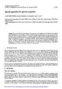
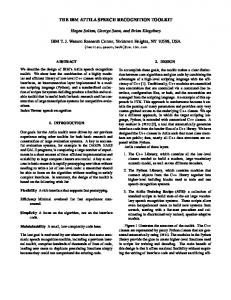
Table 3: Word error rates (percent) for grammar and acoustic constraints. ST-Same Talker, SG-Same Gender, DG-Different Gender. Conditions where our system performed as well or better than human listeners are bolded. same speaker are mixed together. This conditions best illustrates the importance of temporal constrains. By adding the acoustic dynamics, performance is improved considerably. By combining grammar and acoustic dynamics, performance improves again, surpassing human performance in the −3 dB condition. The second plot in Figure 1 shows WER for the Same Gender condition. In this condition, recordings from two different speakers of the same gender are mixed together. In this condition our system surpasses human performance in all conditions except 6 dB and −9 dB. The third plot in Figure 1 shows WER for the Different Gender condition. In this condition, our system surpasses human performance in the 0 dB and −3 dB conditions. Interestingly, temporal constraints do not improve performance relative to GMM without dynamics as dramatically as in the same talker case, which underscores the importance of the short-time signal characteristics in this condition. The performance of our best system, which uses both grammar and acoustic-level dynamics, is summarized in Table 3. This system surpassed human lister performance at SNRs of 0 dB through −6 dB on average across all speaker conditions. Averaging across all SNRs, the system surpassed human performance in the Same Gender condition. Future research will address some of the limitations of the task and model. We do not yet know if the proposed techniques generalize well to more realistic task conditions, such as unknown speakers, less constrained grammars, and more natural mixing conditions. The model also scales poorly with more than two speakers, and such scenarios would call for further approximations. Based on these initial results, however, we envision that super-human performance over all conditions is within reach for the speech separation challenge.

7. References

c) Different Gender 100

0

ST SG DG All

−6 dB

−9 dB

Grammar dyn.

Human

Figure 1: Word error rates for the a) Same Talker, b) Same Gender and c) Different Gender cases.

Figure 1 shows results for the 3 different conditions. Human listener performance [1] is shown along with the performance of the SDL recognizer without separation, GMM without dynamics, using acoustic level dynamics, and using both grammar and acoustic-level dynamics. The top plot in Figure 1 shows word error rates (WER) for the Same Talker condition. In this condition, two recordings from the

[1] Martin Cooke and Tee-Won Lee, “Interspeech speech separation challenge,” http : //www.dcs.shef.ac.uk/ ∼ martin/SpeechSeparationChallenge.htm, 2006. [2] T. Kristjansson, J. Hershey, and H. Attias, “Single microphone source separation using high resolution signal reconstruction,” ICASSP, 2004. [3] S. Roweis, “Factorial models and refiltering for speech separation and denoising,” Eurospeech, pp. 1009–1012, 2003. [4] P. Varga and R.K. Moore, “Hidden markov model decomposition of speech and noise,” ICASSP, pp. 845–848, 1990. [5] J.-L. Gauvain and C.-H. Lee, “Maximum a posteriori estimation for multivariate Gaussian mixture observations of Markov chains,” IEEE Transactions on Speech and Audio Processing, vol. 2, no. 2, pp. 291– 298, 1994. [6] Peder Olsen and Satya Dharanipragada, “An efficient integrated gender detection scheme and time mediated averaging of gender dependent acoustic models,,” in Proceedings of Eurospeech 2003, Geneva, Switzerland, September 1-4 2003, vol. 4, pp. 2509–2512.