the impact of priority generations in a multi-priority queueing system

Proceedings of the 2009 Winter Simulation Conference M. D. Rossetti, R. R. Hill, B. Johansson, A. Dunkin, and R. G. Ingalls, eds.

THE IMPACT OF PRIORITY GENERATIONS IN A MULTI-PRIORITY QUEUEING SYSTEM - A SIMULATION APPROACH

A. Krishnamoorthy

Viswanath C. Narayanan

Department of Mathematics Cochin University of Science and Technology Kochi 682022, India

Department of Mathematics Government Engineering College Sreekrishnapuram, 679 513, India

Srinivas R. Chakravarthy

ABSTRACT

Department of Industrial and Manufacturing Engineering Kettering University, Flint, MI 48504, USA.

In this paper, we consider a preemptive (multiple) priority queueing model in which arrivals occur according to a Markovian arrival process (MAP). An arriving customer belongs to priority type i, 1 ≤ i ≤ m + 1, with probability pi . The highest priority, labeled as 0, is generated by other priority customers while waiting in the system and not otherwise. Also, a customer of priority i can turn into a priority j, j 6= i, 1 ≤ i, j ≤ m + 1, customer, after a random amount of time that is assumed to be exponentially distributed with parameter depending on the priority type. The waiting spaces for all but priority type m + 1 are assumed to be finite. The (m + 1) − st priority customers have unlimited waiting space. At any given time, the system can have at most one highest priority customer. Thus, all priority customers except the (m + 1) − st are subject to loss. Customers are served on a first-come-first-served basis within their priority by a single server and the service times are assumed to follow a phase type distribution that may depend on the customer priority type. This queueing model, which is a level-dependent quasi-birth-and-death process, is amenable for investigation algorithmically through the well-known matrix-analytic methodology. However, here we propose to study through simulation using ARENA, a powerful simulation software as some key measures such as the waiting time distributions are highly complex to characterize analytically. The simulated results for a few scenarios are presented. 1

INTRODUCTION

While priority queues (both pre-emptive and non pre-emptive) have been extensively studied (see Takagi (Takagi 1989), Jaiswal (Jaiswal 1968) and references therein) in the literature, in this paper we analyze a multi-priority queueing system attended by a single server in which arriving priority customers can change their priorities while waiting for service. Such priority queueing models have been motivated by applications in areas such as health care and communication, and are referred to as self-generated priority queues. Self generation of priorities is a common phenomenon. For example, patients waiting in a clinic can become seriously ill and therefore given preference over other waiting patients. The change of priorities also takes place in multi-speciality hospitals. For example a patient waiting for an appointment with a physician specialized in a certain ailment, may require other specialized treatments. This patient may turn out to be critically ill at which time becomes a super-priority type requiring immediate attention in the current place (pre-empting the other priority customer in service) or elsewhere (due to another highest priority in service) by leaving the system. One can also find applications of the present model in communication, aircraft landing and so on. Krishnamoorthy, Deepak and Viswanath (Krishnamoorthy, Deepak, and Narayanan 2002) introduced self-generation of priority into queueing models. Wang (Wang 2004) discusses patient queue models with self-generation of priorities (though he does not introduce that terminology). He assumes all time variables to be exponentially distributed. Krishnamoorthy, Viswanath and Deepak (Krishnamoorthy, Narayanan, and Deepak 2005) provide an extensive analysis of a multiserver queue with Poisson arrival process. Customers while joining the system, are categorized as being ordinary; however while waiting they generate into priority according to a linear rate. The system is shown to be always stable. Several performance measures are computed. Some optimization problems are discussed. Gomez Corral, Krishnamoorthy and Viswanath (Gomez, Krishnamoorthy, and Narayanan 2005) analyzed a multi-server queueing system with a finite buffer and self-generation of priorities by waiting customers. Customers, at the time of joining the system, belong to one class and while waiting generate

978-1-4244-5771-7/09/$26.00 ©2009 IEEE

1622

Krishnamoorthy, Narayanan, and Chakravarthy into priority. They provide formulae for numerical computation of variety of performance measures, including the blocking probability, the departure process and the stationary distributions of the system state at pre-arrival epochs, post arrival epochs and epochs at which arriving customers are lost. In this paper, we consider a queueing system with m + 2 priorities, labeled as 0, 1, 2, . . .,m + 1, with 0 designated as super or highest priority and the rest of the m + 1 priorities are such that type i has a higher priority over type j customers, for i < j. We assume that the customers arrive according to a Markovian arrival process with parametric representation given by (D0 , D1 ) of order n. A brief description of MAP is given below. An arriving customer belongs to type i priority with probability pi , 1 ≤ i ≤ m + 1. The maximum capacity for priority type i is Ni with N0 = 1, Ni is finite for 1 ≤ i ≤ m and Nm+1 is infinite. An arriving priority i customer has one of the following options. (a) Enters into service immediately due to the server being idle or busy with a customer whose priority type is lower than that of the arrival; (b) Enters into priority i buffer if the buffer is not full (unless i = m + 1 in which case the customer will always enter into the buffer of infinite size); (c) Leaves the system since priority i buffer is full. Note that option (c) is not pertinent to type m + 1 customers as there is no limit for how many such customers can be admitted. It is easy to see that the priority i customers arrive according to a Markovian arrival process with the arrivals governed by the matrix D˜ i = pi D1 , 1 ≤ i ≤ m + 1. In our model, we assume that the highest priority customers do not arrive externally. Instead these customers are generated randomly by the other types of priority customers while waiting for service. In general, the priority generation scheme is as follows. After a random amount of time that is exponentially distributed with parameter γii , a priority type i, 1 ≤ i ≤ m + 1, customer waiting for service can γ turn into a highest priority with probability γγi0ii or into priority j, j 6= i, with probability γiiij . Note that γii = ∑m+1 j6=i, j=0 γi j , for 1 ≤ i ≤ m + 1, and that all priority i, 1 ≤ i ≤ m + 1, customers will independently change their priority type while waiting for service. We assume that while in service the customer cannot change the priority type. Furthermore, a highest priority customer finding another highest priority customer in service will leave the system without getting service and this is the reason why we take N0 = 1. Thus, the set {γi j , 1 ≤ i ≤ m + 1, 0 ≤ j ≤ m + 1}, along with the numbers of customers of priority type i, 1 ≤ i ≤ m + 1 will completely describe the self-priority generating scheme. The customers of priority type i have pre-emptive priority over customers of type j for i < j, 0 ≤ i, j ≤ m + 1. The pre-empted customer will be served (as a new customer) when the service begins for this customer following the priority rule. The service time of a customer of priority type i, 0 ≤ i ≤ m + 1, is assumed to be of phase type (PH-type) with representation (α(i), S(i)) and of order ri , where α(i) is the initial probability vector. S0 (i) is a column vector such that S(i)e + S0 (i) = 0, where e is a column vector of 1’s of appropriate order. Denoting by µi0 to be the mean of (α(i), S(i)), it can be verified that µi0 = −α(i)(S(i))−1 e. Recall that a PH-distribution is the distribution of the time until absorption in a continuous time Markov chain with an absorbing state (Neuts 1981). Observe that by taking γi j = 0 for 1 ≤ i ≤ m + 1; 0 ≤ j ≤ m + 1, we get the classical priority queue. On the other hand letting γi j 6= 0 for i ≤ j and γi j = 0 otherwise, the case of priority generation will be restricted to generating only one of higher priority. Similar interpretation (for generating one of lower priority) holds good when γi j 6= 0 for j ≥ i, i 6= 0. The MAP in continuous time is described as follows. Let the underlying Markov chain be irreducible and let Qˆ be the generator of this Markov chain. At the end of a sojourn time in state i, that is exponentially distributed with parameter λi , one of the following two events could occur: with probability ri j (1) the transition corresponds to an arrival and the underlying Markov chain is in state j with 1 ≤ i, j ≤ n; with probability ri j (0) the transition corresponds to no arrival and the state of the Markov chain is j, j 6= i. Note that the Markov chain can go from state i to state i only through an arrival. Define matrices D0 = (di0j ) and D1 = (di1j ) such that dii0 = −λi , 1 ≤ i ≤ m, di0j = λi ri j (0), for j 6= i and di1j = λi ri j (1), 1 ≤ i, j ≤ n. Note that for all i, 1 ≤ i ≤ n, ∑nj=1 [ri j (0) + ri j (1)] = 1. By assuming D0 to be a nonsingular matrix, the interarrival times will be finite with probability one and the arrival process does not terminate. Hence, we see that D0 is a stable matrix. The ˆ then the arrival rate λ is given generator Qˆ is then given by Qˆ = D0 + D1 . If π is the steady-state probability vector of Q, by λ = πD1 e, where e is a column vector of 1’s of dimension n. Thus, D0 governs the transitions corresponding to no arrival and D1 governs those corresponding to an arrival. It can be shown that MAP is equivalent to Neuts’ versatile Markovian point process. The point process described by the MAP is a special class of semi-Markov processes. For further details on MAP and their usefulness in stochastic modeling, we refer to ((Lucantoni 1991), (Neuts 1989), (Neuts 1992)) and for a review and recent work on MAP we refer the reader to (Chakravarthy 2001). The objective of this paper, therefore, is to generalize the classical priority queues. Of course we do this with restriction placed on the waiting spaces for all but the lowest priority one. This paper is presented as follows. In Section 2 we provide the description of the queueing model under study. In Section 3 we simulate this queueing model using ARENA, and discuss some illustrative numerical examples to qualitatively describe the model.

1623

Krishnamoorthy, Narayanan, and Chakravarthy 2

MODEL DESCRIPTION

The model described in the introduction can be studied using continuous time Markov chain as follows. First let Ji (t), 0 ≤ i ≤ m + 1, denote the number of type i priority customers in the system at time t. Let I1 (t) denote the state of the server with the convention that I1 (t) = 0 when the server is idle, and I1 (t) will be the phase of the existing service when the server is busy at time t; and let I2 (t) denotes the phase of the arrival process at time t. The process {H(t) : t ≥ 0} defined as {H(t) = (Jm+1 (t), Jm (t), . . . , J1 (t), J0 (t), I1 (t), I2 (t)) : t ≥ 0} is a continuous-time Markov chain with state space given by Ω = ∪∞ k=0 l(k), where l(0) = {(0, 0, . . . , 0, i2 ) |1 ≤ i2 ≤ n} ∪ {(0, jm , . . . , j0 , i1 , i2 )| m

0 ≤ jq ≤ Nq , 0 ≤ q ≤ m;

∑ ju 6= 0, 1 ≤ i1 ≤ rh , 1 ≤ i2 ≤ n, h = min0≤u≤m { ju > 0}},

u=0

l(k) = {(k, jm , jm−1 , . . . , j1 , j0 , i1 , i2 ) | 0 ≤ jq ≤ Nq , 0 ≤ q ≤ m; 1 ≤ i1 ≤ rh , 1 ≤ i2 ≤ n, h = min0≤u≤m+1 { ju > 0} , k ≥ 1. l(k), k ≥ 0 is referred to as the level k containing set of states. Note that in l(k) description it is obvious that jm+1 = k. It is clear that the above continuous time Markov chain {H(t)} is a level dependent quasi birth and death process (LDQBD). Arranging the states lexicographically the infinitesimal generator Q = (qrs ) of the process {H(t) : t ≥ 0} is given by   A10 A00  A20 A11 A0     A A A 22 12 0 Q= .   A A A 23 13 0   .. .. .. . . . The (block) matrices appearing in Q require extensive notations and since these are not absolutely necessary for our further discussion in this paper, the details are omitted here. Note that the system under discussion is always stable. It may be noted that setting γm+1, j = 0 for j = 0, 1, . . . , m, results in a level independent quasi birth and death process. In this case we get the infinitesimal generator of the process as a quasi-Toeplitz Markov chain and so the matrix geometric solution procedure can be adopted. 3

SIMULATION OF THE MODEL

The queueing model described in Section 2 is amenable to study through the classical algorithmic methods due to Neuts (Neuts 1981, Neuts 1989). However, we have chosen to simulate this queueing model using ARENA as the state space for the current model grows exponentially and the book-keeping becomes very intensive. Furthermore, the computation of the distributions of the waiting time in the system of various priority types (except the highest priority one) is very complicated to describe analytically. Thus, simulation will not only help to compare analytical results with those of the simulated ones, especially when one wants to generalize the model to include multiple-server case, but also get a feel for the waiting time distributions. The logic for developing the model is displayed in Figure 3 in the appendix. The ARENA modules for developing the model under study are displayed in Figures 4 and 5 in the appendix. The purpose of this section is to bring out the qualitative aspects of the queueing system under consideration through some interesting simulated (numerical) examples. For our numerical discussions, we consider five different arrival processes with parameter matrices D0 and D1 given by 1. Erlang of order 3 (ERL) 

−3 D0 =  0 0

3 −3 0

  0 0 3  , D1 =  0 −3 3

1624

0 0 0

 0 0  0

Krishnamoorthy, Narayanan, and Chakravarthy

2. Exponential (POI): D0 =

−1




, D1 =

1




3. Hyperexponential (HEX): 

−12.7 0 D0 =  0

  0 0 8.89  , D1 =  0.889 −1.27 0 0 −0.127 0.0889

2.54 0.254 0.0254

 1.27 0.127  0.0127

4. MAP with negative correlation (MNC): 

   −1.00222 1.00222 0 0 0 0  , D1 =  0.01002 0 0.9922  0 −1.00222 0 D0 =  0 0 −225.75 223.4925 0 2.2575 5. MAP with positive correlation (MPC): 

  −1.00222 1.00222 0 0  , D1 =  0.9922 0 −1.00222 0 D0 =  0 0 −225.75 2.2575

 0 0 0 0.01002  . 0 223.4925

All these five MAP processes are normalized so as to have an arrival rate of 1. However, these are qualitatively different in that they have different variance and correlation structure. The first three arrival processes, namely ERL, EXP, and HEX, correspond to renewal processes and so the correlation is 0. The arrival process labelled MNC has correlated arrivals with correlation between two successive inter-arrival times given by -0.4889 and and the arrivals corresponding to the processes labelled MPC has a positive correlation with values 0.4889. The ratio of the standard deviations of the inter-arrival times of these five arrival processes with respect to ERL are, respectively, 1, 1.732051, 5.913554, 2.44136, and 2.44136. For services we consider two cases: • •

ERL5: Here we assume that all five priorities have the same service distribution given by Erlang of order 5. We take µi0 = 0.9, 0 ≤ i ≤ 4. ERLV: Here we assume that the five priorities have different service distributions with the highest priority having Erlang of order 5; customers of priority type i have Erlang of order 5 − i, 1 ≤ i ≤ 4. Here we normalize the rates in each phase of the five Erlangs such that µi0 = 0.9, 0 ≤ i ≤ 4.

Note that Erlang is a special case of a phase type distribution. It should be pointed out that Erlang is a built-in distribution in ARENA. However, we have provided the module in ARENA as displayed in Figure 2 for using phase type services (of order 3) as this is not available in ARENA. In the following we will denote by γi the vector of dimension 5 that gives the rates of priority generation of a waiting priority i, 1 ≤ i ≤ 4 customer. That is, γi = (γi0 , . . . , γi4 ). In all our examples below we have fixed λ = 1, µi0 = 0.9, 0 ≤ i ≤ 4, pi = 0.25, 1 ≤ i ≤ 4, and γ1 = (1.5, 5, 1.5, 1, 1), γ2 = (2, 1.5, 6, 1.5, 2), γ3 = (2, 1.5, 1, 5.5, 1), γ4 = (3.5, 2, 2, 1.5, 9), N1 = 10, N2 = 20, and N3 = 30. We define the following measures (in steady state) for our discussion on the simulated results. (i)

•

µW T S , 0 ≤ i ≤ m + 1 the mean waiting time in the system of an admitted priority i customers (except for the priority m + 1 customers who will always be admitted due to unlimited buffer size. (i) Pbusy , 0 ≤ i ≤ m + 1 the probability that the server is busy with priority i customers at an arbitrary time.

•

Plost , 0 ≤ i ≤ m the probability that a priority i customer will be lost due to lack of buffer space at an arbitrary time.

•

sW T S , 0 ≤ i ≤ m + 1 the standard deviation of the waiting time in the system of an admitted priority i customer (except for the priority m + 1 customers who will always be admitted due to unlimited buffer size. (i) µNQ , 0 ≤ i ≤ m + 1 the mean number of priority i customers waiting in the queue at an arbitrary time.

•

•

(i)

(i)

1625

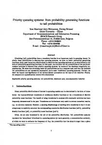
Krishnamoorthy, Narayanan, and Chakravarthy For the above combinations of five arrival processes and two service schemes, we ran our simulation model for 10000 units and five replications. The above set of performance measures along with the half-widths of the intervals are displayed in Tables 1 and 2 below. Furthermore, three selected measures: log of the mean waiting time in the system of customers of various priorities, the probability that the server is busy with different types of customers, and the probability of a priority i, 0 ≤ i ≤ 3, customer is lost, are displayed in Figure 1. A quick look at the entries in Tables 1, 2, and Figure 1, reveal the following observations. 1.

2.

3.

4.

5.

6.

7.

The mean waiting time for the highest priority customer entering into service (remember that a highest priority customer may leave without getting service due to server being busy with another highest priority customer) is nothing but the mean service time and is assumed to be the same, namely 0.90, for all scenarios. The numbers are very close to 0.9. This fact can also be used as an accuracy check for simulated results. The mean waiting time in the system for the lowest priority, namely, priority type 4, is largest among all customers and for all scenarios. This is as expected since these customers enter into the system without getting lost, and also are pre-empted by other priority customers. It is interesting to see that in the case of renewal arrivals (namely, when comparing ERL, POI, and HEX), the probability that the server is busy with priority i, 0 ≤ i ≤ 2, customers appears to increase with increasing variability in the arrival process. However, the probability that the server is busy with priority i, 3 ≤ i ≤ 4, customers appears to decrease with increasing variability in the arrival process. Looking at the probability that the server is busy with a specific priority type customer for the two correlated arrival processes, namely, MNC and MPC, we notice an interesting trend. For MPC process, this probability is larger as compared to MNC process in the case highest priority as well as for the lowest priority (priority 4) customers . However, for the other priority types, this probability is higher for MNC as compared to MPC. We notice that a priority 3 customer has the highest probability of getting lost when the arrival process has a larger variability (HEX) or has a higher positively correlated arrivals (MPC). It is not surprising to see this phenomenon since these customers have a limited waiting space and are probably pre-empted more often (next only to priority 4 customers). As is to be expected all the performance measures for renewal arrivals, namely, for ERL, POI, and HEX arrival processes, behave similar to what is to be expected. For example, the mean and standard deviation of the waiting times tend to increase with increasing variability. While MNC and MPC arrival processes have the same mean and standard deviation, yet some of the key measures such as the mean waiting times in the system of priority i, 1 ≤ i ≤ 4, customers are significantly different. This indicates the crucial role played by the correlated, especially the positive one, arrivals in stochastic modeling. We have seen such a crucial role played by the correlated arrivals in our other stochastic models analyzed using analytical and computational modeling tools.

Now we look at the fitted distributions of the waiting time distributions of various types of customers. Using the simulated data, ARENA has the option to identify the best fit (based on the least sum of squares due to error) among many distributions. In Tables 3 and 4 we list the fitted distributions for the various scenarios considered. Some sample histograms of simulated data along with the fitted distributions are displayed in Figure 2. An examination of these tables reveal the following. • •

•

As expected an admitted highest priority customer’s waiting time in the system is nothing but the service time distribution which is assumed to be Erlang of order 5. It is worth noting that the waiting time distribution of a priority 4 customer is fitted using beta distribution for all scenarios. As is known, the beta distribution has the ability to fit a variety of shapes in the data, and due to priority 4 customers having more chances of getting pre-empted by other types of customers and they all leave the system only after getting a service, the waiting times have more variability. Normally the waiting time distribution in a queueing model is skewed to the right (to accommodate for some customers having to wait unusually longer than the others) and this can be seen in ARENA identifying lognormal distribution to be the best fit for many combinations.

In conclusion, we have shown how simulation (using powerful software such as ARENA) can be used to bring out the qualitative aspect of a complicated stochastic model. Further research is currently being done to incorporate interesting optimization problems and the results of which will be presented elsewhere.

1626

1627

Utilization

(2) Pbusy (3) Pbusy (4) Pbusy (0) Plost (1) Plost (2) Plost (3) Plost (4) Plost (0) sW T S (1) sW T S (2) sW T S (3) sW T S (4) sW T S (0) µNQ (1) µNQ (2) µNQ (3) µNQ (4) µNQ

Pbusy

(1)

PERFORMANCE MEASURES (0) µW T S (1) µW T S (2) µW T S (3) µW T S (4) µW T S (0) Pbusy 0.00454 0.00318 0.00215 0.00005 0.00000 0.00000 0.00000 0.00000 0.00539 0.04021 0.12466 0.55645 61.895 0.00000 0.00370 0.01324 0.09616 27.29 0.00060

0.25160 0.10157 0.00002 0.00000 0.00000 0.00000 0.00000 0.40518 0.60279 1.49160 10.52700 1703.900 0.00000 0.05449 0.16401 1.81620 810.90 0.99930

0.00316

0.27233

0.28595

1044.10 0.99918

4.29360

0.33125

0.07567

0.00002 0.00000 0.00000 0.00022 0.00000 0.40008 0.67808 2.36370 18.41000 1943.400 0.00000

0.07512

0.24732

0.27188

0.29775

70.78 0.00100

1.35590

0.03108

0.00391

0.00005 0.00000 0.00000 0.00037 0.00000 0.00953 0.02943 0.21876 4.79220 126.670 0.00000

0.01148

0.00523

0.00791

0.00566

1605.20 0.99828

19.60900

4.17350

0.43384

0.00007 0.00015 0.01263 0.11258 0.00000 0.40220 2.06340 18.60100 80.58800 2343.400 0.00000

0.02831

0.18224

0.28493

0.33614

111.44 0.00236

1.76530

0.74292

0.06275

0.00009 0.00018 0.00461 0.02405 0.00000 0.00943 0.21219 10.53000 12.86400 402.370 0.00000

0.01466

0.01509

0.00993

0.01369

Table 1: Selected performance measures for various arrival processes ERL POI HEX 1 1 1 Average width Average width Average 2 2 2 width 0.90756 0.02792 0.89548 0.01722 0.90422 0.00946 1.08160 0.01754 1.14330 0.01452 2.14750 0.13259 1.73220 0.04678 2.37880 0.08655 15.19600 2.01650 8.77580 0.30126 18.20300 4.91690 100.29000 14.77000 2877.3 52.1 3536.1 460.5 4434.8 581.5 0.08855 0.00206 0.10793 0.00341 0.16838 0.00439

1256.90 0.99977

7.92000

0.45089

0.10087

0.00004 0.00000 0.00000 0.00191 0.00000 0.39840 0.77300 2.66550 26.69500 2511.500 0.00000

0.04442

0.24858

0.27736

0.31028

106.43 0.00024

2.37130

0.05529

0.00848

0.00006 0.00000 0.00000 0.00177 0.00000 0.01183 0.04281 0.22961 6.10350 424.850 0.00000

0.01725

0.00606

0.00678

0.01039

with identical services MNC 1 Average 2 width 0.89749 0.00987 1.21680 0.02993 2.80730 0.22619 31.60900 9.08760 3653.8 395.7 0.11936 0.00414

442.16 0.97646

7.85640

2.10270

0.27306

0.00002 0.05685 0.05121 0.06803 0.00000 0.39609 3.68170 14.65800 49.29200 706.060 0.00000

0.19758

0.19546

0.22723

0.23606

340.15 0.05842

1.54490

0.39690

0.05099

0.00004 0.01862 0.02293 0.02245 0.00000 0.01138 1.19800 0.58972 6.77910 446.110 0.00000

0.01022

0.00856

0.00476

0.00612

MPC 1 Average 2 width 0.89685 0.01347 2.04990 0.10389 9.86290 1.01300 38.52200 7.68620 1636.6 1173.7 0.14368 0.00980 Krishnamoorthy, Narayanan, and Chakravarthy

1628

Utilization

(2) Pbusy (3) Pbusy (4) Pbusy (0) Plost (1) Plost (2) Plost (3) Plost (4) Plost (0) sW T S (1) sW T S (2) sW T S (3) sW T S (4) sW T S (0) µNQ (1) µNQ (2) µNQ (3) µNQ (4) µNQ

Pbusy

(1)

PERFORMANCE MEASURES (0) µW T S (1) µW T S (2) µW T S (3) µW T S (4) µW T S (0) Pbusy 0.00237 0.00521 0.01073 0.00020 0.00000 0.00000 0.00005 0.00000 0.01141 0.10778 0.13052 3.79110 282.89000 0.00000 0.00395 0.01983 0.60056 109.18000 0.00207

0.24886

0.10148

0.00020 0.00000 0.00000 0.00002 0.00000 0.39870 0.66169 1.75820 12.37900 1693.30000 0.00000

0.05255

0.19624

2.15810

824.81000 0.99916

0.00415

0.27076

0.28498

1160.30000 0.99960

6.85050

0.38750

0.08497

0.00014 0.00000 0.00000 0.00215 0.00000 0.39606 0.77892 2.67620 26.75200 2180.40000 0.00000

0.05890

0.24935

0.27672

0.30032

63.96900 0.00108

1.78490

0.04103

0.00544

0.00017 0.00000 0.00000 0.00235 0.00000 0.01114 0.04781 0.30742 6.29030 182.61000 0.00000

0.01270

0.00497

0.00642

0.00635

1539.20000 0.99696

18.66400

3.92510

0.42781

0.00022 0.00041 0.01027 0.10328 0.00000 0.40492 2.46970 13.49300 78.77300 2496.50000 0.00000

0.03327

0.18578

0.28172

0.33009

98.22300 0.00355

1.13870

0.56637

0.04049

0.00006 0.00038 0.00201 0.01841 0.00000 0.01747 0.94459 0.83433 14.04900 342.72000 0.00000

0.00703

0.01407

0.00814

0.01063

1246.60000 0.99965

6.83620

0.45598

0.09868

0.00022 0.00000 0.00000 0.00170 0.00000 0.39879 0.78382 3.29880 25.01700 2381.50000 0.00000

0.05041

0.24990

0.27497

0.30500

78.94900 0.00043

0.89532

0.03062

0.00704

0.00013 0.00000 0.00000 0.00163 0.00000 0.00654 0.03022 1.22750 3.62690 169.06000 0.00000

0.00563

0.00583

0.00402

0.00860

632.31000 0.99380

9.83460

2.66370

0.34065

0.00005 0.06572 0.06205 0.07942 0.00000 0.39831 3.88800 15.84900 50.46400 1093.50000 0.00000

0.17019

0.20321

0.23265

0.24706

230.81000 0.00806

1.56240

0.42103

0.05452

0.00005 0.01012 0.01065 0.01135 0.00000 0.01327 2.62360 1.04690 3.23130 454.74000 0.00000

0.02161

0.00324

0.00583

0.01132

Table 2: Selected performance measures for various arrival processes with different service distributions ERL POI HEX MNC MPC 1 1 1 1 1 width width width width Average Average Average Average Average 2 2 2 2 2 width 0.90426 0.01429 0.89510 0.00786 0.90251 0.01187 0.88986 0.02266 0.90120 0.01712 1.07530 0.01838 1.17430 0.02514 2.16110 0.08350 1.20870 0.02397 2.22400 0.19361 1.84300 0.07403 2.55730 0.13963 14.35600 1.52340 2.84320 0.10748 11.72200 1.51640 10.09300 2.15960 27.49300 6.41370 94.50000 11.50100 27.45300 3.48120 45.58200 6.89320 2903.70000 468.33000 3760.80000 367.97000 3946.40000 831.87000 4152.80000 806.50000 2099.40000 650.68000 0.09392 0.00472 0.11471 0.00500 0.16913 0.00307 0.11973 0.00434 0.14689 0.00383 Krishnamoorthy, Narayanan, and Chakravarthy

Krishnamoorthy, Narayanan, and Chakravarthy

Figure 1: Comparison of selected measures for various scenarios

ARRIVAL ERL POI HEX MNC MPC

Table 3: Identification of the fitted distributions for the waiting time in the system for identical services Highest Priority Priority 1 Priority 2 Priority 3 Priority 4 ERLANG(0.181, 5) LOGN(1.08, 0.607) LOGN(1.71, 1.41) 70 BETA(0.481, 3.36) 6060 BETA(0.933, 1.06) ERLANG(0.179, 5) LOGN(1.14, 0.676) LOGN(2.34, 2.34) 114 BETA(0.607, 3.19) 7270 BETA(1.15, 1.21) ERLANG(0.181, 5) LOGN(2.12, 2.11) EXP(15.2) 492 BETA(0.724, 3.83) 9310 BETA(1.61, 2.12) ERLANG(0.18, 5) LOGN(1.22, 0.766) LOGN(2.81, 2.93) 178 BETA(0.865, 4.03) 8680 BETA(0.805, 1.14) ERLANG(0.179, 5) W EIBULL(2.07, 0.935) LOGN(10.2, 35.1) LOGN(73.4, 697) 3990 BETA(0.802, 1.12)

ARRIVAL ERL POI HEX MNC MPC

Table 4: Identification of the fitted distributions for the waiting time in the system for varying services Highest Priority Priority 1 Priority 2 Priority 3 Priority 4 ERLANG(0.181, 5) GAMMA(0.324, 3.32) LOGN(1.85, 1.87) 98 BETA(0.458, 3.98) 6380 BETA(1.07, 1.3) ERLANG(0.179, 5) LOGN(1.18, 0.79) LOGN(2.58, 3.09) 146 BETA(0.622, 2.68) 8300 BETA(1.17, 1.42) ERLANG(0.181, 5) EXPO(2.16) 291 BETA(1.02, 19.6) 926 BETA(1.164, 10.3) 8670 BETA(0.83, 0.978) ERLANG(0.178, 5) LOGN(1.21, 0.818) GAMMA(0.823, 4.22) 168 BETA(0.823, 4.22) 8510 BETA(0.991, 1.09) ERLANG(0.18, 5) GAMMA(2.17, 1.03) LOGN(11.9, 43.6) LOGN(98.6, 824) 5490 BETA(1.6, 2.76)

1629

Krishnamoorthy, Narayanan, and Chakravarthy

Figure 2: Histograms and fitted distributions for waiting time in the system for selected scenarios

REFERENCES Chakravarthy, S. R. 2001. The batch Markovian arrival process: A review and future work. In Advances in Probability Theory and Stochastic Processes., ed. A. K. et al., 21–39. New Jersey: Notable Publications Inc.,. Gomez, C. A., A. Krishnamoorthy, and V. C. Narayanan. 2005. The impact of self-generation of priorities on multi-server queues with finite capacity. Stochastic Models 21 (2–3): 427–447. Jaiswal, N. 1968. Priority queues. New York: Academic Press. Krishnamoorthy, A., T. Deepak, and V. C. Narayanan. 2002. Queues with self-generation of priorities. Technical report, Cochin University of Science and Technology. Krishnamoorthy, A., V. C. Narayanan, and T. G. Deepak. 2005. On a queueing system with self generation of priorities. Journal of Neural Parallel and Scientific Computations. Lucantoni, D. 1991. New results on the single server queue with a batch markovian arrival process. Stochastic Models 7:1–46. Neuts, M. 1989. Structured stochastic matrices of m/g/1 type and their applications. NY: Marcel Dekker. Neuts, M. 1992. Models based on the markovian arrival process. IEICE Transactions on Communications E75B:1255–1265. Neuts, M. F. 1981. Matrix-geometric solutions in stochastic models: An algorithmic approach. Baltimore, MD: The Johns Hopkins University Press (Dover since 1994). Takagi, H. 1989. Queueing analysis - volume 1: Vacations and priority systems. Amsterdam: North-Holland. Wang, Q. 2004. Modeling and analysis of high risk patient queues. European J. Oper. Res. 155:502–515.

AUTHOR BIOGRAPHIES A. KRISHNAMOORTHY is Professor of Applied Mathematics at the Cochin University of Science & Technology, India, since January 1987. He received the Doctoral degree in 1978 and has over 100 research publications and has edited a few conference proceedings. He is Editor of OPSEARCH and is on the Editorial board of a number of journals. His areas of interest include Operations Research, Stochastic Modelling with special reference to Queues, Inventory and Reliability. His email address for these proceedings is . VISWANATH C. NARAYANAN is Lecturer in mathematics at Government Engineering College, Trissur, India. He has over 20 research publications. His areas of interest include Stochastic modeling in Queues, Inventory, Reliability and Bio-informatics. His email address for these proceedings is . SRINIVAS R. CHAKRAVARTHY is a Professor of Operations Research and Statistics in the Department of Industrial and Manufacturing Engineering at Kettering University, Flint, Michigan, USA. His research interest are in the areas of algorithmic probability, queuing, reliability and inventory. He has published more than 70 papers in leading journals and presented papers at national and international conferences. He co-organized the First and Second International Conferences on Matrix-analytic Methods in Stochastic Models in 1995 and 1998. He received Kettering University Alumni’s Outstanding Teacher Awards (1990 and 2001) and Kettering University’s Outstanding Researcher (1996) and Distinguished Researcher (2003) Awards. He is on the scientific advisory committee of several international conferences, and also on the editorial board of a few journals. His email address for these proceedings is .

1630

Krishnamoorthy, Narayanan, and Chakravarthy APPENDIX

LOGIC FOR DEVELOPING THE SIMULATION MODEL MAP arrivals

Leave w/o service

Determine priority

Seize server

Leave with service

Pre-empted Enter buffer Modulation of priorities of waiting customers. A customer becoming a super-priority (0) customer enters into service by possibly preChange in priority empting the one in service. The customer in service, if any, will either enter into buffer or leave the system due to lack of space.

Figure 3: Logic for the development of ARENA model

1631

Leave w/o service

Krishnamoorthy, Narayanan, and Chakravarthy

The Impact of Priority Generations in a Multi-priority Server Queueing system - A Simulation Approach (Krishnamoorthy, Viswanath, and Chakravarthy) MAP AR R IVALS

Ma in E ntra nc e P H - S ER VIC ES

Re c ord Ke e ping

Priority Generation

0

Tr ue

Qu e u e

Se rv e r b u s y fo r ty p e 1 ?

MAIN ENTRANCE

Pre e m p t

T Y P E 1 . Qu e u e

0

S E RV E R

Fals e

0

S E P A RA T E F OR DE CI DE O r igin al

0

0

Tr ue

Se rv e r b u s y fo r ty p e 2 ?

Qu e u e

A s s i g n P ri o ri t y

Ch o o s e b u ffe r

0

0

Fals e

Type==1 Type==2 Type==3

Els e

Ca n b u ff e r a c c o m m o d a te ?

As s i g n ty p e i n s e rv i c e

Tr ue

0

Tr ue

Se v e r b u s y f o r ty p e 3 ?

0

Duplic at e

Pre e m p t

T Y P E 2 . Qu e u e S E RV E R

Qu e u e

Fals e

0

Pre e m p t

T Y P E 3 . Qu e u e S E RV E R Fals e

T ra c k L o s t A s s i g n Nu m b e rs queue and s y s te m

T YPE 4 L OS T DUE T O B UF F E R F UL L

0 0

Pre e m p t

Tr ue

Se rv e r b u s y fo r ty p e 0 ? Di s p o s e

W HERE T O SEND SIGNAL ?

S E RV E R

0

0

Fals e Els e

Type == 1 && NQ ( TYPE 1. Q ueue) >= 1 Type == 2 && NQ ( TYPE 2. Q ueue) >= 1 Type == 3 && NQ ( TYPE 3. Q ueue) >= 1 Type == 4 && NQ ( TYPE 4. Q ueue) >= 1

PHASE TYPE SERVICES FR O M 1 TO W H E R E ? M AP Proc es s 1 Else

MAP ARRIVALS

0

ARRIVAL AND START IN 1

O rg in i al

Process 1

0

0

100* S MA T(1,2)/A BS (S MAT(1,1)) 100* S MA T(1,3)/A BS (S MAT(1,1)) E lse

M AP Pro c e s s 2

30 30

0

FROM STATE 1

Duplci at e

0

D E C ID E W H E R E TO G O?

M AP ARRIVAL S

100* D1M ( 1, 1) / ABS( D0M ( 1, 1) ) 100* D1M ( 1, 2) / ABS( D0M ( 1, 1) ) 100* D1M ( 1, 3) / ABS( D0M ( 1, 1) ) 100* D0M ( 1, 2) / ABS( D0M ( 1, 1) )

0

ARRIVAL AND START IN 2

FR O M 2 TO W H E R E ?

Else

Else

M AP Pro c e s s 3

100* D1M ( 2, 1) / ABS( D0M ( 2, 2) ) 100* D1M ( 2, 2) / ABS( D0M ( 2, 2) ) 100* D1M ( 2, 3) / ABS( D0M ( 2, 2) ) 100* D0M ( 2, 1) / ABS( D0M ( 2, 2) )

0

0 O rg in i al

INITIAL PROB VECTOR B T(1)*100 B T(2)*100

Duplci at e

Process 2

E lse

FROM STATE 2 100* SMAT(2,1)/AB S(S MA T(2,2)) 100* SMAT(2,3)/AB S(S MA T(2,2))

0 Else

0 ARRIVAL AND START IN 3

0

FR O M 3 TO W H E R E ?

Else

0 Org in i al

Duplci at e

100* D1M ( 3, 1) / ABS( D0M ( 3, 3) ) 100* D1M ( 3, 2) / ABS( D0M ( 3, 3) ) 100* D1M ( 3, 3) / ABS( D0M ( 3, 3) ) 100* D0M ( 3, 1) / ABS( D0M ( 3, 3) )

Process 3

0

FROM STATE 3 100* SMA T(3,1)/AB S (S MA T(3,3)) 100* SMA T(3,2)/AB S (S MA T(3,3)) E lse

Figure 4: ARENA MODULES - Main, MAP arrivals and Phase type services

1632

Krishnamoorthy, Narayanan, and Chakravarthy

SELF-PRIORITY GENERATIONS

SI GNAL F OR HOL D 1 DI SPOSE SI GNALS

SI GNAL F OR HOL D 2

0

SI GNAL F OR HOL D 3

0

Assign Type From GP 2

J OI N BUF F ER 2 OR Tr ue L EAVE?

SI GNAL F OR HOL D 4

0

Fals e

DI SPOSE2

HOL D F OR SI GNAL 1

GENERATE PRI OR 1

0

SEPARTE FOR HOLD 1

0

0

0 O rg in i al

ST AT E 1

ST AT E 1 T O 2 OR 3 OR HP

100* Q SR( 1, 2 ) / ABS( Q SR( 1, 1) ) 100* Q SR( 1, 3 ) / ABS( Q SR( 1, 1) ) 100* Q SR( 1, 4 ) / ABS( Q SR( 1, 1) )

Duplci at e Els e

GENERATE PRI OR 2

0

HOL D F OR SI GNAL 2

0

SEPARTE FOR HOLD 2

0

ST AT E 2

O rg in i al

GENERATE PRI OR 3

J OI N BUF F ER 1 OR Tr ue L EAVE?

ST AT E 2 T O 1 OR 3 OR HP

0

Assign Type From GP 1

Assing HP Type

Fals e

Dispose HP wti hout service

100* Q SR( 2, 1 ) / ABS( Q SR( 2, 2) ) 100* Q SR( 2, 3 ) / ABS( Q SR( 2, 2) ) Fals e 100* Q SR( 2, 4 ) / ABS( Q SR( 2, 2) )

Duplci at e

0

0

TRACK HP LOST DI SPOSE1

0

SEPARTE FOR HOLD 3

O rg in i al

0 0

0

An y o t h e r HP i n t h e Tr ue s y s te m ?

0

Els e

HOL D F OR SI GNAL 3

TRACK LP 2 LOST

ST AT E 3

Duplci at e

0

TRACK LP 1 LOST

ST AT E 3 T O 1 OR 2 OR HP

100* Q SR( 3, 1 ) / ABS( Q SR( 3, 3) ) 100* Q SR( 3, 2 ) / ABS( Q SR( 3, 3) ) 100* Q SR( 3, 4 ) / ABS( Q SR( 3, 3) )

Els e

0

GENERATE PRI OR 4

0

HOL D F OR SI GNAL 4

SEPARTE FOR HOLD 4

0

J OI N BUF F ER 3 OR Tr ue L EAVE?

0 O rg i n i al

ST AT E 4

0

Duplci at e

Assign Type From GP 3

Fals e

ST AT E 4 T O 1 OR 2 OR 3 OR HP 100* Q SR( 4, 1) / ABS( Q SR( 4, 4) ) TRACK LP 3 100* Q SR( 4, 2) / ABS( Q SR( 4, 4) ) 100* Q SR( 4, 3) / ABS( Q SR( LOS 4, 4)T )

Els e

DI SPOSE3

0

0

J OIN BUF F ER 4 OR L EAVE?

0

Tr ue

Assign Type From GP 4

Fals e

DI SPOSE4

TRACK LP 4 LOST

0

RECORD KEEPING Dispose 1

0 0 HP or LP?

T ru e

S et NHP to 0

A S S IGN TY P E FOR LS

Dispose 2

0

Fa ls e

0

Write Priority 1 RELEASE SERVER

WRITE TO PRIORITY 0?

Els e

RE CORD WTS

T YPE T YPE T YPE T YPE

L E A V I NG L E A V I NG L E A V I NG L E A V I NG

S E R V I CE = = 1 S E R V I CE = = 2 S E R V I CE = = 3 S E R V I CE = = 4

Write Priority 2

Dispose 3

DECIDE WHICH TYPE IS LEAVING

El s e

T YPE T YPE T YPE T YPE

L E A V I NG L E A V I NG L E A V I NG L E A V I NG

S E RV I CE = = 1 S E RV I CE = = 2 S E RV I CE = = 3 S E RV I CE = = 4

0

DIS P OS E 4

0

Write Priority 3

DIS P OS E HP

0 Write Priority 4

Write Priority 0

Figure 5: ARENA MODULES - Self-priority generation and Record keeping

1633