The inclusion of exogenous variables in functional autoregressive ...

ISUP - LSTA

2001-4

Juin 2001

The inclusion of exogenous variables in functional autoregressive ozone forecasting

Julien DAMON et Serge GUILLAS

Rapport Technique n◦ 4 (2001)

Institut de Statistique de l’Universit´e de Paris Laboratoire de Statistique Th´eorique et Appliqu´ee Universit´e Paris VI Tour 45-55, Boˆıte 158 4, place Jussieu 75252 Paris Cedex 05

Rapport Technique n◦ 4 (2001)

The inclusion of exogenous variables in functional autoregressive ozone forecasting

Julien DAMON et Serge GUILLAS Universit´e Paris VI, ISUP-LSTA Tour 45-55, Boˆıte 158 4, place Jussieu, 75252 Paris Cedex 05

Juin 2001

Ces documents de travail n’engagent que leurs auteurs. Working papers only reflect the views of the authors.

The inclusion of exogenous variables in functional autoregressive ozone forecasting J. Damon

S. Guillas

Universit´e Paris 6

Universit´e Paris 6 Ecole des Mines de Douai

Juin 2001

Abstract In this paper, we propose a new technique for ozone forecasting. The approach is functional, that is we consider stochastic processes with values in function spaces. We make use of the essential characteristic of this type of phenomena by taking into account theoretically and practically the continuous time evolution of pollution. One main methodological enhancement of this paper is the incorporation of exogenous variables (wind speed and temperature) in those models. The application is carried out on a six-year data set of hourly ozone concentrations and meteorological measurements from B´ethune (France). The study examines the summer periods because of the higher values observed. We explain the non parametric estimation procedure for autoregressive Hilbertian models with or without exogenous variables (considering two alternative versions in this case) as well as for the functional kernel model. The comparison of all the latter models is based on up-to-24 hour-ahead predictions of hourly ozone concentrations. We analyzed daily forecast curves upon several criteria of two kinds: functional ones, and aggregated ones where attention is put on the daily maximum. It appears that autoregressive Hilbertian models with exogenous variables showed the best predictive power.

1

Introduction

The prediction of atmospheric pollutants is a problem studied by a large community of researchers working in various scientific areas. Due to the inner complexity of the spatiotemporal phenomena and the parsimony of data, one may have a look at statistical techniques. Since basic models did not satisfy experts enough, statisticians created numerous models which can roughly be classified into three main approaches. Times series and regression models have been naturally and widely used, involving ARMA models with time-varying coefficients (Barrat et al. (1990)), threshold autoregressive models (M´elard and Roy (1988)), the two latter models with exogenous variables (Bauer et al. (2001)), GARCH models (Graf-Jacottet and Jaunin (1998)), linear regression models (Comrie and Diem (1999)), nonparametric regression models with eventually

1

a linear combination of exogenous variables (Gonzalez-Manteiga et al. (1993) and PradaSanchez et al. (2000)), nonparametric discriminant analysis and Multivariate Adaptive Regression Splines - MARS - (Silvia et al. (2001)), Generalized Additive Models -GAM(Davis and Speeckman (1999)), and chaotic time series (Kocak et al. (2000)). Another way of making prediction is to use neural networks. Boznar et al. (1993), Yi and Prybutok (1996), Gardner and Dorling (1999) and P´erez et al. (2000) considered the multilayer perceptron while Ruiz-Suarez et al. (1995) chose bidirectional associative memory and holographic associative memory models. Classification and regression trees models (Breiman et al. (1984)) showed good capacities in this field. Ghattas (1999) and Gardner and Dorling (2000) illustrated this approach. The idea of considering functional models comes from the observation of those phenomena. From a physical point of view, it is clear that the processes involved in the production of ozone are of continuous time type, therefore continuous time stochastic processes should be accurate to model the evolution of pollutants. The enhancement in the modelling procedure is the incorporation of exogenous variables in the AutoRegressive Hilbertian Model of order one - denoted by the acronym ARH(1) or simply ARH - giving as a result AutoRegressive Hilbertian Model of order one with exogenous variables denoted by the acronym ARHX(1) or simply ARHX. Such Hilbertian processes have been studied because they can handle theoretically and practically (for example by use of smoothing splines, see Besse and Cardot (1996)) a large number of continuous time processes. Our approach is a functional one, as curves are our object of study, see Ramsay and Silverman (1997) for a review of ”functional data analysis”, and Rice and Wu (2001) for a work in this field relatively close to ours but with a fixed basis of spline functions. In the next section, we will present the data and how we can measure correctness of forecasts. Then, we will introduce the various models and explain how the non parametric estimation procedures are working, in particular for cross validation. Finally, a comparison will permit to evaluate the qualities of the diverse approaches.

1.1

Pollution and weather data, associated criteria of accuracy for predictions

The data came from the so-called AREMARTOIS air quality authority for the Artois area in the north of France. Six years of data were used: the period range is from January 1st 1995 to December 31st 2000. The monitoring station collected information about ozone every 15 minutes, but the available data were the hourly averages. One weather monitoring station collected hourly measurements of temperature, wind speed and wind direction. Notice that missing values were essentially missing during entire months for technical reasons, only a few were missing during one hour or two for maintenance purposes. Therefore, our choice was not to replace the missing values with interpolated ones. We fitted the various models to data ranging from January 1st 1995 to December 31st 1999. We analyzed the predictions on the remaining year. Due to the missing 2

values which affect differently the various variables, the set of prediction days are slightly different, depending on the model used, but the comparisons are made on the days where each method provided results. The horizon of prediction is of 24 hours, but not in the usual sense. Every 11 p.m., we forecast the 24 values of the following day. This choice was made for simplicity purposes, but the model is relatively flexible regarding the hour when the prediction starts and the number of predicted values, as functional models can. The criteria used in the sequel are of functional type: we want to see if the entire predicted curve for one day is close to the real one. Considering our pollutant (ozone), let ˆ i,j the prediction of Xi,j . Xi,j be its concentration in µg/m3 of day j at hour i and X In order to compare the curves, we compute for integers p = 1, 2 respectively the following empirical Lp -errors on a sample of n days based on the discretization scheme

ˆ

X − X

L1



ˆ

X − X

L2

n 23 1 X 1 X ˆ = Xi,j − Xi,j , n 24 j=1 i=0 v u n 23  2 X 1 Xu t1 ˆ i,j − Xi,j . = X n 24 j=1

i=0

The L2 -error is much more sensitive to large errors during one day as might be possible during peak days of ozone. For p = ∞, we recall that the L∞ -error is calculated as

ˆ

X − X

n

L∞

=

1X ˆ sup X − X i,j i,j . n i=0,...,23 j=1

It is clearly possible to compute with this type of data and predictions the daily maximum or the 8h average level as required by the National Ambient Air Quality Standards in the USA. In France, a so-called ATMO index is calculated. It is the maximum of the partial ATMO indexes associated to O3 , NO2 , SO2 and particulate material, computed as a number between 1 and 10 representing intervals of maximum daily concentrations. The classical criteria we will use for these daily maxima are presented below. Data are real numbers and not of functional type as above, so if we denote (Xi )i=1,...,n the   ˆi observations and X the forecasts, we can compute i=1,...,n

• The Mean Squared Error (MSE) n

1X ˆ M SE = (Xi − Xi )2 n i=1

and the Root Mean Squared Error (RMSE) v u n u1 X ˆ i − Xi )2 RM SE = t (X n i=1

3

• The Mean Absolute Error (MAE) n 1 X ˆ M AE = Xi − Xi n i=1

• The Mean Relative Error (MRE) n

1X ˆ M RE = (Xi − Xi )/Xi n i=1

• The Mean Relative Absolute Error (MRAE) M RAE =

n 1 X ˆ Xi − Xi /Xi n i=1

Large errors of prediction clearly exert a bigger influence on the two squared errors M SE and RM SE than on the M AE. If the forecasts from one model are almost always correct but rarely very bad, this could be better for M AE but not for M SE and RM SE than another model with daily prediction errors of homogeneous size which makes worse predictions in general. Moreover, the relative errors must be regarded carefully when data are relatively close to 0. Since the ”persistence method” - that is the na¨ıve prediction which makes today’s curve the predicted one for tomorrow - appeared clearly not accurate on curves, we only focused on the following methods.

2

The models

Let H be a real and separable Hilbert space, e.g. H is L2 [0, 24] in our application. Denoting by (xt )t∈R the continuous time ozone process, we will consider the associated H-valued process (Xn )n∈Z defined by Xn (t) = x24n+t , t ∈ [0, 24] . In this way, we place the problem in a simpler discrete time context. (Xn ) will be the variable of interest in the following models, and we want to predict Xn+1 .

2.1

Autoregressive Hilbertian process

Let ρ be a bounded linear operator on H. Let (εn )n∈Z be a strong Hilbertian white noise (SWN), that is a sequence of i.i.d. H-valued random variables satisfying ∀n ∈ Z, Eεn = 0, 0 < E kεn k2H = σ 2 < ∞. (Xn ) is an ARH process defined as the unique stationary solution of Xn = ρ(Xn−1 ) + εn . 4

(1)

In order to the stationarity of (Xn ) and, we assume the standard hypothesis Pensure ∞ n on ρ, that is n=0 kρ k < ∞. We recall that under such conditions, limit theorems and consistent estimation are obtained (see Bosq (2000)). To produce one step ahead forecasts, we need to estimate ρ. The technique -as exposed in Bosq (2000)- proceeds as follows. Since the empirical estimator Cn of the covariance operator is not invertible in general, ρ’s empirical estimator ρn is computed in a subspace spanned by the kn eigenvectors of Cn associated to its kn greatest eigenvalues.

2.2

Autoregressive Hilbertian Model with exogenous variables

Keeping the same notations, let us introduce a1 , ..., aq bounded linear operators on H. We consider the following autoregressive Hilbertian with exogenous variables of order one model, denoted by ARHX(1): Xn = ρ(Xn−1 ) + a1 (Zn,1 ) + ... + aq (Zn,q ) + εn , n ∈ Z

(2)

where Zn,1 , ..., Zn,q are q zero-mean autoregressive of order one - ARH(1) - exogenous variables associated respectively to operators u1 , ..., uq and strong white noises (ηn,1 ) , ..., (ηn,q ), i.e. Zn,i = ui (Zn−1,i ) + ηn,i . (3) We assume that the noises (εn ), (ηn,1 ), ..., (ηn,q ) are independent and similar hypotheses on the various operators as in the previous section to ensure existence, limit theorems and consistent estimation. We choose to study ARHX(1) models in order to asses the influence of exogenous variables, considering this way an extension of the Granger causality in function spaces, see e.g. Guillas (2000) for theoretical results and Pitard and Viel (1999) for an illustration in an epidemiologic field with selection of exogenous variables using Granger-causality tests. One may write ARHX(1) models with exogenous processes taking their values in various spaces , i.e. Hi -valued Zn,i . In this paper, we prefer to use H-valued Zn,i for simplicity, knowing that proofs are similar to the general case. We will use the autoregressive representation of the equation (2) in a product space in order to compute our estimates. 2.2.1

Autoregressive representation

The following construction enables us to manage ARHX processes as ARH processes, and thereby adapt the technique of estimation. As Mourid (1995) did for ARH(p) processes, we consider the Cartesian product H q+1 of q + 1 copies of H equipped with the scalar product q+1 X h(x1 , ..., xq+1 ) , (y1 , ..., yq+1 )iq+1 := hxj , yj i . j=1

H q+1 is then a separable Hilbert space. 5

Let us denote 

  Tn =  

Xn Zn+1,1 .. . Zn+1,q





   0   , εn =   

εn ηn,1 .. . ηn,p



ρ a1  0 u1     0  , and ρ =   0 0   .. ..  . . 0 0 

··· 0

··· ···

u2

0 .. .

0

0

aq 0 .. .



   .   0  uq

Let (Xn ) be an ARHX(1) defined by (2), then it can easily be proved that (Tn ) is an H q+1 -valued ARH(1) process (it is the unique stationary solution to the following equation): Tn = ρ0 (Tn−1 ) + ε0n (4) In practice, we will compute estimators of eigenvalues and eigenvectors of the covariance operator CnT concerning the H q+1 -valued ARH(1) process (Tn ). 2.2.2

Two variants of the ARHX model

As stated in the introduction, we want to improve the ARH model by incorporating exogenous variables. Thus, we consider (with q = 2) the ARHX model (2) where Xn , Zn,1 and Zn,2 represent respectively centered ozone concentration, temperature and wind speed. Two approaches are at least possible, in order to estimate this ARHX. The first one is simply to apply the theoretical techniques exposed previously, that is represent the process and the exogenous variables in a vector of H q+1 as shown in equation (4). This model will be denoted by the acronym ARHX(a). The second is a empirical improvement of the previous one. It aims to get rid of the important reproductive behavior of the ARH model. In this way, we want to take into account better the exogenous variables’ influence on our variable of interest. To estimate an ARHX, our approach is to consider an finite subspace in which we project the observations, in order to inverse the covariance operator CnT . Indeed, there is no obligation to use the kn eigenvectors of CnT associated to the kn greatest eigenvalues so we propose here an alternative choice for this subspace. Rather than considering Tn as a simple ARH model, we adapt the estimation to its known inner structure. To do so, we decompose H q+1 in q + 1 spaces H. In each space H, linked to a variable (X, or a Zi , i = 1, ...q), we choose (as in the ARH model) the subspace generated by the eigenvectors of the appropriate covariance operator (of X, or a Zi , i = 1, ...q) associated to the greatest eigenvalues. The resulting basis for our subspace in H q+1 is therefore spanned

6

by vectors of the following form              

v11 0 .. . .. . .. . .. . 0





             , ...,             

v 1(1) kn

0 .. . .. . .. . .. . 0





            , ...,            



0 0  . ..   .. .     0 0     vi v1i  , ...,  kn(i)   0   0   ..   .. .   . 0 0 





0 .. . .. . .. . .. . 0

             , ...,            

v1q+1

(1)





             , ...,             

0 .. . .. . .. . .. . 0 v q+1 (q+1) kn



      .      

(2)

In this way, we get kn vectors with non zero coefficients in line 1, kn vectors with non (q+1) zero coefficients in line 2, ..., kn vectors with non zero coefficients in line q + 1. Hence, we control the evolution space of our different variables : we can then isolate the effect of Zi in the estimated matrix ρ0n of ρ0 and adapt the subspace independently for each (i) variable using the kn . If we had not done so, the subspace obtained (by the eigenvectors of CnT ) would have been drastically designed by the autoregressive part of the interest variable. The practical disadvantage of this approach is that we now have to choose q + 1 (1) (q+1) parameters kn , ..., kn , and cross validation procedure is much more complicated. This model will be denoted by the acronym ARHX(b).

2.3

Functional kernel model

Although the ARH model is non parametric, it assumes the linearity of ρ. To get rid of such an assumption, we applied a functional kernel modelling as follows. An alternative approach is to consider a local ARH predictor where local estimates of covariance and cross covariance operators are computed using kernel techniques as in Besse et al. (2000). One nonparametric way to deal with the conditional expectation ρ(x) = E [Xi |Xi−1 = x ], where (Xi ) is a H-valued process, is to consider a predictor inspired by the classical kernel regression, as in Nadaraja (1964) and Watson (1964). Let K denote the Gaussian kernel defined by K(x) =

√

2π

−1

e−

x2 2

, x ∈ R.

We used the following functional kernel estimator of ρ

ρˆhn (x) =

n−1 P

Xi+1 · K

i=1

n−1 P



kXi −xkH hn

 (5)

K

i=1



kXi −xkH hn



where hn is the bandwidth, k.kH is the norm of H and x belongs to H. Using the norm allows to use a tool a priori devoted to finite dimensional valued processes.

7

Hence we get the predicted value of Xn+1 given by ˆ n+1 = ρˆh (Xn ) X n where hn is obtained by cross validation, that is hn = arg min h

n−1 X

kˆ ρh,n−r (Xi ) − Xi+1 k2L2

i=n−r

where ρˆh,n−r is the functional kernel estimator of ρ based on (Xi )i=1,...,n−r , written as in (5) replacing n − 1 by n − r, and hn by h (r = bn/5c in our applications). To be coherent with the norm selected to compare the curves, H is chosen to be L2 ([0; 24]).

3

Results

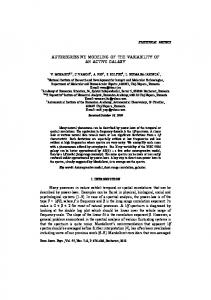
In this section, we will use the various models for ozone forecasting, and compare the predictions on our real data set. We developed one specific library in the statistical software R (see Ihaka and Gentleman (1996)), which might be soon submitted to the CRAN (cran.r-project.org). Since we noticed that our series were not stationary, we decided as usual to remove trend and seasonality. Of course, the daily seasonality is kept, because functional models can cope with it. We only dropped the annual trend and seasonality. We observed a relatively large heteroscedasticity over a year, but since we focused our study on summers, this problem disappeared. The ozone data we studied, during the period from 1995 to 1999, are distributed as shown in figure 1. The annual means of the series considered are presented in table 1.

1995 1996 1997 1998 1999

Ozone (µg/m3 ) 29 26 31 36 36

Temperature (◦ C) 12 9.1 12 12 13

Wind speed (m/s) 4.7 4.1 4 4.3 4.2

Table 1: Trend of the series computed as annual means Thinking that modelling the trend with such a small sample with unequally distributed missing values may be hazardous, we simply report the 1999 estimated trends for year 2000. We are comforted in our choice by the lack of a clear evolution in table 1. To evaluate the seasonality of ozone, temperature and wind speed series, we performed a simple Nadaraya-Watson regression of the series on the time, with a cross-validation procedure leading to a bandwidth of 25 days. Figure 2 present the smoothed seasonalities we obtained. It may be observed that the wind speed seasonality is not really significative compared to the observed levels. 8

Daily maximum ozone concentration

200 150 0

0

1000

50

100

days

3000

hours

5000

250

Hourly ozone concentration

0

50

100

150

200

0

50

100

O3 (µg m3)

150

200

O3 (µg m3)

Figure 1: Ozone concentrations

Seasonality of the temperature series

Seasonality of the wind speed series

0.0

(WS − WS) (m s)

−0.5

−5

0

(Tem − Tem) (°C)

0 −5 −10 −15

(O3 − O3) (µg m3)

5

0.5

5

10

Seasonality of the ozone series

0

100

200 day of the year

300

0

100

200

300

day of the year

Figure 2: Centered seasonalities

9

0

100

200 day of the year

300

We focused on the summer period for data, both in estimation and forecast procedures. Indeed, because of higher values of ozone, authorities are more interested in summer study. This choice is also relevant for modelling , and corresponds to our previous remarks on heteroscedasticity. We may mention that with this selection in the data, the forecasts were slightly better in the summer merely because of better fitted data, but overall criteria were higher since the ozone concentrations - and consequently the possible errors - are much lower in the winter. Our period of interest was from day 120 to day 270 in the year, which makes 151 days and not exactly a summer. The predictions were only available on 77 days, of which 6 days could not be used for comparison purposes, because of missing values. The mean value of ozone during summer 2000 was approximately 81 µg/m3 .

3.1

Estimation

In order to tune the various models well, we chose to perform cross-validation procedures on summer 1999, that is a fifth of the training data set. • For the functional kernel, the optimal bandwidth was 105 for L2 errors. This high number explains the smoothness of the prediction for this model. Maybe a L∞ cross-validation would have provided a different behavior. • For the ARH model, the procedure led to kn = 12 for L1 , L2 and L∞ errors as shown in table 2. • Concerning the ARHX(a) model, the cross-validation procedure led to kn = 35 for L2 and L∞ errors (and kn = 36 for L1 errors). It may seem large, but is relatively fitted to the size of the model (72 components because of 3 variables). • The ARHX(b) model was the hardest model to fit, because of the high combinatorial choice of the parameters (243 = 13824 choices). Nevertheless, the computation yielded   kn(1) , kn(2) , kn(3) = (7, 8, 7) where the variables are respectively ozone, temperature and wind speed. Figure 3 (1) shows how the L2 norm is disrupted when kn = 7 and the other parameters vary.

Although the ARH model is not parametric, one may give interpretations of the eigenvectors associated to the first eigenvalues and the coefficients of ρˆn . For example we can guess in figure 4 that the mean daily seasonality is in the space spanned by the eigenvector associated to the first eigenvalue. It should be interesting to link those informations to the chemical processes involved in ozone evolution.

10

kn 1 2 3 4 5 6 7 8 9 10 11 12

L1 norm 18.603 17.873 17.075 16.407 16.223 16.101 15.921 15.835 15.791 15.743 15.732 15.711

L2 norm 21.645 20.975 20.262 19.648 19.446 19.324 19.206 19.186 19.152 19.113 19.078 19.047

L∞ norm 39.851 39.491 38.621 38.021 37.611 37.435 37.412 37.319 37.347 37.282 37.18 37.147

kn 13 14 15 16 17 18 19 20 21 22 23 24

L1 norm 15.774 15.748 15.758 15.725 15.754 15.741 15.778 15.847 15.858 15.774 15.92 15.925

L2 norm 19.119 19.114 19.131 19.105 19.148 19.128 19.163 19.249 19.258 19.132 19.296 19.326

L∞ norm 37.313 37.354 37.429 37.456 37.610 37.541 37.67 37.704 37.758 37.529 37.821 37.898

Table 2: Cross-validation for the ARH model

3.2

Comparison

The various models aim at assessing the dynamics of ozone creation or dispersion. In figure 5, it is possible to see that the two ARHX models are relatively good for that purpose: the increase of July 24th and the decrease the next day are relatively well predicted, as well as the stability during September 16. The prediction of the high level of August 24th is only slightly underestimated, and the exit of the high ozone episode the next day is well predicted. We are a little bit disappointed with the behavior of ARHX models during August 23rd, which might be explained by a lack of meteorological variables. In terms of functional criteria for measuring the accuracy of the forecasts, the table 3 shows that the modifications suggested to improve the ARHX model in its ARHX(b) version is relevant. Figure 6 illustrates the daily behavior of L2 errors.

L1

norm norm L∞ norm L2

ARH 14.29 17.73 35.5

ARHX(a) 13.23 15.86 32.15

ARHX(b) 12.79 15.45 30.88

Kernel 16.37 19.75 38.94

Table 3: Mean functional errors of the models during summer 2000 Some ozone standards are calculated upon the daily maximum. Therefore, we used this complementary approach to compare the behavior of the predictions. The Generalized Additive Models (GAM) - see Hastie and Tibshirani (1990) - appeared to be very competitive in forecasting the peaks in ozone as shown in Davis and Speeckman (1999). That is why we decided to add two new alternative models, already discussed in this context,

11

L2 norm with kn(1) = 7 18.5

20

18.0

17.5

kn

3

15

17.0 10 16.5 5 16.0

5

10

15

20

(2)

kn

Figure 3: Levels of the L2 error with varying parameters for temperature and wind speed denoted respectively by GAM 1 and GAM 2 and defined roughly by O3 max = f1 (O3 max lag1 ) + f2 (T max) + f3 (Wmean)

(6)

log (O3 max) = g1 (O3 max lag1 ) + g2 (T max) + g3 (Wmean)

(7)

where: • O3 max stands for the daily maximum of ozone, • O3 maxlag1 stands for the daily maximum of ozone tha day before, • Tmax stands for the daily maximum of temperature, • Wmean stands for the daily mean of wind speed, • and f1 , f2 , f3 , g1 , g2 and g3 are unspecified functions to be estimated by the GAM procedure. Although ARHX models do not aim at forecast curves maxima, they showed good predictive skills in this field, outperforming the other functional models as seen in table 4. The two versions of the ARHX model reveal somehow different qualities: the (a) version 12

First eigenvectors for the ARH(1) v3 v4

−0.2

−0.1

0.0

0.1

0.2

0.3

0.4

v1 v2

0

5

10

15

20

time

Figure 4: First four functional eigenvectors of the covariance operator in the ARH(1) model

performs better for predicting the daily maximum, and the (b) version performs better for predicting the entire daily curve. Besides, the RMSE is lower for the ARHX(a) than for the GAM models. The MAE, MRE and MRAE are lower for the GAM models. Figure 7 illustrates the daily behavior of each model for predicting the daily maximum.

ARH ARHX(a) ARHX(b) Kernel GAM1 GAM2

MSE 445.6 239.4 275.4 527.6 249.2 274

RMSE 21.11 15.47 16.59 22.97 15.78 16.55

MAE 16.62 12.89 13.55 16.56 11.80 12.59

MRE -0.04828 -0.02443 -0.04191 -0.0353 0.04587 0.0104

MRAE 0.2092 0.1702 0.1751 0.2034 0.1655 0.1694

Table 4: Errors on the daily maximum of the various models during summer 2000 Another point of view is to consider the distribution of errors in terms of classes. Firstly, if we look at 10 µg/m3 long intervals, we obtain table 5. Secondly, if we look at error in term of the number of classes in the so-called ATMO index for ozone, we obtain table 6. Let us recall before what are the ATMO classes for daily maximum of ozone in µg/m3 : [0, 30[ , [30, 55[ , [55, 80[ , [80, 105[ , [105, 130[ , [130, 150[ , [150, 180[ , [180, 250[ , [250, 360[ , [360, ∞[ . The success rate of ATMO index prediction is computed as the number of 0 an 1 class error divided by the number of predictions.

13

0

5

10

15

20

100 50

0

5

10

15

20

15

20

100

10

15

20

15

20

100

10

15

20

0

5

10

20

15

20

150

16/09/00

100

observations ARH ARHX(a) ARHX(b) Kernel

0

50

100

observations ARH ARHX(a) ARHX(b) Kernel

50

20

15

150

5

0

15

20

50

0

150

150 100 50 0

10

10

observations ARH ARHX(a) ARHX(b) Kernel

15/09/00

observations ARH ARHX(a) ARHX(b) Kernel

5

5

0

50

100

observations ARH ARHX(a) ARHX(b) Kernel

14/09/00

0

0

25/08/00

0

10

15

50

5

150

150 100 50

5

20

observations ARH ARHX(a) ARHX(b) Kernel

24/08/00

0

0

15

0

0

23/08/00 observations ARH ARHX(a) ARHX(b) Kernel

10

150

150 100

observations ARH ARHX(a) ARHX(b) Kernel

50

10

5

31/07/00

0

0

50

100

observations ARH ARHX(a) ARHX(b) Kernel

5

0

30/07/00

150

29/07/00

0

observations ARH ARHX(a) ARHX(b) Kernel

0

50

100

observations ARH ARHX(a) ARHX(b) Kernel

0

0

50

100

observations ARH ARHX(a) ARHX(b) Kernel

150

25/07/00

150

24/07/00

150

23/07/00

0

5

10

15

20

0

5

10

Figure 5: Comparison of the various model for predicting ozone (in µg/m3 )

14

40

Comparison of the daily L2 errors of the models

30 25 20 10

15

L2 daily errors

35

ARH ARHX(a) ARHX(b) Kernel

0

10

20

30

40

50

60

70

days

Figure 6: Comparison of L2 errors of the various model during summer 2000 (missing values are excluded)

Comparison of the daily maximum obtained by the different models

120 100 80 60 40

Daily ozone maximum

140

observations ARH ARHX(a) ARHX(b) Kernel GAM1 GAM2

0

10

20

30

40

50

60

70

days

Figure 7: Comparison of predicted daily maxima of ozone versus real ones of the various model during summer 2000 (missing values are excluded)

15

[0;10] ]10;20] ]20;30] >30

ARH 42.25 % 21.13 % 22.54 % 14.08 %

ARHX(a) 39.44 % 39.44 % 15.49 % 5.634 %

ARHX(b) 45.07 % 28.17 % 23.94 % 2.817 %

Kernel 40.85 % 28.17 % 15.49 % 15.49 %

GAM1 46.48 % 35.21 % 14.08 % 4.225 %

GAM2 49.3 % 32.39 % 12.68 % 5.634 %

Table 5: Classes of errors for the maximum of the day during summer 2000

0 class 1 class 2 classes 3 classes Success Rate

ARH 28 35 7 1 88.73 %

ARHX(a) 31 38 2 0 97.18 %

ARHX(b) 34 35 2 0 97.18 %

Kernel 33 30 5 3 88.73 %

GAM1 35 33 2 1 95.77 %

GAM2 34 33 3 1 94.37 %

Table 6: Errors on the ozone ATMO index during summer 2000

4

Conclusion

The ozone forecasting problem is both a health issue and a difficult problem. The statistical methods presented above show good skills for this purpose. The functional approach seems relevant. The autoregressive Hilbertian model with exogenous variables in its two version was the best model with respect to functional or daily maximum criteria. Several improvements should be developed. The first are methodological ones. Indeed, in the pollution field, practicians are interested in specific hours and horizons of prediction, for instance in the afternoon of the day before in order to inform the population better, or in the morning of the day considered in order to increase the accuracy of the forecasts. Accordingly, modifications of our model are necessary to cope with such a problematic by considering overlapping intervals for example. Furthermore, since peaks are not easy to predict, the methodology could change slightly for that purpose by putting weights on highly polluted days during the estimation procedure. The second are practical. It seems clearly interesting to take into account more information about the meteorological situation or human activities. Hence, exogenous variables such as solar radiation, humidity, precipitation, pressure, cloud cover and day of the week should be inputs of the model. Those variables are not always easy to measure or predict, and a careful use has to be made. Acknowledgement: We are grateful to the AREMARTOIS association for supplying the data.

References Barrat M, Lecluse Y, Slamani Y. 1990. Etude comparative de diff´erents mod`eles math´ematiques pour la pr´ediction des niveaux de pollution atmosph´erique, analyse uni-

16

variable. R.A.I.R.O. APII 3: 283–298. Bauer G, Deistler M, Scherrer W. 2001. Time series models for short term forecasting of ozone in the eastern part of Austria. Environmetrics 12: 117–130. Besse P, Cardot H. 1996. Approximation spline de la pr´evision d’un processus fonctionnel autor´egressif d’ordre 1. Revue Canadienne de la Statistique/Canadian Journal of Statistics 24: 467–487. Besse P, Cardot H, Stephenson D. 2000. Autoregressive forecasting of some functional climatic variations. Scandinavian Journal of Statistics 27(4): 673–687. Bosq D. 2000. Linear Processes in Function Spaces : Theory and Applications, volume 149 of Lecture Notes in Statistics. Springer-Verlag, New York. Boznar M, Lesjak M, Mlakar P. 1993. A neural network-based method for short-term predictions of ambient SO2 concentrations in highly polluted industrial areas of complex terrain. Atmospheric Environnement 27B(2): 221–230. Breiman L, Friedman J, Ohlsen R, Stone R. 1984. Classification and regression trees. Belmont, CA, Wadsworth. Comrie A C, Diem J E. 1999. Climatology and forecast modeling of ambient carbon monoxide in phoenix, arizona. Atmospheric Environnement 33: 5023–5036. Davis JM, Speeckman P. 1999. A model for predicting maximum and 8 h average ozone in houston. Atmospheric Environment 33: 2487–2500. Gardner MW, Dorling SR. 1999. Neural network modelling and prediction of hourly NOx and NO2 concetrations in urban air in london. Atmospheric Environnement 33: 709–719. Gardner MW, Dorling SR. 2000. Statistical surface ozone models: an improved methodology to account for non-linear behaviour. Atmospheric Environnement 34: 21–34. Ghattas B. 1999. Pr´evisions des pics d’ozone par arbres de r´egression simples et agr´eg´es par bootstrap. Revue de Statistique Appliqu´ee XLVII(2). Gonzalez-Manteiga W, Prada-Sanchez JM, Cao R, Garcia-Jurado I, Febrero-Bande M, Lucas-Domingez T. 1993. Time series analysis for ambient concentrations. Atmospheric Environnement 27A(2): 153–158. Graf-Jacottet M, Jaunin M-H. 1998. Predictive models for ground ozone and nitrogen dioxide time series. Environmetrics 9: 393–406. Guillas S. 2000. Non-causalit´e et discr´etisation fonctionnelle, th´eor`emes limites pour un processus ARHX(1). C. R. Acad. Sci. Paris S´er. I Math. 331: 91–94. Hastie TJ, Tibshirani RJ. 1990. Generalized additive models. Chapman & Hall, New-York. 17

Ihaka R, Gentleman R. 1996. R: A language for data analysis and graphics. Journal of Graphical and Computational Statistics 5: 299–314. Kocak K, Saylan L, Sen O. 2000. Nonlinear time series prediction of O3 concentration in istanbul. Atmospheric Environnement 34: 1267–1271. M´elard G, Roy R. 1988. Mod`eles de s´eries chronologiques avec seuils. Revue de Statistique appliqu´ee XXXVI(4): 5–24. Mourid T, 1995. Contribution ` a la statistique des processus autor´egressifs ` a temps continu. D. sc. thesis, Universit´e Paris 6. Nadaraja E A. 1964. On estimating regression. Theory Probab. An. pages 141–142. P´erez P, Trier A, Reyes J. 2000. Prediction of PM2.5 concentrations several hours in advance using neural networks in santiago, chile. Atmospheric Environnement 34: 1189–1196. Pitard A, Viel JF. 1999. A model selection tool in multi-pollutant time series: The Granger-causality diagnosis. Environmetrics 10: 53–65. Prada-Sanchez JM, Febrero-Bande M, Cotos-Yanez T, Gonzalez-Manteiga W, BermudezCela L, Lucas-Domingez T. 2000. Prediction of SO2 pollution incident near a power station using partially linear models and an historical matrix of predictor-response vectors. Environmetrics 11: 209–225. Ramsay J, Silverman B. 1997. Functional Data Analysis. Springer-Verlag. Rice J, Wu C. 2001. Nonparametric mixed effects models for unequally sampled noisy curves. Biometrics 57: 253–259. Ruiz-Suarez JC, Mayora-Ibarra OA, Torres-Jimenez J, Ruiz-Suarez LG. 1995. Short-term ozone forecasting by artificial neural networks. Advances in Engineering Software 23: 143–149. Silvia C, P´erez P, Trier A. 2001. Statistical modelling and prediction of atmospheric pollution by particulate material: two nonparametric approaches. Environmetrics 12: 147–149. Watson G S. 1964. Smooth regression analysis. Sankhya Ser. A 26: 359–372. Yi J, Prybutok VR. 1996. A neural network model forecasting for prediction of daily maximum ozone concentration in an industrialized urban area. Environnemental Pollution 3: 349–357.

18

LISTE DES RAPPORTS TECHNIQUES

N◦ 1

F´evrier 1999

Autoregressive Hilbertian Process Denis BOSQ

N◦ 2

Avril 1999

Using the Entringer numbers to count the alternating permutations according a new parameter Christiane POUPARD

N◦ 1

Mars 2000

Noncausality and functional discretization, limit theorems for an ARHX(1) process Serge GUILLAS

N◦ 2

Juin 2000

Sieve estimates via neural network for strong mixing processes Jian tong ZHANG

N◦ 3

Juillet 2000

Technical tools to evaluate Hausdorff-Besicovitch measure of random fractal sets Alain LUCAS

N◦ 1

Avril 2001

Rates of convergence of autocorrelation estimates for autoregressive Hilbertian processes Serge GUILLAS

N◦ 2

Avril 2001

Sur l’estimation de la densit´e marginale d’un processus ` a temps continu par projection orthogonale Arnaud FRENAY

N◦ 3

Juin 2001

Rate-optimal data-driven specification testing in regression models Emmanuel GUERRE et Pascal LAVERGNE

N◦ 4

Juin 2001

The inclusion of exogenous variables in functional autoregressive ozone forecasting Julien DAMON et Serge GUILLAS

20