Sep 22, 2016 - ity, but are expected to effectively damp away constraint violation in numerical ..... urally a proof of numerical stability is desirable, at least.
The initial boundary value problem for free-evolution formulations of General Relativity David Hilditch1 and Milton Ruiz2,3,4 1
arXiv:1609.06925v1 [gr-qc] 22 Sep 2016
Theoretical Physics Institute, University of Jena, 07743 Jena, Germany 2 Department of Physics, University of Illinois at Urbana-Champaign, Urbana, IL 61801 3 Escuela de F´ısica, Universidad Industrial de Santander, Ciudad Universitaria, Bucaramanga 680002, Colombia 4 Departament de F´ısica, Universitat de les Illes Balears, Palma de Mallorca, E-07122, Spain We consider the initial boundary value problem for free-evolution formulations of general relativity coupled to a parametrized family of coordinate conditions that includes both the moving puncture and harmonic gauges. We concentrate primarily on boundaries that are geometrically determined by the outermost normal observer to spacelike slices of the foliation. We present high-order-derivative boundary conditions for the gauge, constraint violating and gravitational wave degrees of freedom of the formulation. Second order derivative boundary conditions are presented in terms of the conformal variables used in numerical relativity simulations. Using Kreiss-Agranovich-M´etivier theory we demonstrate, in the frozen coefficient approximation, that with sufficiently high order derivative boundary conditions the initial boundary value problem can be rendered boundary stable. The precise number of derivatives required depends on the gauge. For a choice of the gauge condition that renders the system strongly hyperbolic of constant multiplicity, well-posedness of the initial boundary value problem follows in this approximation. Taking into account the theory of pseudodifferential operators, it is expected that the nonlinear problem is also well-posed locally in time.
I.
CONTENTS
I. Introduction II. Formulation of the IBVP A. Analytical Setup B. Boundary conditions C. Conformal decomposition D. Second order boundary conditions on the conformal variables III. Well-posedness analysis A. Basic strategy B. Strong hyperbolicity and multiplicity of speeds C. Kreiss-Agranovich-M´etivier Theory D. Laplace-Fourier transformed system E. L2 solution of the reduction F. Laplace-Fourier transformed boundary conditions with the boundary orthogonality condition G. Well-posedness results using fifth order BCs, the boundary orthogonality condition and general gauges H. Why work under the boundary orthogonality condition? IV. Conclusion
1 2 2 4 6 7 8 8 8 9 10 11
14
16 18 18
Acknowledgments
19
References
19
INTRODUCTION
For standard applications in numerical relativity we are forced to consider the mathematical properties of the initial boundary value problem (IBVP) for general relativity. An essential property of the IBVP is that it should be well-posed. The requirement of well-posedness is three-fold. We require that a solution exists, is unique, and depends continuously on given initial and boundary data [1, 2]. There are further complications. Formulations of general relativity (GR) typically have constraints which must be satisfied in order to recover a full solution of the Einstein equations. If the boundary conditions (BCs) are not constraint preserving then, even if the IBVP is wellposed, as illustrated for example in [3–5], constraint violations will enter through the boundary and render the solution of the partial differential equation (PDE) system unphysical. Furthermore, since we are often interested in solutions that are asymptotically flat, we would like the BCs to be as transparent as possible to outgoing radiation, be it physical or gauge, in the sense that these conditions do not introduce large spurious reflections from the boundary. Such reflections would either be unphysical, or simply produce undesirable gauge dynamics. A general discussion of non-reflecting BCs of the wave problem in applied mathematics and engineering can be found in [6]. Two formulations of GR are currently known to admit a well-posed IBVP with constraint preserving boundary conditions (CPBCs) [7–12]. They are the generalized harmonic gauge (GHG) [13–15] and Friedrich-Nagy formulations [7]. Of these, GHG has been used widely in numerical relativity simulations [16– 20]. Boundary conditions employed in GHG numerical simulations are described, for instance, in [9, 21, 22].
2 On the other hand, many numerical relativity groups use formulations involving a conformal decomposition of the field equations, such as the Baumgarte-Shapiro-ShibataNakamura-Oohara-Kojima (BSSNOK) formulation [23– 25] or a conformal decomposition of the Z4 formulation [26, 27] as developed in [5, 28–32]. These formulations are normally used in combination with the moving puncture gauge condition [33–38]. The IBVP for these ‘conformal’ formulations is less well understood. The key difficulty, as we shall see, is the complicated structure of the principal part of the equations with the moving puncture gauge. Thus most codes use so-called radiative boundary conditions on every evolved field [39], which overdetermine the IBVP and therefore are expected to render it ill-posed. These conditions do not preserve the constraints. Well-posedness of the IBVP of BSSNOK has been studied in a number of places. For instance, in [40] the dynamical BSSNOK system is recast as a first order symmetric hyperbolic system and the corresponding IBVP shown to be wellposed through a standard energy method. However, the boundary conditions presented in [40] do not preserve the constraints, and the analysis of the IBVP does not include the moving puncture gauge condition. In [41] constraint preserving boundary conditions for the BSSNOK formulation were shown to give a well-posed IBVP when the system is linearized around flat-space. These conditions have not yet been tested in numerical relativity simulations. A numerical implementation of CPBCs in spherical symmetry for the above system were presented in Appendix B of [42], and extensively tested in [43]. The key point of this implementation is to numerically construct the outgoing and incoming modes, and to express the latter in terms of the constraints where possible. BCs are then set to enforce that the incoming modes do not introduce spurious reflections. For a detailed discussion of the IBVP in GR, see the review [44]. For the Z4 formulation CPBCs are straightforward, since the constraint subsystem consists entirely of wave equations, whereas the BSSNOK constraint subsystem contains a characteristic variable with vanishing speed. Using this fact, CPBCs were implemented, in explicit spherical symmetry, and shown very effective at absorbing constraint violations [5]. Moreover BCs compatible with the constraints for a symmetric hyperbolic first order reduction of Z4 were specified and studied in numerical applications in [45, 46]. The conditions are of the maximally dissipative type and so well-posedness of the resulting IBVP could be shown with a standard energy estimation, although harmonic slicing and normal, or vanishing shift, coordinates were employed, and it is not clear how generally the results can be extended to other gauge choices. Full 3D numerical relativity simulations using Z4c and radiation controlling, CPBCs were presented [47]. But no attempt was made to analyze well-posedness of the IBVP. In this work, we therefore attempt to complete the theoretical story, in the sense that we prove well-posedness
of the IBVP, in the frozen coefficient approximation, of particular formulations of GR coupled to a parametrized family of gauge conditions including both the harmonic and moving puncture gauges. Our discussion will focus primarily on the formulation of [48]. From the PDEs point of view this is the preferred choice of formulation because it decouples the gauge and constraint violating degrees of freedom to the greatest degree possible for the live gauges under consideration. This formulation has not yet been used in numerical relativity but is expected to have all of the advantages of Z4 over BSSNOK, most notably propagating constraints, whilst simultaneously avoiding possible breakdown of hyperbolicity associated with the clash of gauge and constraint violating characteristic speeds. The Mathematica notebooks that accompany the paper can be easily modified to treat the Z4 and BSSNOK formulations. By the theory of pseudodifferential operators, our calculations are expected to extend locally in time to the original nonlinear equations [2, 49]. We begin in section II with a summary of the formulation, a geometric formulation of the problem and the identification of the BCs taken in the subsequent analysis. Our geometric formulation fixes the outer boundary to be that timelike surface generated by the outermost observers in the initial data as they are Lie-dragged up the foliation by the timelike normal vector. This results in an outer boundary that may drift in local coordinates. The numerical relativist interested in implementing a basic approximation to our conditions need only concern themselves with sections II C and II D. Section III contains our well-posedness results with high order BCs, and discussion of the difficulties that arise if we try to fix the coordinate position of the outer boundary, plus gauge conditions in which this is straightforward, and in which the fewer derivatives are required to achieve boundary stability. We conclude in section IV.
II.
FORMULATION OF THE IBVP
In this section, we summarize the geometrical setup of the IBVP, present the formulation of [48] in the ADM and conformal variables and discuss the high-order BCs analyzed in section III. Finally, we display the second order special case of the BCs in terms of the conformal variables that are used in standard numerical applications. Here ‘order’ refers to the highest derivative of either the metric, lapse or shift components appearing in the boundary condition.
A.
Analytical Setup
Manifold structure and geometry of the boundary: We investigate the evolution equations on a manifold M = [0, T ]×Σ. The three dimensional compact manifold Σ has smooth boundary ∂Σ. We assume that the gravitational
3
na
St +Δt
la sa
St
we say that we work “under the boundary orthogonality condition”. Notice that this leads to a hyperbolic equation of motion,
Σt +Δt
∂t (∂i r) = β j ∂j (∂i r) + (∂j r)∂i β j ,
Σt
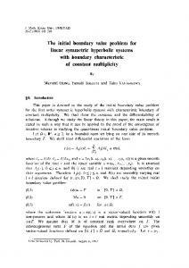
FIG. 1. Manifold setup for the IBVP. The manifold is foliated by three dimensional surfaces Σt . We impose a timelike boundary condition St in a compact region of each surface Σt , which restricts the domain of dependence of the initial data to the inner conical region of the timelike tube T .
field is weak near the boundary so that the boundary of the full manifold T = [0, T ] × ∂Σ is timelike and the three dimensional slices Σt = {t} × Σ are spacelike as shown in Figure 1. The boundary of a spatial slice is denoted St = {t} × ∂Σ. We define na , the future pointing unit normal to the slices Σt , and similarly employ the standard notation for the induced metric γab and intrinsic curvature Kab of the foliation. The spatial covariant derivative is denoted D. Initial data will be specified on some constant t slice, and boundary conditions, yet to be determined, on T . The outer boundary T can be characterized as the level set of a scalar field r = rB , defined at least in a neighborhood of T . We may then perform a 2 + 1 split relative to the unit spatial vector, sa = LDa r ,
(1)
where we define the length scalar L−2 = γ ab Da rDb r, to study the geometry of the boundary. We will however only introduce the quantities to be employed in the boundary conditions. The vector sa is thus the unit normal to the two-surface {t} × ∂Σ as embedded in Σt . The standard approach in numerical relativity is to take r to be a radial-type coordinate built in the normal way from the asymptotically Cartesian coordinates defining the tensor basis used to represent the evolved variables. In this case we have ∂t r = 0 and so the coordinate position of the outer boundary is fixed in time. Perhaps a more geometrically natural condition is to insist that the future pointing normal na to slices of the foliation point directly up the boundary. This can be achieved by requiring instead Ln r = 0, which must be solved at least in a neighborhood of the outer boundary. One may then think of r as a natural radial coordinate of normal observers to the slice. When working under this assumption
(2)
for the appropriate components of the Jacobian mapping between the two coordinate systems, since the second term is non-principal, as it may be replaced by a firstorder reduction variable in any such reduction. The numerical implementation of this idea is left to future work, but we note that the approach fits naturally within the dual foliation formalism [50]. A consequence of insisting on working with the boundary orthogonality condition is that the outer boundary will drift in local coordinates. Geometrically this condition is the same as that for the longitudinal component of the shift in [41] for BSSNOK. But now r is not one of our coordinates, and nor is the ∂ a associated vector ( ∂r ) necessarily a member of the tensor basis in which we work for the 3 + 1 evolution. The motivation for choosing this orthonormality in the BSSNOK case was that in this way the number of incoming characteristic fields at the outer boundary can be fixed, removing the need to treat various special cases. With the present formulation that motivation is absent because there are no shift-speed characteristic variables. This imposes a major difference in our analysis as compared to the standard boundary treatment in numerical relativity, where the outer boundary remains at fixed coordinates. We expect that this complication can be sidestepped by working with the dual-foliation formalism, but this will be investigated elsewhere. The problems that arise in the PDEs analysis if we do not work with the boundary orthogonality condition are discussed in section III H. Newman-Penrose null tetrad: The previous vector fields allow us to introduce, for later convenience, the following Newman-Penrose null vectors, 1 1 la = √ (na + sa ) , k a = √ (na − sa ) , 2 2 1 1 a a a a m = √ (ι + i υ ) , m ¯ = √ (ιa − i υ a ) , 2 2
(3)
where ιa and υ a are spatial unit vectors mutually orthogonal to both na , sa and each other. Equations of motion: Following [48], in which the formulation was first presented, we replace the Einstein equations with the expanded set of equations, ∂t γij = −2αKij + Lβ γij , ∂t Kij = −Di Dj α + α[Rij − 2Ki k Kkj + KKij ˆ (i Zj) − κ1 (1 + κ2 )γij Θ] + 2D + 4πα[γij (S − ρ) − 2Sij ] + Lβ Kij ,
(4)
where Θ and Zi are a set of four variables defining an expanded phase space in which our PDEs analysis is performed, and we must have Θ = Zi = 0 to recover solutions of GR. The equations of motion for these variables
4 are given momentarily. We write, ˆ i Zj ≡ γ − 31 γkj ∂i Z˜ k , D
1 Z˜ i = γ 3 Z i .
(5)
The free parameters κ1 and κ2 serve to parametrize the strength of constraint damping in the evolution equations [51]. These terms were not included in the discussion of [48] and, as non-principal terms will play no fundamental role in the discussion of boundary stability, but are expected to effectively damp away constraint violation in numerical applications. Here we also modify the constraint addition as compared with [48] so that the equations of motion look as natural as possible when written in terms of the conformal variables. The dynamical ADM equations are of course recovered when the constraints Θ and Zi vanish. Constraints: The set of constraints Θ, Zi are completed by the Hamiltonian and momentum constraints, H ≡ R − Kij K ij + K 2 − 16πρ = 0 ,
ˆ = K −2 Θ, the contracted conformal Christoffel where K is a shorthand for, h i ˜ i = γ 13 γ ij 2 Zj + γ kl (∂k γlj − 1 ∂j γkl ) , Γ (11) 3 and the conformal metric is defined by γ˜ij = χ γij , with χ = γ −1/3 . The harmonic gauge is recovered with the choice µL = ηχ = 1, µS = ηL = 1, and η = 0. The standard moving puncture gauge choice is the “1+log” variant of the Bona-Mass´o condition, µL = 2/α, combined with the Gamma-driver shift [53], with ηχ = ηL = 0, and various choices for µS . The effect of the gauge damping term η on numerical simulations with the Gamma-driver shift has been studied in [54–56]. Projection operators: We define the projection operators into directions tangential to the boundary St , and onto the “physical” degrees of freedom by, q i j = δ i j − si sj ,
Mi ≡ Dj (Kij − γij K) − 8πSi = 0 .
(6)
1 q (P )ij kl = q i (k q j l) − qkl q ij , (12) 2
respectively. We use the notation, Their equations of motion are, � � 1 i ˆ ∂t Θ = α H + D Zi − κ1 (2 + κ2 )Θ + Lβ Θ , 2 � � � 1 4 − ηχ Di Θ − κ1 Zi ∂t Zi = α Mi + 3 h i 1 1 ˆ j Zi , + γ 3 Z j ∂t γ − 3 γij + β j D (7) where the scalar ηχ is determined by the gauge choice as discussed below. The time dependence of the constraints can be computed from (4), and is found to be, ∂t H = − 2αDi Mi − 4 Mi Di α + 2 α K H � ˆ (i Zj) + 2 α 2 K γ ij − K ij D
DA DB α ≡ q i A q j B Di Dj α ,
(14)
where we use upper case Latin letters to denote indices that have been projected into the directions tangential to St . Boundary conditions
(8) We want to impose BCs on the formulation. Following [9, 57], these conditions should satisfy the following conditions:
for the Hamiltonian constraint and 1 ∂t Mi = − αDi H + α K Mi − (Di α) H 2 � � � � ˆ (k Zl) ˆ (i Zj) − Di 2 α γ kl D + Dj 2 α D (9)
for the momentum constraint. It is clear that this formulation is a mild modification of the Z4c system, the only difference in the principal part occurring in (7). Gauge conditions: We close the evolution system with a parametrized gauge condition, consisting of the Bona-Mass´ o lapse condition [52] and the shift condition, ˆ + β i ∂i α , ∂t α = −α2 µL K h i ˜ i + 1 ηχ γ˜ ij ∂j ln χ − α ηL χ γ˜ ij ∂j α ∂t β i = α2 µS χ Γ 2 − η β i + β j ∂j β i ,
(13)
for longitudinal derivatives; we do not commute the spatial normal vector with any derivative operator. Likewise, we never commute the projection operator with any derivative operator, so for example,
B.
− 4 κ1 (1 + κ2 ) α K Θ + Lβ H ,
+ 2κ1 (1 + κ2 ) Di (α Θ) + Lβ Mi ,
Ds Ds α ≡ si sj Di Dj α ,
(10)
Well-posedness: The IBVP must be well-posed. Without this requirement, existence of a solution, even locally in time, is not guaranteed. Without continuous dependence on given data at the continuum level, no numerical method can converge to the continuum solution. Furthermore, in principle without continuous dependence the PDE formulation of the physical problem has no predictive power. Constraint preservation: The conditions should be constraint preserving. Otherwise the physical solution will be compromised as soon as it is reached by the constraint violations propagating from the outer boundary into the domain. Radiation control: The BCs should minimize spurious reflections and allow us to control the incoming
5 gravitational radiation. Without this property, the solution can not necessarily be viewed as an isolated body unperturbed by incoming waves. Note that this characterization relies on the assumption that the gravitational field near the boundary is weak. With these considerations in mind, we propose the following set of BCs: Gauge boundary conditions: Following [5], for the lapse we choose the boundary condition, �
r2 iaµL ∂a
�L+1
α= ˆ (r2 Ln )L+1 hL ,
(15)
where iaµL the vector pointing along the outgoing characteristic surfaces of the Bona-Mass´ o lapse condition, defined according to, � 1 √ iaµ = √ na + µ sa , 2
(16)
a shorthand valid for arbitrary µ > 0, and Ln the derivative along the na direction. Here, and in what follows, = ˆ denotes an equality which holds only in the boundary St . We take L to be a natural number, and hL an arbitrary smooth scalar function in the boundary which can be interpreted as the given boundary data. Next, in order to specify BCs on the components β i , define the shorthands µSL = (4 − ηχ ) µS /3 and, � � η µ −µ ˆ . (17) B s = iaµS ∂a (∂i β i ) − LµLL−µS SL α iaµS ∂a K L
L
L
We emphasize that this variable has nothing to do with the standard reduction variable “B i ” used sometimes with the moving-puncture gauge. The reason for choosing this particular combination will become clear during the following analysis. We choose the BC, r
4
�
r2 iaµS ∂a L
�L−1
s
2
L+1
B = ˆ (r Ln )
hSL ,
B A = γ ik s[k qj] A ∂i β j .
�L
� BA = ˆ (Ln )L−1 L2n − µS ∆ / hA µS .
(21)
where we have defined µC = µSL /µS = (4 − ηχ )/3 and choose given data hΘ which will be taken to vanish in applications. For the lowest derivative order L = 1 boundary we choose, ˜i , la ∂a Z˜ i = ˆ L2n h Z
(22)
˜ i = γ˜ ij hZ . This choice where we write Z˜ i = γ˜ ij Zj and h j Z is made so that the boundary conditions become more convenient when written in terms of the conformal variables used in numerical applications (see Sec. II C). For higher order conditions, however, it turns out to be more natural to make some adjustment. We use the shorthands, (23)
(18) The remaining constraint conditions are then,
(19)
For the transverse components of the shift we choose, r2 iaµS ∂a
�L � � �L+1 ˆ r2 Ln r2 r2 iaµC ∂a Θ = hΘ ,
˜ i = Ln Z˜ i − µC γ˜ ij Dj Θ . X
for the longitudinal component of the shift. The given data here is the scalar hβ s . Next we define the shorthand,
�
since we are also concerned with minimizing the number of derivatives in the conditions, we accept this potential shortcoming. We will see in the following analysis that the complicated characteristic structure of the gauge conditions forces us to take high order BCs (L = 4) so that we can obtain boundary stability in the analysis. The key point is to choose given data containing particular combinations of derivatives. To obtain boundary stability in the rest of the formulation we need only take L = 1. We can adjust the gauge so that there too, only L = 1 is required. For details see [58] and the Mathematica notebooks that accompany the paper. Constraint preserving boundary conditions: In [5], we studied high order BCs for the constraints Θ and Zi for the Z4c formulation. Here we are forced to modify those conditions because the characteristic structure of the constraint subsystem for the present formulation is slightly more complicated than that of Z4c. First for the scalar constraint Θ we choose,
(20)
The given data hA µS are to be treated as two smooth scalar functions in the boundary. The operator ∆ / is the two dimensional Laplacian associated with the induced metric qAB . The inclusion of this made in order to cancel bad terms in the following Laplace-Fourier analysis. Note that from the point of view of absorption of outgoing gauge waves this condition is not optimal, but
�
r2 la ∂a
�L−1
� i ˜ . ˜i = X ˆ (r2 Ln )L−1 L2n − ∆ / h Z
(24)
˜ i will typically be taken to vanAgain the given data h Z ish in applications, but we have to include it to show estimates in the free-evolution approach. Radiation controlling boundary conditions: A standard BC for the GHG formulation that controls the incoming gravitation radiation is the Ψ0 -freezing condition [7–9, 11, 12, 18, 57, 59, 60] which serves as a good first approximation to an absorbing condition [4, 61]. In particular, freezing Ψ0 to its initial value allows the absorption of outgoing gravitational waves by minimizing spurious reflections. It has been shown analytically [4] that the spurious reflections from the freezing-Ψ0 condition decay as fast as (k R)−4 , for monochromatic radiation with
6 wavenumber k and for an outer boundary with areal radius R. This condition has also been considered with the BSSNOK formulation [41]. To impose Ψ0 -freezing conditions, we take the electric and magnetic parts of the Weyl tensor [39], h iTF ˆ (i Zj) − 4 π Sij Eij = Rij + K Kij − K l i Kil + 2 D , Bij = �(i| kl Dk Kl|j) .
(25)
The Weyl scalar Ψ0 is given by, Ψ0 = (Emm − i Bmm ) ,
(26)
where the index m refers to contraction with the null vector ma . To motivate our choice of given data recall that, for linear plane gravitational waves propagating on flat space, we have [39] � 1 2 + ∂ h + 2∂t ∂r h+ + ∂r2 h+ 4 t � i − ∂t2 h× + 2∂t ∂r h× + ∂r2 h× , 4
Ψ0 = −
(27)
with h+ and h× the independent components of the transverse-traceless part of the metric perturbation. Assuming that we have an incoming gravitational wave, then h+ ∼ h× ∼ h(t + r) and then, Ψ0 = −∂t2 h+ − i ∂t2 h× .
(28)
Thus, for the lowest order boundary we choose, Ψ0 = ˆ (r2 Ln )2 hΨ0 ,
(29)
where hΨ0 is smooth given data at the boundary. For higher order BCs, One naively could hit the left-hand side of the above condition by a Sommerfeld boundary operator as many times as is desired. However since Ψ0 , depending on the particular gauge, satisfies in the principal part a wave equation only up to a coupling with Θ, the necessary analysis for arbitrary values of L becomes messy. To avoid this we choose, � �L−2 ˆ 0= r4 r2 la ∂a Ψ ˆ (r2 Ln )L+1 hΨ0 ,
(30)
ˆ 0 is given by for L ≥ 2, where the shorthand Ψ ˆ 0 = Ln Ψ0 − 2 µC Dm Dm Θ . Ψ
C.
Conformal decomposition
For numerical integration favorable PDE properties, such as well-posedness, may not be enough to guarantee robust evolution. It is therefore common to work with
conformally decomposed variables. We define the variables [28], 1
γ˜ij = γ − 3 γij ,
1
χ = γ− 3 ,
1 1 A˜ij = γ − 3 (Kij − γij K) , 3 ˜ i = 2 γ˜ ij Zj + γ˜ ij γ˜ kl ∂l γ˜jk , (Γ ˜ d )i = γ˜ jk Γ ˜ i jk , (31) Γ
ˆ = γ ij Kij − 2 Θ , K
the idea of which is to make as many variables as possible non-singular, so that for example puncture black holes can be treated numerically. Variations on this decomposition have been studied in the literature [62, 63], but here we will be satisfied with the vanilla form. Note ˜ i is compatible with the shortthat the definition of Γ hand given in (11). Under this change of variables the equations of motion become, i 2 h ˆ χ α (K + 2Θ) − Di β i , 3 ∂t γ˜ij = −2 α A˜ij + β k ∂k γ˜ij + 2 γ˜k(i ∂j) β k 2 − γ˜ij ∂k β k , 3 ∂t χ =
(32)
for the metric and, � � ˆ + 2Θ)2 ˆ = −Di Di α + α A˜ij A˜ij + 1 (K ∂t K 3 ˆ, + 4 π α [S + ρ ] + α κ1 (1 − κ2 ) Θ + β i ∂i K � �tf ∂t A˜ij = χ − Di Dj α + α (Rij − 8 π Sij ) h i ˆ + 2 Θ)A˜ij − 2 A˜k i A˜kj + α (K 2 + β k ∂k A˜ij + 2 A˜k(i ∂j) β k − A˜ij ∂k β k , 3
(33)
for the extrinsic curvature. For the contracted conformal Christoffels we have, � i ij ˜ i jk A˜jk − 3 A˜ij ∂j ln(χ) ˜ ˜ ∂t Γ = −2 A ∂j α + 2 α Γ 2 � 2 ij ˆ − 8 π γ˜ ij Sj + γ˜ jk ∂j ∂k β i − γ˜ ∂j K 3 1 ˜ i − (Γ ˜ d )j ∂j β i + γ˜ ij ∂j ∂k β k + β j ∂j Γ 3 � i � 2 ˜ i j ˜ ˜ i + (Γ (34) d ) ∂j β − 2 α κ1 Γ − (Γd ) . 3 The difference between Z4c and the present formulation, displayed in (7), propagates through the change of variables resulting in the disappearance of the Θ constraint from this equation. Finally we have, ∂t Θ =
� 1 � 2 ˆ α R − A˜ij A˜ij + (K + 2 Θ)2 2 � 3 � − α 8 π ρ + κ1 (2 + κ2 ) Θ + β i ∂i Θ .
(35)
This system can be trivially implemented in a moving puncture code as a modification of either the Z4c or
7 BSSNOK formulations. Within this decomposition the intrinsic curvature is written as, ˜ ij , Rij = Rχ ij + R ˜ χ ij = 1 D ˜ iD ˜ j χ + 1 γ˜ij D ˜ lD ˜ lχ R 2χ 2χ 3 1 ˜ ˜ ˜ l χD ˜ lχ , γ˜ij D − 2D i χDj χ − 4χ 4 χ2 ˜ ij = − 1 γ˜ lm ∂l ∂m γ˜ij + γ˜k(i ∂j) Γ ˜ k + (Γ ˜ d )k Γ ˜ (ij)k R 2 � � ˜ k l(i Γ ˜ klj . ˜ j)km + Γ ˜ k im Γ + γ˜ lm 2Γ (36) The equations above are constrained by two algebraic expressions, ln(det γ˜ ) = 0 and γ˜ ij A˜ij = 0, which should be explicitly imposed in numerical applications. D.
Second order boundary conditions on the conformal variables
Suitably constructed high order BCs, namely those in which L is taken to be a large number, are expected to more efficiently absorb outgoing gauge, constraint violating, and gravitational waves [4, 11, 61, 64]. Unfortunately, their implementation requires the definition of auxiliary fields confined to the boundary St , which is an involved technical exercise. The improved absorption properties of high order conditions has been demonstrated in an implementation for a first order reduction of the GHG formulation [65]. For the GHG system the task is made more straightforward by the simple characteristic structure of the formulation. As a compromise we start by considering the simple case L = 1, the highest order BCs that do not require the definition of auxiliary variables for implementation. These conditions have the advantage that they can be easily implemented in a code, but the serious disadvantage that we can not show estimates for the initial boundary value problem. They are however constraint preserving, and in some approximation do minimize spurious reflections of gravitational waves from the outer boundary. We will see in the analysis that the failure to obtain estimates with low order derivative boundary conditions is caused primarily by the complicated characteristic structure of the gauge conditions. We are interested here in giving a prescription to implement a close approximation to our true conditions easily in a standard numerical relativity code, which we hope can serve as a holdover giving improved behavior until the higher order conditions can be employed. Therefore we also modify the conditions by lower order terms, and adjust the given data so as to drop the boundary orthogonality condition. Gauge boundary conditions: We assume in this section that ηχ = ηL = 0. We start with the lapse condition (15) with L = 1, which becomes, √ ˆ= ˆ − 1 ∂ A ∂A α + α ∂t2 hα + β i ∂i K ˆ, ∂t K ˆ − α µL ∂s K 2 (37)
for the extrinsic curvature. Note that in this equation we have adjusted the expressions by non-principal terms, and redefined the given data. Altering these terms does not affect well-posedness of the IBVP. We have chosen this type of condition because it minimizes the number of derivatives required to show boundary stability. Numerically, however, these conditions have been found to cause a drift of the lapse. Therefore, in practice, it may be more useful to use similar high-order conditions, but ˆ with the iaµL ∂a operator applied to K. Next is the boundary condition for the longitudinal component of the shift. Using the equations of motion (10) and (34) we arrive at, ˜s= ∂t Γ ˆ −α
√
˜ i + χ−1 ∂ A (∂A β s − ∂s βA ) µSL ∂i Γ �√ � ˆ + µL Ls K ˆ − 3χ(µL4α µ L K S n L −µS ) L
˜s . + α ∂t2 hSL + β i ∂i Γ
(38)
ˆ term can be substituted from the lapse boundThe Ln K ary condition. Here we have dropped several non-linear terms, but also terms involving the gamma-driver damping term η. For applications one will have to experiment with including this term to be sure that the longitudinal part of the shift does not grow in an uncontrolled way. The remaining two BCs for the gauge conditions are, h i √ ˆ + 1 ∂ B ∂B β A ˜A = ˜A − ∂AΓ ˜s − 4 α ∂AK ∂t Γ ˆ − α µS ∂s Γ 3χ χ 4 A 1 ˜A , + ∂ ∂s β s + ∂ A ∂B β B + β i ∂i Γ (39) 3χ 3χ in the vector sector. Here we have dropped non-principal terms and set the given data to vanish. Constraint preserving boundary conditions: In terms of the conformal variables, the constraint preserving conditions for Θ with L = 1 can be written, ∂t Θ = ˆ −α
√
� µC ∂s Θ + 1r Θ + β i ∂i Θ .
(40)
The longitudinal part of the Zi boundary condition (22) is given by, �
˜ sK ˆ − 2 Rss ˜ i A˜is − 4 D 2D 3 3 h i h i 2 ˜ s − (Γ ˜ d )s − 1 χ ∂A Γ ˜ A − (Γ ˜ d )A + χ ∂s Γ 3 3 h i� 1 i ˜ ˜ ˜ ˜ + Rqq − 3 D (ln χ)Ais − κ1 Γs − (Γd )s 3 h i ˆ + 2 Θ) − 2 A˜i s A˜is − 2 χ Ds Ds α + α A˜ss (K 3 1 A + χ D DA α + Lβ A˜ss , (41) 3
∂t A˜ss = ˆ − αχ
8 in the scalar sector. In the vector sector, the low order conditions (22) become, � ˜ ˜ i A˜iA − 2 D ˜ AK ˆ − RsA ∂t AsA = ˆ − αχ D 3 h i 3 ˜i 1 ˜ A − (Γ ˜ d )A − D (ln χ) A˜iA − κ1 Γ 2 2 � h i 1 ˜ i − (Γ ˜ d )i − χ DA Ds α + χ qAi ∂s Γ 2 i h ˆ + 2 Θ) − 2 A˜i A A˜is + Lβ A˜sA . + α A˜sA (K (42) In the conformal decomposition of these BCs, it is important to keep all of the non-principal terms. Otherwise, the BCs will not be truly constraint preserving. Note that we are assuming compact support, away from the boundary of matter fields. Radiation controlling boundary conditions: After the conformal decomposition, lengthy calculations reveal that the L = 1 radiation controlling condition is h ˜ s A˜AB − D ˜ (A A˜B)s + 1 A˜s(A D ˜ B) (ln χ) ∂t A˜TF = ˆ − α D AB 2 iTF 1 ˜ s (ln χ) + A˜i A A˜iB − 2 A˜AB (K ˆ + 2Θ) − A˜AB D 2 h 3 2 + α χ (ιA ιB − υA υB ) Re(∂t hΨ0 ) i TF + 2 ι(A υB) Im(∂t2 hΨ0 ) − χ DA DB α + Lβ A˜TF AB , (43) where Re(hΨ0 ) and Im(hΨ0 ) denote the real and imaginary parts of the boundary data hΨ0 , respectively. Similarly to the constraint preserving conditions, for true control of the Weyl scalar Ψ0 , all of the non-principal terms are required in these conditions. Note that in this subsection the spatial Ricci tensor as given in (36) should be evaluated without using the evolved contracted confor˜ i , but rather with (Γ ˜ d )i . This happens mal Christoffels Γ because we use the boundary conditions to manipulate the equations of motion. Implementation: Remarkably, these expressions for the BCs suggest a natural generalization to threedimensions of the approach used for implementation inside a numerical relativity code in spherical symmetry [5]. Given a smooth boundary, the recipe is to populate as many ghostzones as required to compute finite differences and artificial dissipation at the boundary as in the bulk of the computational domain. Then, the standard evolution equations are used to update the metric components at the boundary, whilst the remaining variables are updated with (38-43). This recipe has been used successfully in the evolution of blackhole and neutron star spacetimes [5] in spherical symmetry. Similar conditions were also used in full 3D numerical relativity simulations of compact binary objects with the Z4c formulation, so there is reason to be optimistic that the recipe will work, although naturally a proof of numerical stability is desirable, at least for the linearized problem.
III.
WELL-POSEDNESS ANALYSIS
To prove that the resulting IBVP with the proposed BCs, namely Eqs.(15), (18), (21), (24) and (30), is wellposed, we work in the frozen coefficient approximation, where one considers small amplitude, high-frequency perturbations of a smooth background solution [2, 66]. As pointed out before, this is the regime important for continuous dependence of the solution on the given data. It is expected that if the resulting problem is well-posed in this approximation the original nonlinear system will also be locally well-posed [1, 2].
A.
Basic strategy
Since there are a number of different ingredients in the analysis, we begin by summarizing our basic strategy. There are six key points. First we make a gauge choice that renders the PDE system strongly hyperbolic of constant multiplicity, which guarantees applicability of the Kreiss-Agranovich-M´etivier theory. Second, to apply the theory we work in the linear high-frequency frozen coefficient approximation. Third, we perform the LaplaceFourier transform, and make a pseudo-differential reduction to first order, resulting in a first order ODE system. Fourth, to represent the general solution of the system in a convenient form we choose dependent variables in which the equations of motion have a particular structure. This choice enables us to compute the solution easily in computer algebra (see Mathematica notebooks [67]). With the solution in hand we transform back to the original variables. Fifth, we express the high order boundary conditions in an algebraic form. Finally we substitute the general solution into the boundary conditions and solve in order to show boundary stability.
B.
Strong hyperbolicity and multiplicity of speeds
To apply the theory outlined in the following subsection we need conditions under which the system is strongly hyperbolic of constant multiplicity. Choosing an arbitrary unit spatial vector si , not to be confused with the outward pointing normal used elsewhere in the paper, the principal symbol of the system coupled to the puncture gauge can be trivially read off from the principal part of the equations of motion under a 2 + 1 decomposition against si and discarding transverse derivatives. For convenience in this section we denote, ˆi = χ Γ ˜i + Γ
1 2
ηχ γ˜ ij ∂j χ .
(44)
9 with speeds ±1. In typical evolutions of asymptotically flat data we have that 0 ≤ α . 3/2 and γ ≥ 1. Therefore, by choosing µS sufficiently large we may expect to avoid the degenerate special case mentioned above, and clashing speeds so that for example either µL < µS = µSL or µL < µS < µSL .
In the scalar sector we have, ˆ + β s ∂s α , ∂t α ' −α2 µL K ˆ ' −∂s ∂s α + β s ∂s K ˆ, ∂t K ˆ s − α ηL ∂s α + β s ∂s β s , ∂t β s ' α2 µS Γ ˆ s ' µC ∂s ∂s β s − α µC ∂s K ˆ + β s ∂s Γ ˆs , ∂t Γ s ∂t γqq ' −2 α Kqq + β ∂s γqq , ∂t Kqq ' − 12 α ∂s ∂s γqq + β s ∂s Kqq ,
C.
∂t Θ ' − 12 α ∂s ∂s γqq + α ∂s Zs + β s ∂s Θ, ∂t Zs ' −α ∂s Kqq + α µC ∂s Θ + β s ∂s Zs .
(45)
where ' denotes equality up to transverse derivatives and non-principal terms. In the vector sector, ˆ A + β s ∂s β A , ∂t β A ' α2 µS Γ ˆ A ' ∂s ∂s β A + β s ∂s Γ ˜A , ∂t Γ s ∂t KsA ' α ∂s ZA + β ∂s KsA , ∂t ZA ' α ∂s KsA + β s ∂s ZA .
(46)
Finally, in the tensor sector TF TF TF ∂t γAB ' −2 α KAB + β s ∂s γAB , TF TF TF + β s ∂s KAB . ∂t KAB ' − 21 α ∂s ∂s γAB
(47)
Strong hyperbolicity, that is the existence of a pseudodifferential reduction to first order possessing a principal symbol with a complete set of eigenvectors and imaginary eigenvalues [68], is equivalent to the existence of a complete set of characteristic variables [69] subject to a suitable uniformity condition. Except in special cases discussed below the equations of motion are strongly hyperbolic. The characteristic variables of the scalar sector are, ˆ± u±µL = K u±µSL = −
1 µL ∂s ln α , √ ˆ s ± µSL ∂s β s Γ α µS √ �√ µSL µSL (1 µS (µL −µSL )
ˆ ∓ (µSL − ηL µL )K u±1 H,M = Kqq ± u±1 Θ,Z =
− 12
1 2
− ηL ) ∂s ln α
�
∂s γqq ,
∂s γqq ± Θ + Zs ,
(48)
with speeds seen by the normal observer in the folia√ √ tion ∓ µL , ± µSL , ∓1 and ±1. These variables are degenerate when µSL = µL , unless the harmonic gauge is chosen. The characteristic variables in the vector sector are, ˆA uA ±µS = Γ ±
A √1 α µS ∂s β
,
uA±1 Z,M = ZA ± KsA , (49) √ with speeds ± µS and ±1. In the tensor sector we have characteristic variables TF 1 TF uTF ±1 AB = ∂s γAB ± 2 KAB ,
(50)
Kreiss-Agranovich-M´ etivier Theory
In order to prove that the resulting IBVP of the system is well-posed, we use a theory developed by Kreiss [70] which gives us necessary and sufficient conditions for the well-posedness of the IBVP for strictly hyperbolic systems. Agranovich has extended this theory to the case in which the system is strongly hyperbolic and the eigenvalues have constant multiplicity [71]. A more recent, and more digestible, demonstration of the theory can be found in [72], although there the terminology differs slightly from ours. Here we briefly review this theory. Basic system: Consider a hyperbolic first order system ∂t u = Ai ∂i u + F = Ax ∂x u +
d X
AA ∂A u + F ,
(51)
A=2
with variable coefficients on the half-space t ≥ 0, x ≥ 0 and −∞ < xA < ∞, where the index A ∈ [2, · · · , d], where u is an d-dimensional vector, Ax and AA are d × d matrices and F is a source term. We assume that (51) is strongly hyperbolic with constant multiplicity. This means that the principal symbol P = Ai si , where si is an arbitrary spatial vector at any point in space, has a complete set of eigenvectors, which depend smoothly on si , such that the number of coincident eigenvalues is constant over si and in space. With this assumption we furthermore restrict our attention to an arbitrary point on the boundary and work in the frozen coefficient approximation, so from here we assume that Ai is constant. Boundary conditions: Assuming that Ax is nonsingular, it can be rewritten in the form, � � −ΛI 0 x A = , (52) 0 ΛII with ΛI and ΛII real and positive definite diagonal matrices of order m and d − m, respectively. We impose m BCs at x = 0 in the form LI uI (t, x) x=0 = ˆ LII uII (t, x) x=0 + g(t, xA ) , (53) where LI and LII are d × m and d × (d − m) constant matrices, respectively, and g = g(t, xA ) is given boundary data vector. Finally, we consider trivial initial data u(0, x, xA ) = 0.
10 Laplace-Fourier transform: In the following, we solve the above IBVP by performing a Laplace-Fourier (LF) transformation with respect to the directions t and xA tangential to the boundary x = 0. Let u ˜ =u ˜(s, x, ω A ) denote the LF transformation of u(t, x). Then, u ˜ satisfies the ordinary differential system ∂x u ˜ = M (s, ω) u ˜ + F˜ , on x ∈ (0, ∞) , LI u ˜I = ˆ LII u ˜II + g˜ ,
at x = ˆ 0,
(54)
where g˜ and F˜ denote the LF transformation of g and F , respectively. In applications boundary conditions typically contain derivatives, but after LF transform we see that such conditions can nevertheless be written in this form, although we need then to take care of the norms in which estimates can be obtained. The matrix M is given by, x −1
M (s, ω) = (A )
A
(s Id×d + i ωA A ) ,
(55)
and Im×m is the identity matrix. General solution and theorems: If τi and ei (s, ω) are the corresponding eigenvalues, with negative real part, and eigenvectors of M respectively then, assuming that F˜ vanishes, the L2 solution of the above ODE system is given by, u ˜=
m X
σi ei (s, ω) exp(τi x) ,
(56)
i=1
where σi ’s are complex integration constants which are determined by the boundary conditions. In the case that M is missing eigenvectors the general solution is modified in a standard way by a polynomial expression in x and using generalized eigenvectors. By substituting (56) into the expression (54) we obtain a system of m linear equations for the unknown σi ’s. Definition. The IBVP above system is called boundary stable if, for all Re(s) > 0 and ω ∈ R, there is a positive constant C which does not depend on s, ω and g˜ such that |˜ u(s, 0, ω)| ≤ C |˜ g (s, ω)| .
(57)
It is straightforward to show that boundary stability is a necessary condition for well-posedness [66]. Agranovich showed that if the system is strongly hyperbolic with eigenvalues of constant multiplicity and boundary stable ˆ = R(s, ˆ ω) with then there exists a smooth symmetrizer R the following properties [71]: ˆ is a Hermitian matrix, •R • there is a positive constant C1 such that ˆ MI + MI∗ R ˆ ≥ C1 Re(s) Im×m , R • for all u ˜ which satisfy the boundary conditions (54), there are positive constants C2 and C3 such that D E ˆu R ˜, u ˜ + C2 |˜ g | ≥ C3 |˜ u|2 , at x = 0 ,
where h·, ·i and |·| denote the scalar product in Cd and the corresponding norm, respectively. Therefore, using this symmetrizer, the well-posedness of the above IBVP can be established via a standard energy estimation in the frequency domain. By inverting the LF transformation, one can show that [8, 70, 71] Theorem. If the above IBVP is boundary stable then it is strongly well-posed in the generalized sense. The solution u = u(t, xi ) satisfies the estimation Z t Z t ku(·, τ )k2Σ dτ + ku(·, τ )k2∂Σ dτ 0 0 � �Z t Z t 2 2 kF (·, τ )kΣ dτ + kg(·, τ )k∂Σ dτ , (58) ≤ KT 0
0
in the interval 0 ≤ t ≤ T for a positive constant KT which does not depend on F and g. Here k · kΣ , k · k∂Σ denote the L2 norm with respect to the half-space and the boundary surface, respectively. As pointed out earlier (see for instance [2]), using ˆ pseudo-differential operators and the symmetrizer R, well-posedness can be established in the variable coefficient and quasilinear case. Second order systems: The equations of motion are not a first order system of the form (51), but fortunately this issue can be side-stepped by following [8]. Since the theory summarized here is developed with pseudodifferential calculus, the results carry over to hyperbolic systems of higher order by working with an appropriate first order pseudo-differential reduction of the form (54), which is the strategy we adopt. D.
Laplace-Fourier transformed system
In the frozen coefficient approximation, only the principal part of the equations of motion is considered and the coefficient appearing in front of any operator is frozen to its value at an arbitrary point p. By performing a suitable coordinate transformation which leaves the foliation Σt = {t} × Σ invariant, it is possible to bring the background metric into the form [11], ˚dt)2 + dy 2 + dz 2 , ds2 (p)|p = −dt2 + (dx + β
(59)
˚ is a constant, which we will assume to be smaller where β than one in magnitude. This is a condition which holds near the boundary since the boundary surface T is, by assumption, time-like. If, as will typically be the case, we insist on imposing boundary conditions under the bound˚ = 0. We will, nevary orthogonality condition we have β ertheless, keep track of the background shift for as long as possible to help clarify the resulting difficulties. The non-linear IBVP for the formulation is thus reduced to a linear constant coefficient problem on the manifold Ω = (0, ∞) × Σ, where Σ = {(x, y, z) ∈ R3 : x > 0} is the half-plane. Restricting our attention to
11 the high-frequency frozen coefficient limit, and performing the LF transform, we define a triad from the vectors x ˆi , ω ˆ A , νˆA , where x ˆi = −si with si the unit normal to the boundary as before, ω A is the wave vectorp from the Fourier transform, and ω A = ω ω ˆ A with ω = ω A ωA . Note again that these quantities are now defined with respect to the background metric. We form a projection operator into the boundary from the two members of the basis, qij = ω ˆiω ˆ j + νˆi νˆj ,
(60)
which is compatible with the projection operator used in the strong hyperbolicity analysis. For later convenience, we introduce the p normalized quantities ω 0 = ω/κ 0 and s = s/κ with κ = |s|2 + ω 2 . We decompose the resulting ODE system against the triad as, γ˜ij = x ˆi x ˆj γ˜xˆxˆ +
1 2
d˜ α = κ−1 ∂x α ˜,
dβ˜i = κ−1 ∂x β˜i ,
d˜ γij = κ−1 ∂x γ˜ij ,
(64)
and decompose them as above. Substituting these definitions into (62-63), we can solve for the LF equations of motion for the new variables. The reduction is crucial for the application of the Kreiss-Agranovich-M´etivier theory. We suppress the equations to avoid repetition, but they can be found in the Mathematica notebooks that accompany the paper. The symbol M (s, ω) of the ODE system resulting from the LF transform can be straightforwardly read off from the reduced equations.
qij γ˜qq + 2 x ˆ(i ω ˆ j) γ˜xˆωˆ
+ 2x ˆ(i νˆj) γ˜xˆνˆ + 2 ω ˆ (i νˆj) γ˜ωˆ νˆ + νˆi νˆj γ˜νˆνˆ ,
E.
(61)
where here and in what follows, lapse, shift and metric components marked with a tilde denote the corresponding Laplace, with respect to t, and Fourier transformed, with respect to y and z, quantity, and are not to be confused with the conformal metric used in numerical applications. For details on the LF approach please refer to e.g. [44]. This decomposition results in the second order ODE system, κ2 L20 α ˜ = µL (∂x2 − ω 2 ) α ˜, 2 2 ˜ 2 κ L0 βxˆ = µS (µC ∂x − ω 2 ) β˜xˆ + µS (µC − 1) i ω ∂x β˜ωˆ �µ � SL − ηL κ L0 ∂x α + ˜, µL κ2 L20 β˜ωˆ = µS (∂x2 − µC ω 2 ) β˜ωˆ + µS (µC − 1) i ω ∂x β˜xˆ � �µ SL − ηL i ω κ L0 α ˜, + µL κ2 L2 β˜νˆ = µS (∂ 2 − ω 2 ) β˜νˆ , (62) 0
for the metric, where we use the shorthand L0 = s0 − ˚∂x . To reduce the system to first order we use the κ−1 β normalized pseudo-differential reduction variables,
x
for the gauge variables and γxˆxˆ + γ˜qq ) κ2 L20 γ˜xˆxˆ = (∂x2 − ω 2 ) γ˜xˆxˆ + 13 (1 − ηχ ) ∂x2 (˜ � � ηL � 2 1 � +2 1− ∂x α ˜+2 1− κ L0 ∂x β˜xˆ , µS µS κ2 L20 γ˜qq = (∂x2 − ω 2 ) γ˜qq − 13 (1 − ηχ ) ω 2 (˜ γxˆxˆ + γ˜qq ) � � � � ηL ηL −2 1− ω2 α ˜+2 1− i ω κ L0 β˜ωˆ , µS µS κ2 L20 γ˜xˆωˆ = (∂x2 − ω 2 ) γ˜xˆωˆ + 13 (1 − ηχ ) i ω ∂x (˜ γxˆxˆ + γ˜qq ) � ηL � i ω ∂x α ˜ +2 1− µS � 1 � +2 1− κ L0 (∂x β˜ωˆ + i ω βxˆ ) , µS � 1 � κ2 L20 γ˜xˆνˆ = (∂x2 − ω 2 ) γ˜xˆνˆ + 1 − κ L0 ∂x β˜νˆ , µS � 1 � κ2 L20 γ˜ωˆ νˆ = (∂x2 − ω 2 ) γ˜ωˆ νˆ + 1 − i ω κ L0 β˜νˆ , µS κ2 L20 γ˜νˆνˆ = (∂x2 − ω 2 ) γ˜νˆνˆ , (63)
L2 solution of the reduction
Change of variables: To construct the general L2 solution of the first order reduction, we begin by transforming to a convenient choice of variables, which we find greatly speeds up the calculations in computer algebra. We remove, {β˜xˆ , γ˜xˆxˆ , γ˜qq , γ˜xˆωˆ , γ˜xˆνˆ , γ˜νˆνˆ } and their corresponding first derivative reduction variable from the state vector and replace them with the variables, ˜ = γ˜xˆxˆ + γ˜qq + 2 1 − ηL α Λ ˜, µSL − µL 1 ˜ = 1 L0 α γxˆxˆ + γ˜qq ) ˜ − L0 (˜ Θ 2 µL 4 1 + (dβ˜xˆ + i ω 0 β˜ωˆ ) , 2 1 ηL 1 Z˜xˆ = L0 β˜xˆ + d˜ α − µC d˜ γxˆxˆ 2 µS 2 µS 4 1 i + (2 − µC ) d˜ γqq − ω 0 γ˜xˆωˆ , 4 2 1 η L Z˜ωˆ = L0 β˜ωˆ + i ω0 α ˜ 2 µS 2 µS 1 1 + (2 − µC ) i ω 0 γ˜xˆxˆ − µC i ω 0 γ˜qq 4 4 1 i γxˆωˆ , + ω 0 γ˜νˆνˆ − d˜ 2 2 1 1 1 Z˜νˆ = L0 β˜νˆ − i ω 0 γ˜ωˆ νˆ − dγxˆνˆ , 2µ ˜S 2 2 γ˜ωˆ ωˆ = γ˜qq − γ˜νˆνˆ ,
(65)
and also, ˜ = Lµx SL Λ ˜, DΛ DZ˜xˆ = Lx Z˜xˆ , DZ˜νˆ = Lx Z˜νˆ ,
˜ = Lµx C Θ ˜, DΘ DZ˜ωˆ = Lx Z˜ωˆ , D˜ γωˆ ωˆ = Lx D˜ γωˆ ωˆ .
(66)
12 Here we have defined,
which is coupled to the equations for the gauge variables,
˚ s0 , Lµx = κ−1 ∂x + γµ2 β
(67)
and write L1x = Lx . We furthermore introduce the short˚2 . Note that γ in this section is not to hand γµ−2 = µ − β be confused with the determinant of the spatial metric, which is fixed in the frozen coefficient approximation. We also use, q λµ = s02 + γµ−2 ω 02 , ˚ ∓ √µ λµ ) , (68) τµ± = −κ γµ2 (s0 β 0 and write τµ± = τµ± /κ. In the definition of λµ take the square root to have positive real part. likewise write γ1 = γ, λ1 = λ and τ1± = τ± . further simplify the form of the ODE system we place d˜ α, dβ˜ωˆ , dβ˜νˆ , d˜ γωˆ νˆ , with
Dα ˜ = Lµx L α ˜, µS ˜ ˜ Dβνˆ = L βνˆ , x
we We To re-
Dβ˜ωˆ = Lµx S β˜ωˆ , D˜ γωˆ νˆ = Lx γ˜ωˆ νˆ .
(69)
The choice of variables here seems natural except that ˜ one would naively prefer to use β˜xˆ rather than Λ and γ˜qq − 2˜ γνˆνˆ rather than γ˜ωˆ ωˆ . Indeed, when working under the boundary orthogonality condition this is ˚ 6= 0 the resulting transformation is not possible, but if β invertible for some s0 with positive real part. Therefore, we make this minor compromise so that we can construct the general L2 solution easily in the more general case as well. The composite transformation has determinant,
and since the real part of s0 is greater than zero the transformation is always invertible. We do not require any boundedness property on this transformation. We use it only to arrive at equations of motion with the convenient lower block diagonal form, which allows us to easily construct the general solution to the ODE system in computer algebra. Once we have the various eigenvectors we immediately transform back to the original variables. Note that the constraint violating variables are the LF transform of the constraint violations normalized by a factor of κ. Reduced equations of motion: In terms of these variables, the system splits into a number of decoupled or closed subsystems, starting with the Laplace-Fourier transformed constraint subsystem, ˜ = µC γ 4 λ2 Θ ˜, Lx D Θ µC µC Lx Z˜ωˆ = DZ˜ωˆ ,
˜, Lx DZ˜xˆ = λ2 Z˜xˆ + γ 2 (µC − 1) κ−1 L0 ∂x Θ ˜, Lx DZ˜ωˆ = λ2 Z˜ωˆ + γ 2 (µC − 1) i ω 0 L0 Θ Lx Z˜νˆ = DZ˜νˆ , Lx DZ˜νˆ = −λ2 Z˜νˆ .
µSL
Lx
˜, Lµx L Dα ˜ = µL γµ4 L λ2µL α
˜ − 4 γµ2 (µS − 1) L0 Θ ˜, ˜ = µS γµ4 λ2µ Λ DΛ L S S S L
L
L
Lµx S β˜ωˆ = Dβ˜ωˆ , Lµx S Dβ˜ωˆ = µS γµ4 S λ2µS β˜ωˆ (µL − µS )(ηL µL − µSL ) 0 i ω L0 α ˜ µL (µL − µSL ) � 1 ˜ + 4Θ ˜ , + γµ2 S (µS − µSL ) i ω 0 L0 Λ 2
+ γµ2 S
(71)
and the metric components, Lx γ˜ωˆ ωˆ = D˜ γωˆ ωˆ , ˜ Lx D˜ γωˆ ωˆ = γ 4 λ2 γ˜ωˆ ωˆ + γ 2 (µC − 1) ω 02 Λ h i ηL 2 γ2 µL − µSL + µC − 1 + + (µL − µS ) ω 02 α ˜ µL − µSL µS 1 − µS i ω 0 L0 β˜ωˆ . (72) + 2 γ2 µS The second subsystem is completely decoupled, and is formed from the remaining shift and metric components, Lµx S β˜νˆ = Dβ˜νˆ ,
Lµx S Dβ˜νˆ = µS γµ4 S λ2µS β˜νˆ ,
Lx γ˜ωˆ νˆ = D˜ γωˆ νˆ , Lx D˜ γωˆ νˆ = γ 4 λ2 γ˜ωˆ νˆ + γ 2
1 − µS i ω 0 L0 β˜νˆ . µS
(73)
Properties of the symbol: The two decoupled subsystems (70)-(72) and (73) can be written in the form,
03 03 0 γµ2 C τ+ τ− τµS + τµ0 S − , 256 γµ2 S µS
˜ = DΘ ˜, Lx Θ Lx Z˜xˆ = DZ˜xˆ ,
Lµx L α ˜ = Dα ˜, µSL ˜ = DΛ ˜, Lx Λ
(70)
∂x u ˜ = κ Mu ˜.
(74)
Ordering the state vector according to equations (70)(72) and (73), the symbol of these two subsystems has a lower block diagonal form, a familiar structure as identified in [48], � � A 0 M= . (75) B C In the first decoupled subsystem (70)-(72) there are in fact two natural places for such a partition, namely after DZ˜νˆ and similarly after after Dβ˜ωˆ in the state vector. For the second decoupled subsystem (73) the partition lies after Dβ˜ωˆ . The upper left block of the first system, corresponding to the constraint subsystem, has eigenval0 of multiplicity three, and a complete ues τµ0 C ± , and τ± set of eigenvectors for every s0 and ω 0 . The central block of (70)-(72), corresponding to part of the pure gauge subsystem, has eigenvalues τµ0 L ± , τµ0 S ± τµ0 S ± , each of multiL plicity one and likewise a complete set of eigenvectors for every frequency. The lower right block has eigenval0 ues τ± and a complete set of eigenvectors. The decou0 pled subsystem (73) has eigenvalues τµ0 C ± , τ± and again
13 a complete set of eigenvectors at every frequency. The eigenvalues of the full principal symbol are simply the union of those of the various subsystems. For a generic gauge condition, the full principal symbol of the subsys˚ω 0 . Diagtem (70)-(72) is diagonalizable unless s0 = ±β 0 0 ˚ onalizability when s = ±β ω is restored by restricting the gauge choice to, µSL = µS = ηL ,
(76)
a special case that includes the harmonic gauge. Since the square root in λµ has positive real part for Re(s0 ) > 0, Re(λµ ) ≥ Re(s0 ) ,
(77)
and since Re(s0 ) is a strictly positive parameter it follows that Re(τµ− ) < 0 < Re(τµ+ ). So all of the eigenvalues with “-” have negative real part and have corresponding ˚ω 0 the eigenvalsolutions which are L2 . For s0 6= −β ues τµL − , τµSL − , τµS− , τ− are pairwise distinct, and the full principal symbol has a complete set of eigenvectors, thus the L2 solution of the IBVP is of the type (56). ˚ω 0 , all of the eigenvalues with negative real When s0 = −β part clash, with value −ω 0 , and the full principal symbol is missing two eigenvectors, so a polynomial ansatz is needed for the associated eigensolutions. ˚ω 0 : The general L2 soGeneral Solution for s0 6= −β lution can be computed from the eigenvectors of M . In practice to do this we work with the matrices described in the last section and then transform back to the original ˚ω 0 , the solution at the boundvariables. For s0 6= −β ary x = 0 is given by the remarkably simple expressions, α ˜ = σα˜ , µSL τµ0 S − (µSL − ηL µL ) τµ0 L− i ω0 L β˜xˆ = σΛ˜ − σ˜ , σα˜ − 0 2 χµSL (µSL − µL ) χµL τµS− βωˆ µSL − ηL µL µSL β˜ωˆ = σβ˜ωˆ + i ω 0 σΛ˜ − i ω 0 σα˜ , 2 χµSL (µSL − µL ) χµL β˜νˆ = σ ˜ , (78) βνˆ
for the gauge variables restricted to the boundary. For the metric we find, γ˜xˆxˆ = −
µSL τµ02S − (1 − ηL ) µL τµ02L− ω 02 L σ − 2 σ + σΛ˜ γ ˜ α ˜ ω ˆ ω ˆ 02 τ− (µSL − µL ) χ2µL χ2µS L
02
µC τµC− 2 i ω0 2 2 i ω0 − σβ˜ωˆ − 4 σ − σ + ˜ ˜ ˜ω Θ Zx 0 02 σZ ˆ ˆ χµS χ3µC τ− τ− γ˜qq =
ω 02 (1 − ηL ) µL ω 02 µS ω 02 σγ˜ωˆ ωˆ + 2 σα˜ − L2 σΛ˜ 02 2 τ− (µSL − µL ) χµL χµS L
2 i ω0 µC ω 02 2 2 i ω0 + σβ˜ωˆ − 4 3 σΘ − , ˜ + 0 σZ ˜x ˜ω 02 σZ ˆ χµS χµC τ− ˆ τ− (79)
for the components that would appear in the scalar sector of the principal symbol in the x ˆ direction. Next we have, 0
γ˜xˆωˆ = − +
(1 − ηL ) µL τµL− i ω0 σγ˜ωˆ ωˆ − 2 i ω 0 σα˜ 0 τ− (µSL − µL ) χ2µL µSL τµ0 S χ2µS
+4 γ˜νˆνˆ = −
i ω 0 σΛ˜ +
L−
χ3µC
L−
+ µS ω 02
µS τµ0 S
χµS
L−
L
µC τµ0 C−
τµ02S
i ω 0 σΘ ˜ −
σβ˜ωˆ
2 , ˜ω 0 σZ ˆ τ−
χ2 2 2 i ω0 σγ˜ωˆ ωˆ + 0 σZ˜xˆ − 02 σZ˜ωˆ , 02 τ− τ− τ−
(80)
and finally, 0
τµ 2 i ω0 + S− σβ˜νˆ − 0 σZ˜νˆ , ˜ω ˆν ˆ 0 σγ τ− χµS τ− i ω0 σ˜ , = σγ˜ωˆ νˆ + χµS βνˆ
γ˜xˆνˆ = − γ˜ωˆ νˆ
(81)
for the remaining components. Here the σ’s are complex constants to be determined by substituting the general solution into the boundary conditions. The solution for the reduction variables such as the ones in (69) are given by taking the expression for the corresponding metric component and replacing, σα˜ → τµ0 L− σα˜ , σβ˜ωˆ → τµ˜0 S− σβ˜ωˆ , 0 σΘ ˜ → τµC− σΘ ˜ ,
σΛ˜ → τµ0 S
L−
σΛ˜ ,
σβ˜νˆ → τµ0 S− σβ˜νˆ , (82)
0 σ for the remaining free parameters. One can and σ → τ− easily show that this functional form for the reduction variables follows for such a pseudo-differential reduction of a second order system. ˚ω 0 : In General Solution for the special case s0 = −β the special case, the eigenvectors associated with the parameters σZ˜xˆ , σZ˜ωˆ , σZ˜νˆ , σγ˜ωˆ ωˆ and σγ˜ωˆ νˆ are unaltered, and can be obtained just by taking the generic solution at the special frequency. On the other hand, at least for generic gauge choices, the eigenvectors associated with the parameters σβ˜ωˆ , σβ˜νˆ must be replaced by eigenvectors of a different form. All three of the vectors associated with σα˜ , σΛ˜ and σΘ ˜ are replaced by vectors of a different form; two are generalized eigenvectors, the other a true eigenvector. Since this part of the solution will not be used in what follows we do not give details. ˚ω: Solution with the restricted gauge (76) and s 6= −β Employing the restricted gauge (76), the natural form of the solution for general frequencies is altered slightly because we can take linear combinations of the previous eigenvectors which now have shared eigenvalues in order to simplify the expressions. This amounts to a redefinition of the σ parameters. The components α ˜ , β˜νˆ , γ˜xˆνˆ and γ˜ωˆ νˆ are unaffected by the restriction, and can be evaluated just by taking the appropriate parameters in
14 the earlier expressions. The remaining components are modified, and become β˜xˆ =
(µL − 1) µS τµ0 L− χµSL i ω0 σ + σα˜ − 0 σ˜ , ˜ Λ 0 2 τµS− (µS − µL ) χµL τµS− βωˆ
β˜ωˆ = σβ˜ωˆ + γ˜xˆxˆ = σβ˜xˆ −
(µL − 1) µS i ω 0 σα˜ , (µSL − µL ) χµL (µS − 1)µL τµ02L − 2 2 σ σα˜ + 02 i ω 0 σZ˜ωˆ + 2 ˜ Zx 0 ˆ τ− (µS − µL )χµL τ−
τ 02 + ω 02 2 i ω0 ω 02 σβ˜ωˆ − 02 σγ˜ωˆ ωˆ − 2 − 02 σΘ ˜ , χµS τ− χ τ− 2 2 χ 2 i ω0 0 = 0 σZ˜xˆ − 2 02 σΘ σ˜ + ˜ − 02 i ω σZ ˜ω ˆ τ− τ− τ− χµS βωˆ −
γ˜qq
+
F. Laplace-Fourier transformed boundary conditions with the boundary orthogonality condition
µS − 1 ω 02 +2 ω 02 µL σα˜ , ˜ω ˆω ˆ 02 σγ τ− (µS − µL ) χ2µL
2 i0 ω 0 2 i ω0 i ω0 σ − σ σ + − ˜ ˜ ˜ γ ˜ ω ˆω ˆ Zω 0 0 0 σΘ ˆ τ− τ− 2 τµ0 S− βxˆ χ τ− �2 τ0 2 (µS − 1) µL τµ0 L − 0 χµS � µS− i ω σ + σ˜ , − − α ˜ (µS − µL ) χ2µL χµS µS τµ0 S− βωˆ
γ˜xˆωˆ = −
γ˜νˆνˆ =
2 2χ 2 i ω0 χ2 σZ˜xˆ − 02 σΘ σZ˜ωˆ − 02 σγ˜ωˆ ωˆ . ˜ − 0 02 τ− τ− τ− τ−
(83)
The ‘d’ reduction variables can be evaluated as before, again adjusting the parameters appropriately. Note that with the restriction (76) the formulation is really the same as the Z4 system coupled to our particular condition on the lapse and shift. Solution with the restricted gauge (76) for the special ˚ω: Using the restricted gauge the symcase s = −β bol M remains diagonalizable in the special case s = −β ω, but some of the eigenvectors do take a different form. The solutions for α ˜ and β˜νˆ are once again unaffected and can be obtained by evaluating the standard previous expressions at the particular frequency. The remaining components are modified. The interested reader is directed to the Mathematica notebooks that accompany the paper. To show boundary stability we must demonstrate both that the solution is well-behaved at generic frequencies and with this form at this special frequency. The harmonic gauge: For the harmonic gauge a possible approach to the IBVP is instead to put Sommerfeld boundary conditions on the combinations, see for example equations (33-35) in [11], −α ˜ + β˜xˆ + 12 γ˜xˆxˆ , −α ˜ − 12 γ˜xˆxˆ ,
the harmonic gauge these combinations also satisfy waveequations, and a cascade structure of boundary conditions [8] is obtained. It may be possible to extend this construction to a larger class of gauge conditions, but here we are primarily concerned with generic members of the family (10), and so will not attempt to do so. The price we will pay for treating generic gauges is that boundary stability can only be obtained by taking high order derivative conditions, where as with the cascade structure first derivatives suffice.
β˜ωˆ + γ˜xˆωˆ , β˜νˆ + γ˜xˆνˆ .
These conditions seem a little unnatural from the point of view of the physicist, who may view the lapse and shift as encoding the coordinate choice and prefer to specify boundary conditions on them directly. Nevertheless, the issue does not pose any mathematical problem because in
We perform a LF transformation of the high order BCs, Eqs. (15), (18-21), (24), and (30). Following [5, 11], we rewrite these conditions in a suitable algebraic form which allows one to write down the resulting IBVP for the system as in (54). Defining the linear operator √
1 µ ∂x , (84) κ it turns out that the high order BCs can be rewritten as follows: Lapse condition: The BC (15) becomes Lµ =
µ s0 −
LL+1 ˜= ˆ s0L+1 g˜L , µL α
(85)
˜ L the LF transformation of the with g˜L = µL (L+1)/2 h boundary data gα . Following [5, 11], it can be shown show that, using the equations of motion (71), the above condition with L = 0 can be written as, � � � � α ˜ α ˜ =A , (86) LµL Dα ˜ Dα ˜ where the matrix A is given by, �√ � µL s0 −µL √ A= . µL s0 −λ2µL
(87)
Since LµL is a linear operator, it is straightforward to show that, after applying this operator m times, we obtain, � � � � α ˜ α ˜ m m LµL =A , (88) Dα ˜ Dα ˜ where the matrix Am satisfies Am = 1 2
(89) am + 1
− −τ 0
µL
+ am − (am + − −
1
am −)
− −τ 0 (am + − µL − m a+ + am −
am −)
! .
√ √ Here a± = µL (s0 ∓ µL τµ0 L − ) are the eigenvalues of the matrix A. Therefore, the BC operator in (85) can be brought into the form (54) with � � 1 (aL+1 −aL+1 ) L+1 + − Lα = , (90) aL+1 + a , − + − −τµ0 − 2 L for any integer L ≥ 1.
15 Longitudinal component of the shift vector: After the change of variables (34), the LF version of the shorthand ˜xˆ = 2 Θ ˜ + s0 Λ/2. ˜ Bxˆ is B The BC (18) becomes ˜ˆ = LL−1 ˆ s0L+1 g˜SL , µS Bx
˜ S . Notice that since B ˜xˆ satiswhere g˜SL = µSL (L+1)/2 h L fies the wave equation we have 2
L−
� ˜ i = s0 Z˜xˆ − µC DΘ ˜ δxiˆ X � ˜ δωiˆ + s0 Z˜νˆ δνiˆ . + s0 Z˜ωˆ − µC i ω Θ
(91)
L
˜xˆ + τ 0 ∂x2 B µS
where
˜xˆ = 0 , B
Therefore, the LF version of the boundary operator in the condition (24) can be written as
(92)
then, by using the above procedure, it is easy to show that the BC operator (91) can be written as � � L−1 L−1 1 (b+ −b− ) L−1 b+ + bL−1 , − , (93) Lβxˆ = − −τµ0 SL − 2 √ √ where b± = µSL (s0 ∓ µSL τµ0 S − ) for any integer L ≥ L 1. Transversal components of the shift vector: The LF version of the condition (20) is, ˜ A ˆ s0L−1 −τ 0 2µ − g˜SA , LL µS B = S
LZ =
B = (Dβ˜ωˆ − i ω (L−1)/2
g˜SA = 2 µS
0
β˜xˆ ) δωA ˆ
+
Dβ˜νˆ δνA ˆ
˜ ωˆ δ A + h ˜ νˆ δ . h S ω ˆ S ν ˆ � A
ι = νˆ cos θ − ω ˆ sin θ , υ = νˆ sin θ + ω ˆ cos θ .
, (95)
i s0 ω 0 (ηL µL − µSL ) Dα ˜ s02 Dβ˜ωˆ + λµS (µL − µSL ) λµS 0 0 0 ˜ ˜ 2 i µS ω DΘ i s µSL ω DΛ − − , (96) λµS 2 λµS
satisfies a wave equation with propagation speed µS . Therefore, the boundary conditions on the transversal components of the shift vector can be recast in the form � � L 1 (cL + −c− ) L L c + c , − LA = , (97) 0 + − S −τµ S− 2 √ √ with c± = µS (s0 ∓ µS τµ0 S− ) for any integer L ≥ 1. ˜ conConstraint preserving BCs: The BC on the Θ straint in the LF space is given by,
(103)
Therefore, the LF version of the radiation controlling condition can be written in the form, ˜ˆ LL−1 Re(Ψ ˆ s0L+1 g˜Re(Ψ0 ) , 0) = ˜ˆ LL−1 Im(Ψ ˆ s0L+1 g˜Im(Ψ0 ) , 0) =
Dβ˜ωˆ − i ω 0 β˜xˆ =
(104)
with ˜ˆ ˜ Re(Ψ 0 ) = Re(Ψ0 ) ,
˜ˆ ˜ Im(Ψ 0 ) = Im(Ψ0 ) ,
(105)
for L = 1. For higher order conditions (L ≥ 2) we have, ˜ˆ 02 ˜ ˜ Re(Ψ 0 ) = Re(Ψ0 ) − µC ω cos(2θ) Θ , ˆ˜ 0 ) = Im(Ψ ˜ 0 ) + µC ω 02 sin(2θ) Θ ˜, Im(Ψ
(106)
˜ 0 is the LF transformation of Ψ0 . where the shorthand Ψ The LF transformation of the given boundary data is given by
(98)
L/2 ˜ with g˜Θ = µC h Θ and, since the constraints satisfy a wave equation the boundary operator can be written as � � L 1 (dL + −d− ) L L d + d , − LC = , (99) + − −τµ0 C− 2 √ √ with d± = µC (s0 ∓ µC τµ0 C − ) for L ≥ 1. The lowest order BC for Zi can be specified in the above form with 0 d± = s0 ∓ τ− . For the remaining conditions we have
˜i , ˜i = LL−1 X ˆ s0L−1 λ2 h Z
(102)
(94)
Once again the combination Dβ˜ωˆ − i ω 0 β˜xˆ , which can be written as
˜ = LL Θ ˆ s0L+1 g˜Θ ,
� 1 � L−1 (f L −f L ) L−1 , f+ + f− , − +−τ 0 − − 2
0 with f± = s0 ∓ τ− for L ≥ 2. Radiation controlling BCs: To obtain the LF version of the condition on the incoming gravitational radiation (30), we perform a LF transformation in both the orthogonal vectors ιi and υ i defined in (3) and the electric and magnetic parts of the Weyl tensor which allows the ˜ 0 in the LF space. The resulting basis construction of Ψ must be related with (ˆ ω , νˆ) through an SO(2)-rotation of angle θ, namely,
˜ A and the boundary data are where the shorthand B ˜A
(101)
(100)
˜Ψ ) , g˜Re(Ψ0 ) = Re(h 0
˜Ψ ) . g˜Im(Ψ0 ) = Im(h 0
(107)
As before, for high derivative order, we can rewrite the ˜ ˆ 0 satconditions (104) in algebraic form by using that Ψ isfies a wave equation. One can show that the boundary operator can be brought into the form LΨ0 =
� 1 � L−1 (g L−1 −g L−1 ) L−1 , g+ + g− , − + −τ 0 − − 2
0 with g± = s0 ∓ τ− for L ≥ 2.
(108)
16 G. Well-posedness results using fifth order BCs, the boundary orthogonality condition and general gauges
For the mixed longitudinal transverse components of the metric perturbation we find γ˜xˆωˆ = ˆ −
The solution: In the following calculations we employ √ 0 the final shorthand Π0µ = s0 − µ τµ− . As before, we write Π01 = Π0 . In the LF space, the L2 solution for the gauge variables at the boundary with fifth order BCs (L = 4) is given by:
α ˜= ˆ
−
µSL s03 τµ0 S − (ηL µL − µSL ) s04 τµ0 L − L g˜α + g˜βxˆ Π05 Π04 µL (µL − µSL ) µS
0 4 i ω 0 s02 τ− [˜ gRe(Ψ0 ) cos(2 θ) − g˜Im(Ψ0 ) sin(2θ)] Π04 2 µSL i ω 0 s02 τµ0 S − 4 i µC ω 0 s02 τµC − L g ˜ − g˜Θ . + β x ˆ Π04 Π04 µSL µC (112)
Next,
L
i ω 0 µ2S s0 τµ02S − g˜β ωˆ , − Π04 µS � 0 04 ηL µL − µSL i ω s i ω 0 µSL s03 g˜α + g˜βxˆ β˜ωˆ = ˆ − 5 0 Π04 Π µL (µL − µSL ) µSL + β˜νˆ = ˆ
i µ2S s0 τµ03S − g˜β ωˆ , Π04 µS
µS s03 τµ0 S − g˜νˆ . Π04 µL
(109)
02 2 (1 − ηL ) µL s03 τµ02L − 2 s0 τ− g˜Zxˆ g ˜ + = ˆ α Π05 Π03 µL (µL − µSL ) 02
+
τµ02S − L
2 µSL s
Π04 µS
L
0
+ −
4 (s
0 + τ− ) s02 Π03
0 0
g˜βxˆ
02 µS s02 τµ02S − 4 s02 τ− g ˜ + g˜Zνˆ β ν ˆ Π04 Π04 µS � 4 i ω 0 s03 � + g˜Im(Ψ0 ) cos(2θ) + g˜Re(Ψ0 ) sin(2θ) . 04 Π (113)
γ˜xˆνˆ = ˆ
Finally, for the transverse-transverse components of the perturbation we have,
The expressions for the metric are slightly more complicated. The longitudinal component of the metric perturbation is
γ˜xˆxˆ
02 µS (s02 − 2 µS τµ02S − ) τµ02S − 2 i ω 0 s0 τ− g˜βωˆ − g˜Zxˆ 4 04 ΠµS Π0
−
s05 g˜α , Π05 µL
β˜xˆ = ˆ −
03 2 i ω 0 (1 − ηL ) µL s03 τµ0 L − 4 s0 τ− g ˜ + g˜α Z ω ˆ Π04 Π05 µL (µL − µSL )
4iω s + Π04
02 τ−
−
02 µS i ω 0 s02 τµ0 S − 2 i ω 0 s02 τ− g ˜ g˜Zνˆ − β ν ˆ Π04 Π05 µS 0 4 s03 τ− [˜ gIm(Ψ0 ) cos(2θ) + g˜Re(Ψ0 ) sin(2θ)] . (114) 04 Π
and, 02 2 s02 τ− (Π0 g˜Zxˆ + i ω 0 g˜Zωˆ ) + Π0 5 � � g˜Im(Ψ0 ) sin(2 θ) − g˜Re(Ψ0 ) cos(2 θ) .
γ˜νˆνˆ = ˆ − 4 s04 Π04
g˜Zωˆ
� � g˜Re(Ψ0 ) cos(2 θ) − g˜Im(Ψ0 ) sin(2 θ)
2 i ω 0 µ2S τµ03S − 4 µC s02 τµ02C − g˜βωˆ − g˜Θ . 04 ΠµS Π04 µC
γ˜ωˆ νˆ = ˆ
(110)
The trace of the metric perturbation at the boundary is � √ 02 2 s03 (1 − ηL ) s0 + µL τµ0 L − 2 s0 τ− g ˜ − g˜Zxˆ γ˜qq = ˆ α Π04 Π03 µL (µL − µSL ) � � √ 02 2 s02 s0 + µSL τµ0 S − 4 i ω 0 s0 τ− L + g ˜ − g˜Zωˆ β x ˆ Π03 Π04 µS L
0 � 4 (s0 + τ− ) s02 � + g˜Im(Ψ0 ) sin(2 θ) − g˜Re(Ψ0 ) cos(2θ) Π03 2 i ω 0 µ2S τµ03S − 4 µC s02 ω 02 g˜βωˆ + g˜Θ . (111) + 04 Πµ S Π04 µC
(115) (116)
The reduction ‘d’ reduction variables can be obtained by replacing the given data in these expressions according to the rules, g˜α → −τµ0 L− g˜α , g˜βωˆ → g˜Θ ˜ →
−τµ0 S− g˜βωˆ , −τµ0 C− g˜Θ ˜ ,
g˜βxˆ → −τµ0 S g˜βνˆ →
L−
g˜βxˆ ,
−τµ0 S− g˜βνˆ
, (117)
0 and g˜ → −τ− g˜ for the remaining given data. Note that this need not be the case, and is a result of the fact that our boundary conditions are very carefully chosen so as not to mix the eigensolutions associated with different speeds. Boundary stability: The next step is to show that the above system is boundary stable. Examining the right hand sides of the L2 solution, Eqs. (109-116), it is clear that we must estimate Π0µ . But following [8, 11] there is a strictly positive constant δ such that, 0 0 p Πµ = s + s02 + µ ω 02 ≥ δ > 0 , (118)
17
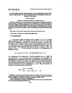
FIG. 2. The coefficient of the L2 solution in Eqs (109-116) with the largest peak. In this particular plot we chose µL = 2, µS = 9/4, µSL = 3, ηL = 0 and also ω = 1. We see that the coefficients are bounded at this ω even as Re(s0 ) → 0. The estimate (118) shows that this holds at every ω.
for all Re(s0 ) > 0 and ω 0 ∈ R with |s0 |2 +|ω 0 |2 = 1. Therefore, the solution of the gauge and metric components at the boundaries are bounded by the given boundary data. Fig. 2 displays the largest coefficient of the above L2 solution for ω 0 → 1 (|s0 | → 0). We note that the solution remains continuously bounded. Thus, there is a positive constant C such that, |˜ α(s, 0, ω)| ≤ C |˜ gα | .
This inequality is the basic estimate in the LaplaceFourier space, but because our boundary conditions contain many derivatives of the primitive fields, a little more book-keeping is required to build an estimate that can be inverted to give an estimate in an appropriate norm, involving higher derivatives of the primitive variables in the physical space. Note, crucially, that the form of the given data, in particular the choice of derivatives, in the boundary conditions is needed to obtain boundary stability. This form cancels terms that would otherwise result in singular behavior breaking boundary stability. This is what prevents us from choosing for example lower order L = 1 conditions. The final estimate: Following [11], where the estimate (58) has been generalized in order to estimate the L2 -norm of the higher derivatives of the primitive fields in terms of the L2 -norm of the given boundary data for all Re(s) > 0 and all smooth solutions u with the property that its L + 1-time derivatives vanish identically at t = 0, we multiply the inequality (123) by κ8 to obtain an estimate for the tangential derivatives to the boundary. For the normal derivatives, namely second or higher derivatives of the fields, we use the equations of motion (74) to obtain, Z∞ X 5 � 3 5−l l 2 X 5−l l ˜ 2 κ ∂x α ˜ + η κ ∂x βi 2 � + κ5−l ∂xl γ˜ij dx 3 � 2 X 5−l l ˜ 2 + κ5−l ∂xl α ˜ + κ ∂x βi
(119)
Similar arguments hold for the other components. We conclude that the full solution of the system with fifth order BCs satisfies the estimate 0
|˜ u(s, x = 0, ω)| ≤ C |˜ g (s, ω)| ,
i=1
2 � + κ5−l ∂xl γ˜ij
(120)
for all Re(s) > 0 and ω ∈ R with C 0 > 0 a positive constant. We then conclude that the above system is boundary stable [70]. As we have seen in section III C, ˆ = R(s ˆ 0 , ω 0 ) such it implies that there is a symmetrizer R that [11], D E D E ˆu ˆ ∂x u ∂x u ˜, R ˜ =2 u ˜, R ˜ � E D � ˆ M + M∗ R ˆ u = u ˜, R ˜ . (121) Here we have used the equations of motion. Using the ˆ we obtain first and second properties of R, D E ˆu ∂x u ˜, R ˜ ≥ C1 η |˜ u|2 , (122) with η = Re(s). Integrating both sides from x = 0 to x = ˆ it ∞ and using the last property of the symmetrizer R, follows that Z ∞ 1 D ˆ E η |˜ u|2 dx ≤ − u ˜, R u ˜ C1 x=0 0 � 1 ≤ −C3 |˜ u|2 x=0 + C2 |˜ g |2 . (123) C1
i=1
l=0
0
≤C
�
x=0
� ˜ α | + · · · + |κ Im(h ˜ Ψ )|2 , |κ h 0 5
2
5
(124)
for some strictly positive constant C > 0. Finally, integrating over Im(s) and over all frequencies ωA and using Parseval’s relation we obtain [11], X X η kαk2η,5,Ω + η kβ i k2η,5,Ω + η kγij k2η,5,Ω + i
η kαk2η,5,T
+η
ij
X
kβ i k2η,5,T
i
≤ C5
khα k2η,5,T
+η
X
kγij k2η,5,T
ij
+ ··· +
khΨ0 k2η,5,T
�
,
(125)
where C5 is a positive constant, Ω is, as we have mentioned before, the domain of integration, T is the boundary surface and the above L2 -norms are defined by, kuk2η,5,Ω = Z X ρ e−2 η t |∂t t ∂xρx ∂yρy ∂zρz u(t, x, y, z)|2 dΩ , (126) Ω
|ρ|≤5
kuk2η,5,T Z T
=
e−2 η t
X |ρ|≤5
|∂tρt ∂xρx ∂yρy ∂zρz u(t, 0, y, z)|2 dT . (127)
18 Here ρ = (ρt , ρx , ρy , ρz ) is a multi-index, and we denote dΩ = dt dx dy dz and dT = dt dy dz. Adding forcing terms to the equations of motion modifies the estimate (125) in the standard way. Here we have dropped the forcing terms F from the estimates, but these can also be dealt with exactly as in [11]. The above result can be easily generalized for high order conditions. One can show that, once we have a regular L2 -solution for given BCs, i. e. regular coefficients for all ω 0 ∈ R and Re(s0 ) > 0, increasing the order the derivatives at the boundary does not generate singular coefficients. One then can show that the resulting IBVP is boundary stable and use the above procedure to show that the problem is well-posed.
H.
Why work under the boundary orthogonality condition?
We saw in the previous sections that using the boundary orthogonality condition results in the simplification ˚ = 0 in the Laplace-Fourier analysis. Since we are that β able to construct the general L2 solution even without this restriction it is natural to ask why we do so. The reason is that to pick natural boundary conditions it is very helpful if the symbol M has a simple eigendecomposition, for then we may look at the left eigenvectors of M contracted with the state vector u ˜ and essentially read off sensible boundary conditions. Therefore the defi˚ω 0 is a very serious ciency of M in the special case s0 = −β problem, because conditions that work elsewhere in frequency space fail to give control at these special points. The special case appears because at this particular frequency all of the relevant eigenvalues, the different τµ− , many of which are generically distinct, clash. When this happens the associated eigenspace has to support many more eigenvectors, but can not. Under the boundary ˚ = 0 this breakdown of orthogonality condition with β diagonalizability occurs at s0 = 0, but is not a problem because for boundary stability we are concerned with the solution in the limit s0 → 0. It may be possible to find boundary conditions that are well-behaved also across ˚ω 0 , but doing so will result in the bad frequency s0 = −β several other deficiencies. Such conditions will necessarily require more complicated mixing of the eigensolutions in the analysis. This will result in more complicated absorption properties and in difficult estimates to perform, for which we do not presently have adequate computer algebra tools. Therefore it is highly desirable to side-step the special case completely. Several strategies for this are apparent. The first of these is to try and choose a formulation for which the special case does not appear. Even if we fix the gauge choice, one might hope that this is possible by adjusting the constraint subsystem, and how it is coupled to the gauge variables. We have attempted this [67] within the large class of formulations considered in [48], but to no avail. The missing eigenvectors are associated
˜ variable but since this is not a constraint, with the Λ such adjustments do not help. Thus the next option is to change the gauge conditions, which we do under duress, because we would like to show well-posedness for arbitrary hyperbolic gauges. The highly restricted class containing the harmonic gauge (76) suffices. From the PDEs point of view is perhaps not surprising; the simple characteristic structure of the restriction eradicates nearly all coupling between different metric components, but this it must do so that hyperbolicity can be achieved with many shared speeds. The symbol M inherits, to a large extent, the same decoupling. It may be that these gauges then allow for estimates with fewer derivatives, and without using the boundary orthogonality condition. Certainly this is the case for the harmonic gauge. Throughout we have focused on evolved gauge conditions where the time derivative is naturally given in the form α−1 (∂t − β i ∂i ). The next option for adjusting the gauge, which we have not investigated but which we do think may help avoid the special case, is to switch to conditions built naturally on the time derivative ∂t . In applications one can easily transition from the first form to the second, and we expect that in this way the special case can be cured, at least for some gauge conditions. As mentioned earlier on, we also expect that once a well-posed IBVP is obtained with a particular formulation it will be straightforward to obtain well-posedness by employing the dual-foliation formalism [50]. We furthermore expect that in this way one will naturally obtain geometric uniqueness. The final obvious strategy is to work under the boundary orthogonality condition so that the special case simply does not occur. This solution is inconvenient the point of view of numerical implementation both because of the drifting boundary, and, depending on the gauge choice, because of the number of derivatives present in the boundary conditions. But this approach is geometrically natural, allowed us to demonstrate boundary stability for a wide range of gauge conditions and as shown in section II D allows reasonable approximations of the desired conditions to be implemented straightforwardly.
IV.
CONCLUSION
To obtain solutions of the Cauchy problem for asymptotically flat spacetimes in numerical GR, one option is to make the computational domain as large as possible so that the boundary remains causally disconnected from the central body. Unfortunately the computational cost of this option is prohibitive, even if one uses meshrefinement or compactification to spatial infinity, because numerical error can travel faster than physical effects. A second, much more elegant, possibility is to evolve initial data which is hyperboloidal, that is, compactified to null infinity [73–80], or, along similar lines of thought data in which a Cauchy region is attached to a null outer zone [81, 82]. Many obstacles are still to be overcome before such data can be routinely evolved, which means that
19 in the immediate future we are left with one option; the specification of improved outer boundary conditions for applications. As greater accuracy is required of numerical data, or when the boundary becomes an integral part of the physics of the system, as in the case of asymptotically AdS spacetimes [83–85], boundary conditions must be carefully considered. In this paper, we were concerned with boundary conditions appropriate for the evolution of asymptotically flat spacetimes with the moving puncture method. We considered constraint preserving conditions for free-evolution formulations of the Einstein equations coupled to a parametrized set of dynamical gauge choices. We derived a new class of high order boundary conditions for this family of gauge conditions. To reduce the amount of spurious gravitational wave reflections, we also employ a high order freezing-Ψ0 condition [4, 61]. We analyzed wellposedness of the resulting initial boundary value problem on a four dimensional spacetime with timelike outer boundary by considering high-frequency perturbations of a given smooth background solution. Using the LaplaceFourier transform we showed that the resulting IBVP is boundary stable. The Kreiss-Agranovich-M´etivier theory, valid even when the system is only strongly hyperbolic of constant multiplicity, guarantees that the IBVP is well-posed in the frozen coefficient approximation. By virtue of the theory of pseudo-differential operators, the general problem is expected to be well-posed too. These results generalize our previous study [5] in which the constraint absorption properties of the CPBCs were considered. This work could be generalized in a number of ways. Firstly one could consider a larger family of dynamical
gauge conditions. We do not expect such a generalization to be very taxing, provided that one is still able to make the necessary manipulation of the symbol M by computer algebra. Another possibility is to maintain the same family of gauge conditions but to alter the boundary conditions. By construction our boundary conditions are those that render the proof of boundary stability as close as possible to that of the wave equation. Therefore, besides the trivial reflecting case, we expect that other choices will rapidly become intractable. One might also consider in what approximation, if any, a finite difference approximation to the IBVP could be shown to be formally numerically stable. Finally one could examine how readily the present calculations could be extended to other formulations of GR.
[1] H.-O. Kreiss, Numerical Methods for Solving TimeDependent Problems for Partial Differential Equations (Les Presses De L’Universit´e de Montr´eal (University of Montreal Press), Montreal (Canada), 1978), ISBN ISBN 0-8405-0430-6. [2] H. O. Kreiss and J. Lorenz, Initial-boundary value problems and the Navier-Stokes equations (Academic Press, New York, 1989). [3] M. Miller, P. Gressman, and W.-M. Suen, Phys. Rev. D 69, 064026 (2004), gr-qc/0312030. [4] L. T. Buchman and O. C. A. Sarbach, Class. Quant. Grav. 23, 6709 (2006), gr-qc/0608051. [5] M. Ruiz, D. Hilditch, and S. Bernuzzi, Phys. Rev. D 83, 024025 (2011), 1010.0523. [6] D. Givoli, Journal of Computational Physics 94, 1 (1991). [7] H. Friedrich and G. Nagy, Commun. Math. Phys. 201, 619 (1999). [8] H.-O. Kreiss and J. Winicour, Class. Quantum Grav. 23, S405 (2006), gr-qc/0602051. [9] O. Rinne, Class. Quant. Grav. 23, 6275 (2006), grqc/0606053.
[10] H. Kreiss, O. Reula, O. Sarbach, and J. Winicour, Class.Quant.Grav. 24, 5973 (2007). [11] M. Ruiz, O. Rinne, and O. Sarbach, Class. Quant. Grav. 24, 6349 (2007), 0707.2797. [12] H.-O. Kreiss, O. Reula, O. Sarbach, and J. Winicour, Commun.Math.Phys. 289, 1099 (2009), 0807.3207. [13] H. Friedrich, Comm. Math. Phys. 100, 525 (1985). [14] H. Friedrich, Comm. Math. Phys. 107, 587 (1986). [15] D. Garfinkle, Phys. Rev. D 65, 044029 (2002), grqc/0110013. [16] F. Pretorius, Class. Quant. Grav. 22, 425 (2005), grqc/0407110. [17] F. Pretorius, Phys. Rev. Lett. 95, 121101 (2005), grqc/0507014. [18] L. Lindblom, M. A. Scheel, L. E. Kidder, R. Owen, and O. Rinne, Class. Quant. Grav. 23, S447 (2006), grqc/0512093. [19] M. Boyle, L. Lindblom, H. Pfeiffer, M. Scheel, and L. E. Kidder, Phys. Rev. D75, 024006 (2007), gr-qc/0609047. [20] H. P. Pfeiffer, D. A. Brown, L. E. Kidder, L. Lindblom, G. Lovelace, and M. Scheel, Classical Quantum Gravity 24, S59 (2007), gr-qc/0702106.
ACKNOWLEDGMENTS
It is a pleasure to thank Bernd Br¨ ugmann, Luisa Buchman, Ronny Richter and especially Olivier Sarbach for helpful discussions and comments on the manuscript. This work was supported in part by DFG grant SFB/Transregio 7 “Gravitational Wave Astronomy”, by Spanish Ministry of Science and Innovation under grants CSD2007-00042, CSD2009-00064 and FPA2010-16495, the Conselleria d’Economia Hisenda i Innovaci´o of the Govern de les Illes Balears and by Colciencias under program “Es tiempo de Volver”. We also wish to acknowledge to the ESI and to the organizers of the ESI workshop on “Dynamics of General Relativity: Numerical and Analytical Approaches”, July - September, 2011, where part of this work was developed.
20 [21] J. Seiler, B. Szilagyi, D. Pollney, and L. Rezzolla, Class. Quant. Grav. 25, 175020 (2008), 0802.3341. [22] D. Hilditch, A. Weyhausen, and B. Brgmann, Phys. Rev. D93, 063006 (2016), 1504.04732. [23] T. W. Baumgarte and S. L. Shapiro, Phys. Rev. D 59, 024007 (1998), gr-qc/9810065. [24] M. Shibata and T. Nakamura, Phys. Rev. D 52, 5428 (1995). [25] T. Nakamura, K. Oohara, and Y. Kojima, Prog. Theor. Phys. Suppl. 90, 1 (1987). ˇ aˇcek, [26] C. Bona, T. Ledvinka, C. Palenzuela, and M. Z´ Phys. Rev. D 67, 104005 (2003), gr-qc/0302083. ˇ aˇcek [27] C. Bona, T. Ledvinka, C. Palenzuela, and M. Z´ (2003), gr-qc/0307067. [28] S. Bernuzzi and D. Hilditch, Phys. Rev. D 81, 084003 (2010), 0912.2920. [29] A. Weyhausen, S. Bernuzzi, and D. Hilditch, Phys. Rev. D 85, 024038 (2012), 1107.5539. [30] D. Alic, C. Bona-Casas, C. Bona, L. Rezzolla, and C. Palenzuela, Phys. Rev. D 85, 064040 (2012), 1106.2254. [31] Z. Cao and D. Hilditch, Phys. Rev. D 85, 124032 (2012), 1111.2177. [32] D. Alic, W. Kastaun, and L. Rezzolla, Phys. Rev. D88, 064049 (2013), 1307.7391. [33] C. Bona, J. Mass´ o, E. Seidel, and J. Stela, Phys. Rev. Lett. 75, 600 (1995), gr-qc/9412071. [34] M. Alcubierre, Class. Quantum Grav. 20, 607 (2003), gr-qc/0210050. [35] J. G. Baker, J. Centrella, D.-I. Choi, M. Koppitz, and J. van Meter, Phys. Rev. Lett. 96, 111102 (2006), grqc/0511103. [36] M. Campanelli, C. O. Lousto, P. Marronetti, and Y. Zlochower, Phys. Rev. Lett. 96, 111101 (2006), grqc/0511048. [37] J. R. van Meter, J. G. Baker, M. Koppitz, and D.-I. Choi, Phys. Rev. D 73, 124011 (2006), gr-qc/0605030. [38] C. Gundlach and J. M. Martin-Garcia, Phys. Rev. D 74, 024016 (2006), gr-qc/0604035. [39] M. Alcubierre, Introduction to 3+1 Numerical Relativity (Oxford University Press, Oxford, 2008). [40] H. Beyer and O. Sarbach, Phys. Rev. D 70, 104004 (2004), gr-qc/0406003. [41] D. Nunez and O. Sarbach, Phys. Rev. D81, 044011 (2010), 0910.5763. [42] M. Ruiz, J. C. Degollado, M. Alcubierre, D. Nunez, and M. Salgado, Phys. Rev. D86, 104044 (2012), 1207.6142. [43] M. Alcubierre and J. M. Torres, Class. Quant. Grav. 32, 035006 (2015), 1407.8529. [44] O. Sarbach and M. Tiglio, Living Reviews in Relativity 15 (2012), 1203.6443, URL http://www.livingreviews. org/lrr-2012-9. [45] C. Bona, T. Ledvinka, C. Palenzuela-Luque, and M. Zacek, Class. Quantum Grav. 22, 2615 (2005), grqc/0411110. [46] C. Bona and C. Bona-Casas, Phys. Rev. D82, 064008 (2010), 1003.3328. [47] D. Hilditch, S. Bernuzzi, M. Thierfelder, Z. Cao, W. Tichy, and B. Br¨ ugmann, Phys. Rev. D 88, 084057 (2013), 1212.2901. [48] D. Hilditch and R. Richter, Phys. Rev. D94, 044028 (2016), 1303.4783. [49] G. I. Eskin, Boundary value problems for elliptic pseudodifferential equations; Translations of mathematical mono-
[50] [51]
[52] [53]
[54] [55] [56] [57] [58] [59] [60] [61] [62] [63] [64] [65] [66]
[67] [68] [69] [70] [71] [72] [73] [74] [75] [76] [77] [78] [79] [80]
graphs, V. 52 (American Mathematical Society, Providence, R.I., 1981). D. Hilditch (2015), 1509.02071. C. Gundlach, J. M. Martin-Garcia, G. Calabrese, and I. Hinder, Class. Quantum Grav. 22, 3767 (2005), grqc/0504114. C. Bona, J. Mass´ o, E. Seidel, and J. Stela, Phys. Rev. Lett. 75, 600 (1995), gr-qc/9412071. M. Alcubierre, B. Br¨ ugmann, P. Diener, M. Koppitz, D. Pollney, E. Seidel, and R. Takahashi, Phys. Rev. D 67, 084023 (2003), gr-qc/0206072. E. Schnetter, Class. Quant. Grav. 27, 167001 (2010), 1003.0859. D. M¨ uller and B. Br¨ ugmann, Class. Quant. Grav. 27, 114008 (2010), 0912.3125. D. Alic, L. Rezzolla, I. Hinder, and P. Mosta, Class. Quant. Grav. 27, 245023 (2010), 1008.2212. O. Rinne, Ph.D. thesis, University of Cambridge, Cambridge, England (2005), gr-qc/0601064. D. Hilditch (2017). O. Sarbach and M. Tiglio, Journal of Hyperbolic Differential Equations 2, 839 (2005), gr-qc/0412115. O. Rinne, L. Lindblom, and M. A. Scheel, Class. Quant. Grav. 24, 4053 (2007), 0704.0782. L. T. Buchman and O. C. Sarbach, Class.Quant.Grav. 24, S307 (2007), gr-qc/0703129. H. Witek, D. Hilditch, and U. Sperhake, Phys. Rev. D83, 104041 (2011), 1011.4407. D. Pollney, C. Reisswig, E. Schnetter, N. Dorband, and P. Diener, Phys. Rev. D 83, 044045 (2011), 0910.3803. A. Bayliss and E. Turkel, Communications in Pure Applied Mathematics 33, 707 (1980). O. Rinne, L. T. Buchman, M. A. Scheel, and H. P. Pfeiffer, Class. Quant. Grav. 26, 075009 (2009), 0811.3593. B. Gustafsson, H.-O. Kreiss, and J. Oliger, Time dependent problems and difference methods (Wiley, New York, 1995). https://www.tpi.uni-jena.de/tiki-view_tracker_ item.php?itemId=254. G. Nagy, O. E. Ortiz, and O. A. Reula, Phys. Rev. D 70, 044012 (2004). C. Gundlach and J. M. Mart´ın-Garc´ıa, Class. Quantum Grav. 23, S387 (2006), gr-qc/0506037. H.-O. Kreiss, Comm. Pure Appl. Math. 23, 277 (1970). M. S. Agranovich, Functional Analysis and Its Applications 6, 85 (1972), ISSN 0016-2663. G. M´etivier, Bulletin of the London Mathematical Society 32, 689 (2000). J. Frauendiener, Living Rev. Relativity 7 (2004), http://www.livingreviews.org/lrr-2004-1. G. Calabrese, C. Gundlach, and D. Hilditch, Class.Quant.Grav. 23, 4829 (2006), gr-qc/0512149. A. Zengino˘ glu and S. Husa, Class. Quantum Grav. 25, 19 (2008), gr-qc/0612161. A. Zenginoglu, Class. Quant. Grav. 25, 195025 (2008), 0808.0810. V. Moncrief and O. Rinne, Class.Quant.Grav. 26, 125010 (2009), 0811.4109. L. T. Buchman, H. P. Pfeiffer, and J. M. Bardeen, Phys.Rev. D80, 084024 (2009), 0907.3163. O. Rinne, Class.Quant.Grav. 27, 035014 (2010), 0910.0139. A. Va˜ no ´ Vi˜ nuales, S. Husa, and D. Hilditch, Class. Quant. Grav. 32, 175010 (2015), 1412.3827.
21 [81] J. Winicour, Living Rev. Relativity 1, 5 (1998), [Online article], URL http://www.livingreviews.org/ lrr-1998-5. [82] C. Reisswig, N. T. Bishop, D. Pollney, and B. Szilagyi, Phys. Rev. Lett. 103, 221101 (2009), 0907.2637.
[83] P. Bizon and A. Rostworowski, Phys. Rev. Lett. 107, 031102 (2011), 1104.3702. [84] H. Bantilan, F. Pretorius, and S. S. Gubser, Phys. Rev. D85, 084038 (2012), 1201.2132. [85] V. Cardoso, L. Gualtieri, C. Herdeiro, U. Sperhake, P. M. Chesler, et al. (2012), 1201.5118.