ability to provide more than local, one-dimensional support. Between the
strategic ... teleoperation of a Kawasaki Mule through a similar field. (Section V).
The Intelligent CoPilot A Constraint-Based Approach to Shared-Adaptive Control of Ground Vehicles Sterling J Anderson, James M. Walker, Sisir B. Karumanchi, and Karl Iagnemma Dept. of Mechanical Engineering Massachusetts Institute of Technology Cambridge, MA, USA {ster | sisir | kdi} @mit.edu Abstract—This paper presents a new approach to semiautonomous vehicle hazard avoidance and stability control, based on the design and selective enforcement of constraints. This differs from traditional approaches that rely on the planning and tracking of paths and facilitates “minimallyinvasive” control for human-machine systems. Instead of forcing a human operator to follow an automation-determined path, the constraint-based approach identifies safe homotopies, and allows the operator to navigate freely within them, introducing control action only as necessary to ensure that the vehicle does not violate safety constraints. This method evaluates candidate homotopies based on “restrictiveness”, rather than traditional measures of path goodness, and designs and enforces requisite constraints on the human’s control commands to ensure that the vehicle never leaves the controllable subset of a desired homotopy. This paper demonstrates the approach in simulation and characterizes its effect on human teleoperation of unmanned ground vehicles via a 20-user, 600-trial study on an outdoor obstacle course. Aggregated across all drivers and experiments, the constraintbased control system required an average of 43% of the available control authority to reduce collision frequency by 78% relative to traditional teleoperation, increase average speed by 26%, and moderate operator steering commands by 34%. Keywords—Semi-Autonomous control, shared adaptive control, planning, obstacle avoidance, unmanned ground vehicles, teleoperation, human-machine interaction
I.
INTRODUCTION
Humans make mistakes. When humans control dynamic systems, the rate and ramifications of those mistakes increase. Whether it occurs while driving a car, controlling industrial machinery, or teleoperating an unmanned vehicle, human error can lead to costly and often deadly consequences. In 2010, over 32,000 people were killed and another 2.2 million injured in motor vehicle accidents in the United States alone [1]. The U.S. military is also strongly affected by human error, with vehicle crashes representing the leading cause of non-hostile deaths in Operation Iraqi Freedom [2]. Even unmanned ground vehicles are susceptible, as operators must not only cope with the challenges inherent to the manned driving task, but must perform many of the same functions with a restricted field of view, limited depth perception, potentially disorienting camera viewpoints, and significant time delays [3]. Remotely operating a ground vehicle under these conditions while monitoring the vehicle’s health status, the status of the
Quantum Signal, LLC Saline, MI, USA
[email protected]
mission/tasks, and the condition of the environment leads to high failure rates, with many of today’s UGV’s failing before having completed even one full shift [4]. Semi-autonomous control offers a unique opportunity to improve human performance through the exploitation of human-automation synergies. As originally published in 1951 [5] and widely discussed since, humans and automation are uniquely well suited to specific types of tasks [6]. Whereas automation excels at responding quickly and precisely to well-defined or repetitive control objectives, humans tend to make more mistakes as the frequency and complexity of the control task increase. Conversely, humans have the unique ability to detect and contextualize patterns and new information, reason inductively, and adapt to new modes of operation, whereas automation typically struggles at these tasks. The goal of semi-autonomy is to exploit synergies in the abilities of humans and automation to improve planning and control performance of the combined system and – where possible – the actors therein. A. Previous Work Research to date in vehicle control has left a significant gap between fully-autonomous planning and control frameworks, which neither account for nor provide an effective means of cooperating with the human operator, and driver assistance systems which are typically limited to local, one-dimensional support. While these classes of system are distinct in their intended outcomes, their inability to effectively share control with a human driver has its root in a common, basic building block: each relies on specific, planned paths. In the context of autonomous control, many methods exist for planning paths. Common path planning tools include rapidly-exploring random trees [7], graph search methods [8], potential fields [9], and neural optimization techniques [10]. Control laws routinely used to track these reference paths include PID schemes, linear-quadratic regulators, and nonlinear fuzzy controllers. While many variations of this planning-then-control approach have proven effective in autonomous implementations [11], their reliance on a specific reference path (which is in many cases arbitrary, non-intuitive, and over-restrictive to a human operator), and consequent inability to account for the planning preferences and control inputs of a human operator make them ill-suited for human-in-the-loop or “semiautonomous” control.
At the other end of the vehicle safety community, with an eye on nearer-term, industry-driven objectives, researchers have developed systems that assist the human operator in avoiding collisions and loss of stability. These “active safety systems” traditionally fall into one of two categories: reactive safety systems, such as antilock brakes, traction controllers, electronic stability controllers, and lane-assist approaches monitor the current state of the vehicle and apply low-level control actions to meet some safety-critical criteria [12]. Predictive safety systems, on the other hand, consider not only the current state of the ego vehicle, but also the predicted state evolution of the vehicle and environmental hazards. These systems then preemptively assist the driver in identifying, assessing the threat posed by, and in some cases avoiding an impending hazard. Recent work in predictive safety has resulted in systems that use audible warnings [13], haptic alerts [14] and steering torque overlays [15] to help the driver avoid collisions [16], instability [17], or lane departure [18]. Similar to autonomous systems, the pathbased prediction metrics used by these systems limits their ability to provide more than local, one-dimensional support. Between the strategic, multidimensional capabilities of autonomous planning and control systems and the more tactical, one-dimensional focus of driver-assistance systems lies a significant need for truly semi-autonomous navigation; planning and control techniques capable of both strategic planning and intuitive, “intention-preserving” control support. We posit that such a system should be designed to accommodate the field-based planning and control technique humans have long been shown to exhibit [19]. Rather than obsessively planning and tracking a single path, humans tend instead to identify a field of safe travel – one that contains an infinite number of continuously deformable (“homotopic”) paths – and control the vehicle within it. This homotopy selection arguably represents the highest level of human reasoning employed in the navigation task and reduces the subsequent burden of calculating and applying appropriate control inputs to that of simply remaining within the desired homotopy. On an open roadway, for example, the preferred homotopy often contains many acceptable paths traversing a desired lane. In off-road environments, the desired homotopy may not be as clearly delineated, though vehicle dynamic constraints require that it exclude any region through which the vehicle cannot travel without colliding with obstacle(s). Figure 1 illustrates three prominent homotopies in a cluttered environment as they might be perceived by a human operator.
Figure 1. Visualization of prominent homotopies available to a human operator (image best viewed in color).
Instead of planning a path and restricting the human operator to that path, we propose a constraint-based semiautonomous system that strategically limits the range of available inputs to ensure that the operator retains as much control freedom as possible without risking collision with obstacles or dynamic instability. B. Paper Outline This paper introduces a new approach to semiautonomous control; one in which homotopies and their associated constraints are identified, characterized, planned, and enforced to ensure that the controlled system (an offroad ground vehicle in this case) avoids hazards and loss of stability without unduly restricting the control freedom of a human operator. Section II describes the methods used to plan and characterize constraints on the vehicle position. Section III then describes one method for converting those constraints into semi-autonomously enforceable constraints on the operator’s control commands. These methods are demonstrated in control of a simulated ground vehicle through an obstacle field (Section IV) and semi-autonomous teleoperation of a Kawasaki Mule through a similar field (Section V). The paper then closes with general conclusions. II.
CONSTRAINT PLANNING
Planning in constraint or “homotopy space” requires the identification of homotopies and an evaluation of their goodness. However, because the constraints bounding a homotopy admit an infinite number of paths, identifying and evaluating the “goodness” of these constraints requires a new set of evaluation criterion from those commonly used in path planning. Whereas the goodness or “optimality” of a specific path is well defined using metrics such as length, curvature, and dynamic feasibility, corresponding measures lose their traditional meaning when applied to a set of constraints and the many paths they admit. Further, planning methods typically used to design paths, such as graph search, potential fields, and sampling-based algorithms, will not necessarily work to plan constraints since the latter must be designed to circumscribe – rather than simply remain within – a safe operating region. In light of this inherent difficulty, a method is presented here based on the constrained Delaunay triangulation, which provides a useful physical boundary to, and heuristic evaluation of, the many distinct paths existing within a given homotopy. A. Homotopy Identification As illustrated in Figure 1, any environment bifurcated by obstacles or impassible regions admits multiple path homotopies. A path homotopy is a set of paths that can be continuously deformed into one another without crossing infeasible regions. If a particular homotopy can be identified, vehicle position constraints may be designed at its edges to circumscribe the set of paths it contains and thereby ensure that the vehicle remains safely within it (avoiding collisions with obstacles). In this work, we identify homotopies by decomposing a two-dimensional configuration space into a complete set of constrained Delaunay triangles. The dual graph of this triangulation provides a search space through which homotopies may be planned via standard graph search
methods. That is, any feasible homotopy containing the vehicle’s current position X0, and the position of the goal location, XG, may be defined as a sequence Hn of adjacent triangles T0…Tn extending from the triangle circumscribing the vehicle’s current position (T0 in Figure 2) to that containing the goal location(s). This goal may be described by a single point or by a given region of R2, such as the distal edge of the local sensing window illustrated in red in Figure 2. B. Homotopy Evaluation In order to plan a set of constraints circumscribing a desired homotopy, metrics describing homotopy goodness must be defined and ascribed to individual triangles and transitions between them. We here propose geometric and reachability heuristics for evaluating homotopy goodness. These include an estimate of the average “distance” traveled by paths within it, an estimate of the control freedom it affords an operator, and an approximation of its dynamic reachability given the vehicle’s current state and control input. Given a constrained Delaunay triangulation of C, we note that any path belonging to a particular homotopy will pass through each triangle Tk in Hn at least once. A path enters Tk through the edge it shares with Tk-1 (Ek-1, k) and exits through Ek, k+1 into Tk+1. Thus, the average “distance” traveled by all triangle-monotonic (passing through each edge at most once) paths belonging to a given homotopy as it crosses Tk may be heuristically described as the distance from the midpoint of Ek-1,k to that of Ek,k+1. As Figure 2 illustrates, the dual graph embodying this heuristic closely resembles the Generalized Voronoi Diagram (GVD).
may be characterized by the lateral acceleration it requires. 2.
This lateral acceleration is directly proportional to the square of vehicle velocity and inversely proportional to the radius of curvature of the path it follows.
3.
In any homotopy Hn, the maximum radius of curvature of any of the constant-velocity paths belonging to Hn is limited by the “width” wk, or minimum pass-through clearance of the Delaunay Triangles comprising the homotopy. As illustrated in Figure 3, wk is calculated as the perpendicular distance from the constrained edge of the triangle to the apex opposite the constrained edge. If Tk is obtuse and either Ek-1,k or Ek,k+1 lie opposite the obtuse vertex, wk is instead calculated as the shorter of Ek-1,k and Ek,k+1.The blue dashed line in Figure 3 illustrates the maximal radius path belonging to a particular homotopy.
4.
This maximal curvature is also affected by the relative orientation of adjacent constrained edges, or equivalently, the difference in orientation ϕk-1,k for adjacent line segments Lk-1 and Lk of the dual graph used to calculate “length” (these being parallel to the constrained edge).
Figure 3. Illustration of a triangulated channel and the heuristics used to describe constraint restrictiveness and dynamic feasibility
Figure 2. Illustration of triangulated environment showing homotopy selection and dual graph for length heuristic
While the average “length” of paths belonging to a particular homotopy may be described by the distance metric above, the “restrictiveness” and dynamic feasibility of the constraints bounding this homotopy require heuristic evaluations of the range of motion and control freedom they admit. To incorporate these considerations into the constraint-planning problem, we observe the following: 1.
The dynamic feasibility of any path followed by a vehicle with Dubins constraints and friction-limited tires
Finally, while the above heuristics give an estimate of the dynamic feasibility of a set of constraints, they do not explicitly account for the dynamic reachability of the homotopy itself from the vehicle’s current state. This consideration is incorporated into the homotopy planning layer using an adaptation of the dynamic window approach originally described in [20]. Rather than map obstacles onto a 2-dimensional velocity search space, however, our approach instead maps the total vehicle acceleration required to avoid obstacles onto the one-dimensional steering space of the vehicle. It then calculates the surplus tire friction available to the human driver if s/he were to steer into either homotopy. Steering angles from which the vehicle cannot avoid a collision with an impending obstacle are excluded from this area calculation. Figure 4b illustrates one such region (labeled “Collision Imminent”) corresponding to a range of steering angles from within which the vehicle cannot avoid the black obstacle at its current speed.
Summed over the steering angles corresponding to the homotopy choices, the surplus tire friction for homotopy i is then given by
(4)
where δE1, ● (1) and δE1, ● (2) are the extremal steering angles reaching the two ends of edge E1,● (edges of the “Collision Steer” regions illustrated in Figure 4), δ●actuator refers to physical steering limits, and δ●kinematic represents the maximum non-slip steering angle allowed by the tire friction
(a)
and current vehicle velocity
.
With heuristics Lk, wk, ϕk, and a*surplus thus calculated, a graph search (Dijkstra’s algorithm is used here) may be performed to calculate the optimal path homotopy (a “channel” made of adjacent triangles) and its associated constraints. In the results shown in this paper, the objective function is defined as (5)
(6)
(b) Figure 4. Illustration showing a) triangularized environment with obstacles (gray and black), and b) avoidance acceleration mapped to steering commands (with gray and black blocks corresponding to obstacles in (a).
Assuming constant velocity V, wheelbase length L, tire friction coefficient μ, gravity g, stationary obstacles, and noslip conditions (turns of constant radius), the minimal avoidance acceleration required to avoid obstacle ● is given by
III.
CONSTRAINT ENFORCEMENT
In the previous section, an objective function was defined to assess the goodness of a given homotopy. Once a desired homotopy has been identified, vehicle position constraints circumscribing the homotopy must be converted into semiautonomously enforceable constraints on the human operator’s control inputs as the vehicle traverses the constrained region.
(2)
To calculate these limits, a finite-horizon model predictive (MPC) controller is used to predict the vehicle state evolution within the desired homotopy under a stabilityoptimal control input sequence. The nearness of the predicted trajectory to stability limits is then used to compute the steering constraint applied at the vehicle and the torque feedback provided to the operator. These steps are briefly described below.
(3)
The MPC controller bases its predictions on a 4-wheeled vehicle model with slip and yaw dynamics. Defining vehicle states, outputs, inputs, and disturbances by x, y, u, and v, respectively, discrete plant dynamics are described by
(1) ,
where
, and .
This objective function incorporates an estimate of average homotopy “length” with an approximation of the control freedom and dynamic stability available to the vehicle as it traverses the homotopy.
Below a configurable threshold Φeng, K=0 and the driver retains full control authority. Above Φaut, K=1, and the MPC controller operates autonomously to satisfy state and y k = Cx k + Dv v k . (8) homotopy constraints. Between Φeng and Φaut, control A quadratic objective function over a prediction horizon authority is shared. of p sampling intervals is defined as This intervention ensures that at low threat, the vehicle k + p −1 k + p −1 k+ p closely matches operator commands while at high threat – 1 T 1 T 1 1 T 2 J k = ∑ y i R y y i + ∑ ui R u ui + ∑ ∆ui R ∆u ∆ui + ρε ε (9) when the safest maneuver satisfying homotopy constraints 2 i=k 2 i=k 2 i = k +12 approaches the limit of vehicle stability – the vehicle steering where Ry, Ru, and R∆u represent diagonal weighting command tracks the optimal command predicted by the , ρε matrices penalizing deviations from MPC controller. For a complete treatment of this threat assessment and shared control method, the reader is referred represents the penalty on constraint violations, n denotes the to the authors’ previous work [21]. number of free control moves, and ε represents the In addition to constraints imposed on (or adjustments maximum constraint violation over the prediction horizon p. made to) the vehicle steering (which is transparent to the Inequality constraints on vehicle position (y), inputs (u), and human operator), experimental tests also fed back a visual input rates (Δu) are then defined as representation of the safe homotopy and a tactile set of “soft” j j j j j constraints on the position of the steering wheel. This y min (i ) − εV min (i ) ≤ y (k + i + 1 | k ) ≤ y max (i ) + εV max (i ) feedback was provided to improve the human operator’s j j j u min (i ) ≤ u (k + i + 1 | k ) ≤ u max (i ) telepresence and situational awareness by indicating not only (10) where the input constraints lie, but also how urgently they ∆u j min (i ) ≤ ∆u j (k + i + 1 | k ) ≤ ∆u j max (i ) must be satisfied in order to avoid collision or loss of control. i = 0,..., p − 1 Visual feedback was provided by overlaying a visual ε ≥0 representation of the desired homotopy on the driver’s screen as illustrated in Figure 5. In addition to the homotopy where the vector ∆u represents the change in input from one overlay, steering angle indicators were provided at the j sampling instant to the next, the superscript “(●) ” bottom of the screen to show the driver where the vehicle is represents the jth component of a vector, k represents the currently steering (red line), and where the driver’s steering current time, and the notation (●)j(k+i|k) denotes the value command lies relative to the vehicle’s current steering angle. predicted for time k+i based on the information available at Section V.A describes the warning indicator. time k. The vector V allows for variable constraint softening over the prediction horizon, p, when ε is included in the objective function. The vectors yymin and yymax are sampled from the edges of the constrained channel Hn. Also note that input constraints enforced in the MPC calculation are simply those imposed by available actuation. The state trajectory predicted by the MPC solution represents the state evolution of maximum stability that can be achieved given the vehicle’s current position, dynamics, and homotopy constraints (imposed by Hn). As such, the nearness of this prediction’s stability-critical states to their physical limits provides a useful indication of the need for intervention and a natural boundary for the current vehicle input. x k +1 = Ax k + B u u k + B v v k
(7)
Here, we define by “threat”, Φ, the maximum predicted value of a stability-critical state (front wheel sideslip in this case). We then adjust the steering command seen by the vehicle (uvehicle) to a blended sum of the optimal (uMPC) and driver (udriver) steering commands
uvehicle = K (Φ )uMPC + (1 − K (Φ ))udriver , where
Figure 5. Illustration of the operator control interface
The resistance torque applied to the operator’s steering wheel is calculated as (13)
(11)
is computed using a piecewise linear
function
(12)
where kmax represents the maximum available steering wheel torque and is used to re-dimensionalize K. Figure 6 illustrates the (hypothetical) response of the torque restoring function to increasingly threatening MPC predictions (assuming the driver fails to steer).
constraints between x=40 and 80 meters allows the human operator to straighten out of desired.
Figure 6. Scenario illustration showing the response of the restoring torque function as a vehicle successively approaches a hazard from behind
Notice that as time progresses (denoted by ti labels on the host vehicle), the threat posed by the optimal maneuver prediction increases. Additionally, the immediate steering command required to track this optimal trajectory begins to drift leftward. The combined effect of an increasinglyurgent, and progressively-leftward uMPC recommendation increases ks and shifts the torque resistance trough. In the limiting case for which only the optimal steering command can reasonably be expected to avoid both the hazard and loss of control (sometime shortly after t4), the controller exerts the maximum available torque on the operator’s steering wheel, essentially ensuring that the operator not only cedes to the requirements of the controller, but is also aware of exactly what steering action is being taken by the vehicle. IV.
SIMULATION TESTING
The constraint-based semi-autonomous controller was simulated using a nonlinear ADAMS model of a generic light truck. The MPC controller ran at 20 Hz. Its prediction and control horizons were calculated over 60 and 40 timesteps, respectively. Parameters in the MPC model were configured to closely match those of the ADAMS plant, vehicle velocity was set at a constant 20 m/s, and simulated driver steering input was set to 0 degrees for generality. Figure 7 shows the path homotopy and associated position constraints designed by the path planner (green channel) as well as the control constraint imposed on the vehicle steering input (colorbar). Note that given the vehicle’s initial position at (0,-2) [m], a shortest-path homotopy would have passed under the obstacles. Because this path is more tortuous and offers less control freedom to the human operator, the objective function described in (5) instead chooses the wider and less dynamically-challenging homotopy passing above the obstacles. Input constraints are initially tight in order to avoid the impending hazard, but quickly relax as the vehicle enters a less restricted region of the homotopy above the obstacles. Finally, we note that the “ricochet” off the upper obstacle occurs because the simulated “human” input remains at zero for the entire maneuver. In practice, the significant control freedom afforded by the relaxed
Figure 7. Simulation results demonstrating constraint-based semiautonomous control through an obstacle field
V.
EXPERIMENTAL TESTING
The effect of constraint-based semi-autonomy and driver feedback on driver performance was tested in a repeated measures study of twenty drivers remotely teleoperating a modified utility vehicle through an obstacle field. Experimental results were analyzed with a one-way analysis of variance (ANOVA) and a significance threshold p = 0.05. A. Setup Experimental testing was performed on a four-wheeled, Kawasaki 4010 Mule utility vehicle fitted with steering and braking actuators, Velodyne LIDAR, NavCom GPS, a triaxial Inertial Measurement Unit (IMU), and a progressive area scan color CCD camera. An onboard Linux PC processed sensing data, ran controller code and transmitted video and other data to a teleoperator control station over an 802.11g wireless link. At the remote control station, human operators received video and state feedback data on a computer monitor and issued steering commands through a Logitech G27 steering wheel. Torque constraints were applied to the steering wheel via its dual-motor force feedback mechanism capable of applying 0-3.1 N-m of torque in either direction. Large barrels were arranged on a 50m x 30m field, and operators were instructed to navigate the course as quickly as possible without hitting them. In order to simulate periodic loss of vision caused by random occurrences such as camera obfuscation, sensor outages, and loss of communication, the camera feed seen by the teleoperator was blanked at random intervals for up to 2 seconds at a time. Twenty operators, ranging in age from 20 to 51 years, with 0-35 years of driving experience, and 0-20+ years of video game experience were tasked with remotely (non-lineof-sight) teleoperating an unmanned ground vehicle across the 50-meter-long by 30-meter-wide obstacle course shown in Figure 8. In addition to this primary task, operators were asked to press a button on the steering wheel every time a warning indicator box in the lower left side of their screen indicated the need. To make this secondary task more challenging, the warning light took three values at random (~2-second) intervals during a trial: “Resting…” (white),
“Don’t Act!” (blue), and “Press Headlights!” (red). Users were instructed to press the button only when this indicator assumed its red, “Press Headlights!” state. Performance on this task was used to gauge differences in cognitive workload required by each control configuration (unassisted vs. assisted).
performance, $150, $100, and $50 gift certificates were promised to the top three finishers. B. Results Figure 9 plots the results of a typical run with shared control and operator feedback enabled. Teleoperation performance was assessed from run data logged at 10 Hz. Dependent measures included collision frequency (collisions/run), course completion time (seconds), driver steer volatility (degrees), reaction time to the secondary task, and overall performance score (seconds).
(a)
(b) Figure 8. Experimental setup (a), constraints (cyan) and MPC prediction (red) on video and LIDAR feed (b)
Prior to the tests, operators were briefed regarding the test setup, control interface, and semi-autonomy details. Each operator manually drove the vehicle through the course before the first round of testing began, and was given one warm-up run with each control configuration prior to each day of testing (first four trials not scored). Altogether, 600 trials were conducted, with 480 of those trials scored (240 scored trials per test configuration). Each operator performed one round of testing per week for three weeks. Testing rounds consisted of 10 total trials (5 trials per configuration), with the configuration order randomized within each round to avoid ordering effects. Barrel placement on the obstacle course was changed between rounds to prevent users from relying on learned habits or worn paths to traverse the course. Following each round of testing, operators were administered an 8-question survey to gauge their acceptance of, comfort with, and confidence in each system configuration. Questions were posed on a 5point Likert scale and included, “How easy was it to navigate the course without collisions,” “How much control did you feel you had over the vehicle’s behavior,” “How fast did you feel comfortable traveling,” and “How confident were you that the vehicle would do the right thing?” Operators were instructed to minimize the performance “score”, where Score = Time + 10*Collisions + 5*Brushes – Hits + Misses. This score represents the total time it takes to navigate the course (in seconds), plus 10-second penalties for each collision, plus 5-second penalties for each “brush” (barrel touched, but does not fall down), and 2-second penalties or rewards for incorrect/correct button presses in response to the secondary task. As an incentive for good
Figure 9. Plot of a typical run showing levels of intervention and its effect on the vehicle steering angle and the feedback provided to the operator
Assessed over all drivers, courses, and dependent measures, constraint-based semi-autonomy improved teleoperational performance. With shared autonomy enabled, the number of collisions decreased by 78% (F(1,478) = 37, p < 1e-8) while average velocity increased by 26% (F(1,478) = 86, p < 1e-18), leading to a corresponding decrease in course completion time (F(1,478) = 91, p < 1e-19) and a 29% improvement in average driver score (F(1,478) = 97, p < 1e20). Figure 10 plots the results of constraint-based semiautonomy on six dependent measures of system performance. With enough control intervention, similar improvements in collision avoidance and average speed might be expected of any controller. What makes this constraint-based framework unique is the minimal degree of adjustments it made to achieve the above results. Averaged across all drivers with shared control and feedback both enabled, the controller took only 43% of the available control authority (mean(K) = 0.43, SD = 0.13) to effect the above performance improvements. This minimal restriction on human
commands afforded the operators significant freedom to maneuver as desired, leading 95% of operators to report feeling a greater sense of both confidence and control with assistance enabled than they felt when left to their own devices. This improvement in performance and confidence was accompanied by a significant decrease in driver steer volatility. With the semi-autonomous controller enabled, drivers were significantly more moderate in their control inputs – decreasing average steering volatility by 34% – from 14.5° to 9.5° (F(1,478) = 147, p < 1e-27). Cognitively, enabling the semi-autonomous controller did not significantly affect the driver’s ability to respond quickly to the secondary task. With the controller enabled, driver response times to the secondary task improved by an insignificant 3% – from 0.73 seconds (SD = 0.4) to 0.71 seconds (SD = 0.4) per alert. Considered in light of other performance improvements, this result suggests that any reduction in cognitive workload occasioned by the controller’s offloading of high-threat tasks may have been nullified by a corresponding increase in visual and haptic cues that the operator had to process. In particular, the proximity of visual overlays to the warning indicator (see Figure 5) reduce the saliency of the latter, making changes in its state more difficult to notice.
teleoperation task, eliminating 78% of collisions experienced by the unassisted teleoperator while simultaneously enabling a 26% increase in average speed. We note that the 0.096 collisions that continued to occur per trial were the result of the vehicle speed surpassing the capabilities of the steering actuators. This course was configured such that beyond a certain (operator-selected) trajectory and speed, it became impossible for the controller to turn the wheels fast enough to avoid collisions. We are currently extending the framework to include velocity constraints and corresponding acceleration intervention and expect this extension to eliminate 100% of avoidable collisions with minimal intervention. ACKNOWLEDGMENT The authors would like to thank Dan Rice, Kevin Melotti, Victor Perlin, Bryan Johnson, Rob Lupa, and Mitch Rohde for their assistance in setting up the Mule test vehicle and conducting experiments. This material is based on work supported by the US ARO under contract W911NF-11-10046 and DARPA DSO under the M3 program.
REFERENCES [1]
Figure 10. System performance relative to unassisted teleoperation
VI.
CONCLUSIONS
Semi-autonomous navigation requires planning and control methods capable of identifying desirable path homotopies and ensuring that the controlled system remains within them. This paper has illustrated one method for achieving minimally-restrictive, homotopy-based control through the planning and enforcement of constraints – rather than reference paths – on the states and control inputs of the vehicle. This method has been shown in simulation and experiment to improve human performance in the
National Highway Traffic Safety Administration, “2010 Motor Vehicle Crashes: Overview,” US Department of Transportation, Washington, D.C., Research Note DOT HS 811 552, Feb. 2012. [2] Defense Manpower Data Center, Statistical Information Analysis Division, “Military Casualty Information: Global War on Terrorism,” Data, Analysis, and Programs Division, Jan. 2012. [3] C. E. Lathan and M. Tracey, “The effects of operator spatial perception and sensory feedback on human-robot teleoperation performance,” Presence, vol. 11, no. 4, pp. 368–77, 2002. [4] J. Carlson and R. R. Murphy, “How UGVs physically fail in the field,” Robotics, IEEE Transactions on, vol. 21, no. 3, pp. 423–437, 2005. [5] P. M. Fitts, M. S. Viteles, et al., “Human engineering for an effective air-navigation and traffic-control system, and appendixes 1 thru 3,” Mar. 1951. [6] T. B. Sheridan and R. Parasuraman, “Human-Automation Interaction,” Reviews of Human Factors and Ergonomics, vol. 1, no. 1, pp. 89 –129, Jun. 2005. [7] J. Leonard, J. How, et al., “A perception-driven autonomous urban vehicle,” Journal of Field Robotics, vol. 25, no. 10, pp. 727-774, 2008. [8] R. Vaidyanathan, C. Hocaoglu, T. S. Prince, and R. D. Quinn, “Evolutionary path planning for autonomous air vehicles using multiresolution path representation,” in Proc. of IROS 2001, Maui, HI, United States, 2001, vol. 1, pp. 69–76. [9] E. J. Rossetter and J. Christian Gardes, “Lyapunov based performance guarantees for the potential field lane-keeping assistance system,” Journal of Dynamic Systems, Measurement and Control, Transactions of the ASME, vol. 128, no. 3, pp. 510–522, 2006. [10] Dong Kwon Cho and Myung Jin Chung, “Intelligent motion control strategy for a mobile robot in the presence of moving obstacles,” in Proceedings IROS ’91. IEEE/RSJ International Workshop on Intelligent Robots and Systems ’91. Intelligence for Mech. Systems, 3-5 Nov. 1991, New York, NY, USA, 1991, pp. 541-6. [11] Y. Kuwata, S. Karaman, J. Teo, E. Frazzoli, J. P. How, and G. Fiore, “Real-time motion planning with applications to autonomous urban driving,” IEEE Transactions on Control Systems Technology, vol. 17, no. 5, pp. 1105–18, Sep. 2009. [12] Hai-bin Yu and Lu Gao, “Two-degree-of-freedom vehicle steering controllers design based on four-wheel-steering-by-wire,” International Journal of Vehicle Autonomous Systems, vol. 5, no. 1– 2, pp. 47–78, 2007.
[13]
[14]
[15]
[16]
[17]
[18]
[19]
[20]
[21]
J. Jansson, “Collision avoidance theory with application to automotive collision mitigation,” Doctoral Dissertation, Linkoping University, SE-581 83 LINKÖPING Sweden, 2005. J. Pohl, W. Birk, and L. Westervall, “A driver-distraction-based lane-keeping assistance system,” Proceedings of the Institution of Mechanical Engineers. Part I: Journal of Systems and Control Engineering, vol. 221, no. 4, pp. 541–552, 2007. R. Mobus and Z. Zomotor, “Constrained optimal control for lateral vehicle guidance,” in Proceedings of the 2005 IEEE Intelligent Vehicles Symposium, 6-8 June 2005, Piscataway, NJ, USA, 2005, pp. 429–34. T. Pilutti, G. Ulsoy, and D. Hrovat, “Vehicle steering intervention through differential braking,” in Proceedings of the 1995 American Control Conference, Jun 21-23 1995, Seattle, WA, USA, 1995, vol. 3, pp. 1667–1671. A. Alleyne, “A comparison of alternative obstacle avoidance strategies for vehicle control,” Vehicle System Dynamics, vol. 27, no. 5–6, pp. 371–92, Jun. 1997. T. Sattel and T. Brandt, “From robotics to automotive: Lane-keeping and collision avoidance based on elastic bands,” Vehicle System Dynamics, vol. 46, no. 7, pp. 597–619, Jul. 2008. J. J. Gibson and L. E. Crooks, “A Theoretical Field-Analysis of Automobile-Driving,” The American Journal of Psychology, vol. 51, no. 3, pp. 453–471, Jul. 1938. D. Fox, W. Burgard, and S. Thrun, “The dynamic window approach to collision avoidance,” IEEE Robotics & Automation Magazine, vol. 4, no. 1, pp. 23–33, Mar. 1997. S. J. Anderson, S. C. Peters, T. E. Pilutti, and K. Iagnemma, “An Optimal-Control-Based Framework for Trajectory Planning, Threat Assessment, and Semi-Autonomous Control of Passenger Vehicles in Hazard Avoidance Scenarios,” IJVAS, vol. 8, no. 2–4, pp. 190–216, 2010.