Dror Weitz. Abstract. We give the first comprehensive analysis of the effect of boundary conditions on the mixing time of the Glauber dynamics for the Ising model ...
The Ising Model on Trees: Boundary Conditions and Mixing Time (Extended Abstract) Fabio Martinelli
Alistair Sinclair
Abstract We give the first comprehensive analysis of the effect of boundary conditions on the mixing time of the Glauber dynamics for the Ising model. Specifically, we show that the mixing time on an -vertex regular tree with -boundary remains at all temperatures (in contrast to the free boundary case, where the mixing time is not bounded by any fixed polynomial at low temperatures). We also show that this bound continues to hold in the presence of an arbitrary external field. Our results are actually stronger, and provide tight bounds on the log-Sobolev constant and the spectral gap of the dynamics. In addition, our methods yield simpler proofs and stronger results for the mixing time in the regime where it is insensitive to the boundary condition. Our techniques also apply to a much wider class of models, including those with hard constraints like the antiferromagnetic Potts model at zero temperature (colorings) and the hard-core model (independent sets).
1 Introduction 1.1 Background Local Markov chains (or “Glauber dynamics”) for spin systems on finite graphs have been studied intensively in recent years, and much is known about their mixing time. An important issue left open by these investigations is the effect on the mixing time of the environment in which the system is placed, i.e., when the values of certain boundary spins are fixed. In this paper Department of Mathematics, University of Roma Tre, Largo San Murialdo 1, 00146 Roma, Italy. Email: . This work was done while this author was visiting the Departments of EECS and Statistics, University of California, Berkeley, supported in part by a Miller Visiting Professorship. Computer Science Division, University of California, Berkeley, CA 94720-1776, U.S.A. Email: . Supported in part by NSF Grant CCR-0121555 and DARPA cooperative agreement F30602-00-2-0601. Computer Science Division, University of California, Berkeley, CA 94720-1776, U.S.A. Email: . Supported in part by NSF Grant CCR-0121555.
Dror Weitz
we investigate this question. We focus for simplicity on the classical Ising model, though our techniques apply to more general spin systems including the antiferromagnetic Potts model (colorings) and the hard-core model (independent sets). ,a In the Ising model on a finite graph configuration consists of an assignment of -values, or “spins”, to each vertex (or “site”) of . We often refer to the spin values as and . The probability of finding the system in configuration is given by the Gibbs distribution (1) where is the inverse temperature. Thus assigns higher probability to configurations in which many neighboring spins are aligned. This effect increases with , so that at high temperatures (low ) the spins behave almost independently, while at low temperatures (high ) there is global order. Frequently one imposes a boundary condition on the model, which corresponds to fixing the spin values at some specified “boundary” vertices of ; the term free boundary indicates that no boundary condition is specified. is a cube of In the classical Ising model, in the -dimensional Cartesian lattice , and side one studies the properties of the Gibbs distribution as with a specified boundary condition (e.g., the allor the allconfiguration) on the faces of the cube; this limit is referred to as the “(infinite volume) Gibbs measure” for the given boundary condition. It is well known that a phase transition occurs at a certain (which depends on critical inverse temperature (the “high temperature” the dimension ): for region) there are no long-range correlations between spins and consequently there is a unique Gibbs measure independent of the boundary condition, while for (the “low temperature” region) correlations are present at arbitrary distances and there are (at least) two distinct Gibbs measures (or “phases”), correspond-
Proceedings of the 44th Annual IEEE Symposium on Foundations of Computer Science (FOCS’03) 0272-5428/03 $17.00 © 2003 IEEE
ing to the and -boundary conditions respectively. See, e.g., [11] for more background. While the classical theory focused on static properties of the Gibbs measure, in modern statistical physics the emphasis has shifted towards dynamical questions with a computational flavor. The key object here is the Glauber dynamics, a Markov chain on the set of spin of a finite graph . For definiteconfigurations ness, we describe the “heat-bath” version of Glauber u.a.r., dynamics: at each step, pick a vertex of and replace the spin at by a random spin drawn conditional on its neighfrom the distribution of boring spins. The Glauber dynamics is an ergodic, reversible Markov chain on whose stationary distri, and is much studied for two reabution is exactly sons: first, it is the basis of Markov chain Monte Carlo algorithms, widely used in computational physics for sampling from the Gibbs distribution; and second, it is a plausible model for the actual evolution of the underlying physical system towards equilibrium. In both contexts, the central question is to determine the mixing time, i.e., the number of steps until the dynamics is close to its stationary distribution. Advances in physics over the past decade have led to the following remarkable characterization of the mixing time on finite -vertex cubes with free boundary in the 2-dimensional lattice [23, 17, 16, 15, 8]: when the mixing time is , while for it is . Thus the phase transition (a static phenomenon) has a dramatic computational manifestation in the form of an explosion from optimal to exponential in the running time of a natural algorithm. This result stands as perhaps the most convincing example to date of an intimate connection between phase transitions and computational complexity. One of the most interesting questions left open by the above result is the influence of the boundary condition on the mixing time. It has been conjectured that, boundary, the mixing time in the presence of an allin should remain polynomial in at all temperatures [7, 10]. This captures the intuition that the only is the long time obstacle to rapid mixing for required for the dynamics to get through the “bottle-phase and the -phase; the neck” between the presence of the -boundary eliminates the -phase and hence the bottleneck. Formalizing this intuition, however, has proved very elusive. In this paper we prove a strong version of the above conjecture in what is known in statistical physics as the Bethe approximation, namely when the lattice is replaced by a regular tree. Specifically, we analyze the mixing time of the Glauber dynamics for the Ising -boundary condition on its model on a tree with
at all temleaves, and show that it remains peratures. (With a free boundary, the mixing time on a tree is polynomial at all temperatures, but the exponent grows arbitrarily large at low temperatures as .) This is apparently the first result that quantifies the effect of boundary conditions on the dynamics in an interesting scenario. We stress that, while the due to the lack tree is simpler in some respects than of cycles, in other respects it is more complex: e.g., it exhibits a “double phase transition” (see below). Moreover, the Ising model on trees has recently received a lot of attention as the canonical example of a statistical physics model on a “non-amenable” graph (i.e., one whose boundary is of comparable size to its volume) — see, e.g., [3, 5, 6, 9, 12, 13, 14]. In the next subsection, we briefly describe the Ising model on trees before stating our results in more detail.
1.2
The Ising model on trees
Fix and let denote the infinite -ary tree. The Ising model on is known to have two critical inverse temperatures, and . The first of , marks the dividing line between these, uniqueness and non-uniqueness of the Gibbs measure: i.e., the “high temperature” region, in which the Gibbs [21]. However, measure is unique, is defined by in contrast to the model on , there is now a second [6, 12], which delimits critical point the region where “typical” boundary conditions exert long-range influence on the root. I.e., there is now an “intermediate” region in which the -boundaries exert long-range influence but typand ical boundaries do not, while in the “low temperature” long-range influence occurs even for region typical boundaries. has alternative interpretations as the critical value for extremality of the Gibbs measure and the threshold for noisy data transmission on the tree [9]. The Glauber dynamics for the Ising model on trees has also been studied. In a recent paper [3], it is shown that the mixing time with a free boundary on a comat high plete -ary tree with vertices is and intermediate temperatures (i.e., when ) . the mixing time becomes Moreover, as soon as , and the exponent is unbounded as . Thus the critical point is reflected in a jump in the mixing time from optimal to super-linear. When one considers the effect of boundary condibecause their boundtions, trees differ greatly from ary is very large (of size rather than as Actually [3] proves this only for sufficiently high temperatures, but the argument can be extended to all [20].
2 Proceedings of the 44th Annual IEEE Symposium on Foundations of Computer Science (FOCS’03) 0272-5428/03 $17.00 © 2003 IEEE
in ). To compensate for this, one introduces an external field that adds to all (non-boundary) spins a bias in the direction of the field. The Gibbs distribution then becomes
intermediate temperature region at all fields, and at all temperatures when there is a large external field: Theorem B For any fixed , the Glauber dynamics on the -vertex -ary tree with arbitrary boundary conditions has mixing time both (i) at all inverse and all external fields ; and temperatures (ii) at all inverse temperatures and all external . fields
(2) , there Now it is well known [11] that, for all of the field such that is a critical value the Gibbs measure is not unique when , and is unique when (see Fig. 1). (When
This analysis has several advantages over previous ones [3, 20]: it is more direct, applies also when there is an external field, gives a technically stronger result (as explained below), and applies to models more general than the Ising model. We now proceed to sketch some of our techniques and point out the main technical innovations. We also explain why our results are in fact quite a bit stronger and more general than Theorems A and B stated above. In the settings of both theorems, we actually prove the stronger property that the Glauber dynamics has logarithmic Sobolev constant bounded below . The log-Sobolev constant bounds the rate by of decrease of relative entropy; by standard theory, the above bound on it implies not only a mixing time of , but also a number of other properties such as hypercontractivity (see, e.g., [22]). No analysis of the log-Sobolev constant was known for any of the situations we study here (except at very high temperatures). We warm up for the log-Sobolev constant by first proving that the conceptually simpler spectral gap (i.e., the difference between the second-largest eigen. The value and 1) of the Glauber dynamics is spectral gap measures the rate of decay of variance, and the above bound on it leads to a weaker bound of on the mixing time. Our analysis of both the log-Sobolev constant and the spectral gap rests on a certain spatial mixing condition: if the influence of the spin at the root of the tree on the spins at its leaves decays fast enough with the depth, then we show how to deduce bounds on the spectral gap and the log-Sobolev constant. Our treatment of the two quantities differs only in that influence is measured in terms of the variance and entropy respectively of functions of the spins. Crucially, in contrast to previous approaches we do not require this decay to hold in arbitrary environments, but only for the measure under consideration. This opens up for the first time the possibility that the condition holds for some boundary conditions and not for others (with the same values of temperature and external field).
T = 1/β
1/β0
1/β1
h −(b−1)
b−1
Figure 1. Curve of critical field . The Gibbs measure is unique above the curve. the Gibbs measure is unique for all , and is defined to be zero.) Thus in the presence of a -boundary, the tree with an external field of value is the with zero field. In analog of the classical case of our results, we analyze the Glauber dynamics over the full range of values of both and . The fact that we are able to handle external fields (including the critical ) brings our results for trees rather close value to the original conjecture for .
1.3 Main results and techniques Translating the conjecture mentioned earlier to the tree setting, we would wish to prove that, in the pres-boundary, the mixing time on the tree ence of a is bounded by a fixed polynomial at all temperatures, and all values of the external field. This is the content of our first main result; in fact, we prove that the , which is optimal: mixing time is Theorem A For any fixed , the Glauber dynamics on -boundary condition has the -vertex -ary tree with mixing time at all inverse temperatures and all external fields . In our second main result, we give an improved analysis of the mixing time in cases where it is insensitive to the boundary condition, i.e., in the high and
By a separate argument relating the spectral gap to the logSobolev constant for spin systems on trees, which is of independent interest, we are able to improve this bound to without analyzing the log-Sobolev constant directly; see the full version [18].
3 Proceedings of the 44th Annual IEEE Symposium on Foundations of Computer Science (FOCS’03) 0272-5428/03 $17.00 © 2003 IEEE
The second main ingredient of the paper is establishing the above spatial mixing condition in the sce-boundary at all narios of interest: namely, with a temperatures and fields, and arbitrary boundaries at high and intermediate temperatures or large fields. For this purpose we introduce two quantities, and , that bound the rate at which a spin disagreement at one site (in two copies of the system) can percolate down and up the tree respectively. It is not too hard to see that, is small enough, then the variance if the product mixing condition holds (and hence the spectral gap is bounded); surprisingly, with a bit more work essencan be seen to imply tially the same condition on entropy mixing and hence a bound on log-Sobolev. Finally, we mention that our techniques actually apply (with suitable modifications) to a much wider class of spin systems on trees than just the Ising model, including the Potts model and models with hard constraints such as the zero-temperature antiferromagnetic Potts model (colorings) and the hard-core model (independent sets). Details of these extensions can be found in a companion paper [19]. The paper is organized as follows. After giving some basic definitions and notation in Section 2, in Section 3 we define the spatial mixing condition for variance and relate it to the spectral gap. We go on to verify this condition in the scenarios of interest in Section 4, thus proving a slightly weaker version of Theorems A and B . Finally, in Section 5 we outwith mixing time line the parallel analysis for the log-Sobolev constant . which strengthens the bounds to
where is the inverse temperature and the external field. We define otherwise. In particular, , is simply the Gibbs distribuwhen tion on the whole of with boundary condition ; we abbreviate to . For a function we denote by the expectation of w.r.t. the distribution . It will be convenient to view as a function of , defined by , dethe conditional expectation of . Note that pends only on the configuration outside . We write and (for ) for the variance and entropy of respectively w.r.t. . In case we use and . the abbreviations We record here some basic properties of variance and entropy that we use throughout the paper: (i) For , (3) This equation expresses a decomposition of the variance into the local conditional variance in and the variance of the projection outside . (ii) If for disjoint , and the Gibbs distriis the product of its marginals over the , bution then for any function , (4) (iii) For any two subsets , and for any function ,
2 Preliminaries
such that (5)
2.1 Gibbs distributions on trees
Properties (ii) and (iii) are consequences of the fact that variance w.r.t. a fixed measure is a convex functional. Proofs are given in the full version [18]. All replaced by . three properties also hold with
For , let denote the infinite -ary tree (in which every vertex has children). We will be concerned with (complete) finite subtrees of ; if has vertices, and depth then it has consists of the children (in ) of its its boundary . We identify subgraphs of leaves, i.e., with their vertex sets, and write for the edges within a subset , and for the boundary of (i.e., ). the neighbors of in Fix an Ising spin configuration on the infinite tree . We denote by the set of (finite) spin configthat agree with on ; thus urations specifies a boundary condition on . Usually we abto . For any and any subset , breviate the Gibbs distribution over condiwe denote by tioned on the configuration outside being : i.e., if agrees with outside then
2.2
The Glauber dynamics
The (heat-bath) Glauber dynamics is the following . In configuration , Markov chain on make a transition as follows: (i) pick a vertex
u.a.r.
(ii) replace by a new configuration drawn from the . distribution Note that (ii) corresponds simply to replacing the spin by a new spin drawn from the Gibbs distribution conditional on the spins at the neighbors of . Thus the possible transitions from (in addition to self-loops) are to states in which the spin 4
Proceedings of the 44th Annual IEEE Symposium on Foundations of Computer Science (FOCS’03) 0272-5428/03 $17.00 © 2003 IEEE
at vertex ability is
has been flipped, and the transition prob, where . It is a well-known fact (and easily checked) that the Glauber dynamics is ergodic and reversible w.r.t. the Gibbs distribution , and so converges to the stationary distribution . We measure the rate of convergence by the mixing time:
When discussing the asymptotics of the mixing time as a function of , the size of , we fix a boundary condition (on the infinite tree ) and consider the infinite sequence of Gibbs distributions , where ranges over all finite complete subtrees of . In particular, when we say that the mixing time for some , we mean that there boundary condition is (depending only on ) such exists a constant that for all the mixing time on with boundary condition is . Similarly, we will say that to mean that there exists a finite constant such that, for every (or equivalently, for every ), . By Theo. rem 2.1, this implies that the mixing time is Note that the foregoing are properties of the boundary ). condition (as well as of the model parameters Thus to prove Theorems A and B our goal will be to show that, for the stated combinations of and boundary condition , , i.e., that . We will in fact first prove that , i.e., that , because this is conceptually similar and technically easier, and already proves Theorems A and B with the slightly . We will then deweaker mixing time bound of scribe how to extend the analysis to . Finally, we note that our choice of the heat-bath dynamics is inessential. Since changing to any other reversible update rule (e.g., the Metropolis rule) affects and by at most a constant factor, our analysis applies to any choice of Glauber dynamics.
(6) where denotes the distribution of the dynamics after steps starting from configuration , and is variation distance. The constant in this definition we is inessential: it is well known [1] that for any have for all . To bound the mixing time we will use two standard tools from functional analysis: the spectral gap and the , logarithmic Sobolev constant. For a function define the Dirichlet form of w.r.t. by
(7) (The l.h.s. here is the general definition for any Markov chain; the equality holds when specializing to the case is the stanof the heat-bath dynamics.) Thus dard Dirichlet form scaled by a factor of , and can be thought of as the “local variation” of . Note that depends only on the Gibbs distribution . The (scaled) spectral gap and log-Sobolev con(respectively, stant compare the local variation ) to the variance and entropy respectively of :
3
In this section we define a certain spatial mixing condition (i.e., a form of weak dependence between the spin at a site and the configuration far from that site) for a Gibbs distribution , and prove that this condition implies that . An analogous condition implies that . Our spatial mixing conditions have two main advantages over those used previously: first, the conditions for the spectral gap and the log-Sobolev constant are identical in form, allowing a uniform treatment; second, and more importantly, they are measure-specific, i.e., they may hold for the Gibbs distribution induced by some specific boundary configuration while not holding for other boundary configurations. Hence, the conditions are sensitive enough to show rapid mixing for specific boundaries even though the mixing time with other boundaries is slow for the same choice of temperature and external field. Due to lack of space, we will state and prove the ; the extension to essenresults here only for tially involves a syntactic substitution of variance by entropy, and we outline it in Section 5.
(8) where the infimum in each case is over non-constant functions . These two quantities measure the rate of decrease of variance and relative entropy respectively also has a natu(see, e.g., [22]). The quantity ral interpretation as the eigenvalue gap of the Markov transition matrix (scaled by a factor of ). Specializing to the Glauber dynamics standard results relating the mixing time to the spectral gap and log-Sobolev constant (see, e.g., [22]) we get: Theorem 2.1 The mixing time of the Glauber dynamics on an -vertex tree with boundary condition satisfies ; , where and on and .
Spatial mixing conditions
are constants depending only
5 Proceedings of the 44th Annual IEEE Symposium on Foundations of Computer Science (FOCS’03) 0272-5428/03 $17.00 © 2003 IEEE
3.1 Reduction to block analysis
in choosing is in choosing the spin of the parent of . Thus, is essentially a property of the distribution induced by the boundary condition . It is this lack of uniformity (i.e., the fact that we need not verify for other boundary conditions) that makes it flexible enough for our applications. The main result of this section states that, holds with , then we get a lower if bound on :
Before presenting the main result of this section, we need some more definitions and background. For each , let denote the subtree (or “block”) site of height rooted at , i.e., consists of levels. (If is levels from the bottom of then has only levels.) In what follows we will think of as a suitably large constant. By analogy with expression (7) for the Dirichlet form, let denote the local variation of w.r.t. the blocks . A straightforward manipulation (see, e.g., [15], keeping in mind that each site belongs to at most blocks) shows that can be bounded as follows:
Theorem 3.2 For any fies for all .
and
then
, if
satis-
for a particThus in order to show that ular boundary condition , it suffices to show that with the above parameters holds for some fixed and , for all with a full subtree.
(9) As before, the infimum is taken over non-constant functions (and henceforth we omit explicit mention of this). The importance of (9) is that depends only on the size of and , but not on the size of ; in fact, it is at least [3]. Therefore, in order to show that is bounded by a constant independent of the size of , it is enough to show that, for some finite , for all functions . This is what we will show below, under the relevant spatial mixing condition. As a side remark, notice that is exactly the (scaled) spectral gap of the Glauber dynamics based on flipping , rather than single sites . blocks
Remark: In [3] it was shown that for general nearestneighbor spin systems on any bounded degree graph, is bounded independently of then exif hibits an exponential decay of point-to-set correlations holds for all ). The authors of [3] (i.e., posed the question of whether the converse is also true. Theorem 3.2 (which holds for general nearest-neighbor spin systems on a tree) answers this question affirmatively when the graph is a tree. In fact, combining our results with [3] implies that the decay of point-to-set correlations on a tree is either slower than linear or exponentially fast. For the proof of Theorem 3.2 it is convenient to work with a spatial mixing condition that is some. The main difference what more involved than is that we want to allow for functions that may depend (the first levels of ) and thus need to inon troduce a term for this dependency. The modified condition expresses the property that the variance of the can projection of any function onto the root of be bounded up to a constant factor by the local vari, plus a negligible factor times the loance of in cal variance of in . As the following lemma states, the modified condition (with appropriate parameters) . can be deduced from
3.2 Spatial mixing We are now ready to state our spatial mixing condition. , write for the subtree rooted at , and For for , the subtree excluding its root. Definition 3.1 [Variance Mixing] We say that satisfies if for every , any and any , the following function that does not depend on holds: Let us briefly discuss the above condition. Essengives the rate of decay with distance tially, of point-to-set correlations. To see this, note that the l.h.s. is the variance of the projection of onto the root of , which is at distance from the sites on which depends. It is also worth notin is not ing that the required uniformity in very restrictive: since the distribution depends only on the restriction of to the boundary of , and (i.e., agrees with on and therefore since on the bottom boundary of ), the only freedom left
, if Lemma 3.3 For any then for every , any the projected variance by
satisfies and any function , is bounded above
A similar statement appears in [4]. The proof involves an application of standard inequalities from functional analysis and is deferred to the full version. 6
Proceedings of the 44th Annual IEEE Symposium on Foundations of Computer Science (FOCS’03) 0272-5428/03 $17.00 © 2003 IEEE
Proof of Theorem 3.2: Consider an arbitrary function . Our first goal is to relate to for , so that we the projections can apply the above mixing condition. Recall that has levels, and define the increasing sequence , where consists of all sites in the lowest levels of . Thus is a forest . Using (3) recursively, and the facts that of height and , it is easy to obtain
where in the first and second lines we have used and (5) respectively. Now (12) follows once we observe that (13) this can be seen by an argument similar to that used earlier to show , starting from the , where the forests are defined fact that analogously to the earlier but restricted to the subtree , and . Finally, we apply (12) for every and , recalling that and noting that each site appears in at most blocks, to get
Now a fundamental property of nearest-neighbor interaction models on a tree is that, given the configu, the Gibbs distribution on is just a ration on product of the marginals on the subtrees rooted at the . Using inequality (4) for the variance sites of a product measure, we therefore have that
and hence
(10) where in the second inequality we used convexity of variance as in (5). . Our next Let us denote the sum in (10) by goal is to compare the projection terms in with the local conditional variance terms in , for which purpose we will use the spatial mixing condition. Observe that the hypothesis of Theorem 3.2 implies via Lemma 3.3 that, for any and all , function , all
where and implies, for every
This completes the proof of Theorem 3.2.
4
The spectral gap
In this section, we will prove that the spectral gap of the Glauber dynamics is bounded in all of the situations covered by Theorems A and B in the Introduction. By Theorem 2.1, this immediately implies that in these situations, thus verthe mixing time is ifying a weaker version of Theorems A and B. The imto will follow from provement from our analysis of the log-Sobolev constant in the next section. In light of Theorem 3.2, to bound the spectral gap it suffices to verify the Variance Mixing condiwith , for some tion independent of the size of . In fact, constants we will show it with the tighter value :
(11) . We now claim that this and , (12)
where we have abbreviated to , and stands for together with its bottom boundary. Notice that the last term in (12) is relevant only when is at distance at least from the bottom of . When belongs to one of the lowest levels of then , and thus trivially . in (11) and deTo see (12), we set duce
Theorem 4.1 In both of the following situations, there (depending only on exists a positive constant and ) such that, for all , the Gibbs distribution satisfies for all is arbitrary, and either (with (with arbitrary); or is the
-boundary, and
As a corollary, in both situations 7 Proceedings of the 44th Annual IEEE Symposium on Foundations of Computer Science (FOCS’03) 0272-5428/03 $17.00 © 2003 IEEE
arbitrary),
are arbitrary. .
Remark: The validity of , i.e, the decay of point-toset correlations, is of interest independently of its implication for the spectral gap (an implication which is new to this paper): e.g., it is closely related to the purity of the infinite volume Gibbs measure and to bit reconstruction problems on , part of Theorem 4.1 trees [9]. In the special case of was recently proved using various methods [6, 12, 3]. Our motivation for presenting another proof (in addition to handling general ) is the simplicity of our argument compared is concerned, we with previous ones. As far as part are unaware of any previous results for the case of the must hold beboundary other than the fact that -phase is pure (see, e.g., [11]). cause the
site being the parent of ; hence always . Since involves Gibbs distributions only on maximal subtrees , it may depend on the boundary condition at the bottom of the tree. By contrast, bounds the worst-case probability of disagreement for an arbitrary subset and arbitrary boundary configuration around , and hence depends only on and not on . It is the dependence of on that opens up the possibility of an analysis specific to the boundary condition. For example, at very low temperature and with no external field, is close to in the free boundary case, while it is close to zero in the -boundary case. In our arguments will be used to bound the probability of a disagreement percolating one level down the tree, namely, when we fix a disagreement at and couple the two resulting marginals on a child of . On the other hand, will be used in order to bound the probability of a disagreement percolating up the tree, namely, when we fix a single disagreement on the bottom boundary of a block, say at (with the rest of the boundary configuration being arbitrary), and couple the marginals on the parent of . The novelty of our argument for establishing comes from the fact that we identify two separate constants and , and consider their product, rather than working with alone:
The rest of this section is divided into two parts. First, we develop a general framework based on coupling for establishing exponential decay of point-to-set correlations. This framework identifies two key quantities, and , and states that when their product is holds. Then, in the second part, small enough then we go back to proving Theorem 4.1 by calculating and for each of the above two regimes separately.
4.1 A coupling argument for decay of correlations First we need some additional notation. When is not the root of , let (respectively, ) denote the Gibbs distribution in which the parent of has its spin fixed to (respectively, ) and the configuration on the bottom boundary of is specified by (the global boundary condition on ) . For two distributions and , we denote by the variation distance between the projections of and onto the spin at . (Since the Ising model has only two spin values, .) Recall denotes the configuration with the spin also that at site flipped. We now identify two constants that are crucial for our coupling argument:
Theorem 4.3 Any Gibbs distribution satisfies for all , where and are the conas specified in stants associated with the sequence Definition 4.2. In particular, if then there exists a constant such that, for every , the measatisfies for all , and hence sure . , . We need to Proof: Fix arbitrary , show that for every function that does not depend on , with , i.e., projecting onto the root (of ) causes the variance to shrink by a factor . It is well known (e.g., by self-duality of the norm — see [18]) that it is enough to establish a dual contraction, i.e., to consider an arbitrary function that depends only on the spin at the root and show that, when projecting onto levels and below, the variance shrinks by a factor . Formally, it is enough to consider an arbitrary function that and show that does not depend on
Definition 4.2 For a sequence of Gibbs distributions corresponding to a fixed boundary condiand by tion , define
, where the maximum is taken over all subsets , all boundary configurations , all sites on the boundary of and all neighbors of . Note that is the same as mization is restricted to
(14) We therefore proceed with the proof of (14), which goes via a coupling argument. A coupling of two dison is any joint distribution on tributions
, except that the maxiand the boundary
Notice that we do not specify the rest of the configuration outside since it has no influence on the distribution inside once the spin at the parent of is fixed.
Effectively this means that, conditioned on the configuration outside being , depends only on the spin at the root .
8 Proceedings of the 44th Annual IEEE Symposium on Foundations of Computer Science (FOCS’03) 0272-5428/03 $17.00 © 2003 IEEE
whose marginals are and respectively. For two configurations , let denote the Hamming distance (i.e., number of spin disagreements) and on the bottom boundary of . between Notice that can be at most , the num(reber of sites on the th level below . Let
(15)
) stand for the Gibbs distribution where spectively, the spin at is set to (respectively, ) and, as usual, the configuration on the bottom boundary is specified by . Our goal will be to construct of and for which the expectation a coupling of is only
denotes the covariance . In the seventh line here we have used part (ii) of Claim 4.4, and in the last line we have used part (i). This completes the proof of (14), and hence of Theorem 4.3.
.
and all the following hold
Claim 4.4 For every There is a coupling
of
which
.
For any the parent of ,
where
and
Remark: We emphasize that Theorem 4.3 is not specific to the Ising model and generalizes to arbitrary nearest-neighbor models on a tree. Although we used the fact that the Ising model has only two possible spin values, the proof can easily be generalized to more than two spin values at the cost in front of in , where is the of a factor minimum probability of any spin value as defined just before Theorem 5.2 below. Thus, since Theorem 3.2 also applies to general nearest-neighbor spin systems on a tree, we conclude to a bounded holds that the implication from for any such system (with the definitions of and extended in the obvious way to systems with more than two spin values). See the compantion paper [19] for details.
for
that have the same spin value at .
The proof of Claim 4.4 uses standard tools and we only sketch it briefly here. The idea is to use a recursive coupling along paths in the tree (see, e.g., [3] or the full version of this paper [18] for details of this coupling). Part (i) then follows because for every site that is levels below , the probability of a disagreement percolating down from to is at most (since the probability that it percolates down one level is at most ). For part (ii), notice that it is enough to consider the case where and differ at a single site: the general case then follows by a triangle inequality. In turn, the probability of a disagreement at percolating all the way up to is at most , again by coupling along a path, this time from to , and since at each step the probability of disagreement is bounded by . We now complete the proof of (14) using Claim 4.4. Consider an arbitrary that does not depend on . Let and . We also write for , where is any configuration and such that . that agrees with outside (This is well defined since does not depend on ). We define similarly. Without loss of generality we may assume that, in the coupling from Claim 4.4, both the coupled configurations agree with outside with probability . We then have
4.2
Proof of Theorem 4.1
In this section we go back to proving Theorem 4.1. Using Theorem 4.3, all we need to do for the given choices of the Ising model parameters is to bound and as in Definition 4.2 such that . In contrast to Sections 3 and 4.1, which apply to general nearest-neighbor spin systems on trees, here the calculations are specific to the Ising model. For both and , we need to bound a quantity of the form , where and is a neighbor of . The key observation is that this quantity can be expressed very cleanly in terms of the “magnetization” at , i.e., the ratio of probabilities of a -spin at . It will actually be convenient spin and a to work with the magnetization without the influence of the neighbor : thus we let denote the Gibbs distribution with boundary condition , except that the spin at is free (or equivalently, the edge connecting to is erased). We then have: Proposition 4.5 For any subset , any boundary and any neighbor configuration , any site of , we have
9 Proceedings of the 44th Annual IEEE Symposium on Foundations of Computer Science (FOCS’03) 0272-5428/03 $17.00 © 2003 IEEE
where by
and the function
is defined
whenever
. From the definition of (see Secever tion 1.2), this corresponds precisely to . (Observe how this non-trivial result drops out immediately .) from our machinery, via the condition This completes the proof of Theorem 4.1 part (i). (ii) -boundary condition We now assume that is the allconfiguration and consider arbitrary and . For convenience, we assume since the case was covered in part (i) for all boundary conditions . The imis that, for portant property of the regime the -boundary, the spin at the root is at least as likely to be as it is to be . We will show that throughout this regime. Recall that we already showed that for all finite . It is . therefore enough to show that To calculate , we need to bound the variation distance , which by Proposition 4.5 is equal
Proof: First, w.l.o.g. we may assume that the edge from to is the only one connecting to ; this is because a tree has no cycles, so once the spin at is fixed decomposes into disjoint components that are independent. We also assume w.l.o.g. that the in , and we abbreviate and spin at is to and respectively, and also to . Thus , and . We write for
for
. Since the only influence of
and on
, i.e., when-
is
through , we have and . The proposition now follows once we notice that, by and , and definition of .
to
, where
and
is the Gibbs
distribution over the subtree when it is disconnected from the rest of and the spins on its bottom boundary . agree with . We thus have The final ingredient we need is a recursive computa, the details of which (up tion of the magnetization to change of variables) can be found in [2] or [5]. Let denote that is a child of . A simple direct , where calculation gives that
Now it is easy to check that is an increas, decreasing in the ing function in the interval interval , and is maximized at . Therefore, we can always bound and from above by . Indeed, for we must make do with this crude bound because it has to hold for any boundary configuration and we cannot hope to gain by controlling the magnetization . However, as we shall see, for we can do better in some cases by computing the magnetization at the root; when this differs from we get a better bound than . We can now proceed to the proof of Theorem 4.1:
. In particular, if is any site on the bottom-most level of , then since the spins of the children of are all set deterministically to , we . We thus define get that (16)
(i) Arbitrary boundary conditions Here, the boundary condition is arbitrary and we first or consider the (easy) case when (i.e., is super-critical). In this case we do not need to resort to the calculation of and . As discussed in the Introduction, in this regime there is a unique infinite volume Gibbs measure, so certainly the variagoes tion distance at the root to zero as increases. In fact, it is not too difficult to see that in the above regime this variation distance goes to zero exponentially fast, which directly implies ) by the desired exponential decay of correlations ( plugging the bound on the variation distance into expression (15) in the proof of Theorem 4.3. We go on to consider the more interesting regime (i.e., intermediate temperatures) when and the external field is arbitrary. Here we use the fact that . We then certainly have
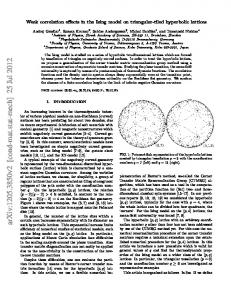
, , and observe that, for any where stands for the -fold composition of , and is the distance of from the bottom boundary of . We now describe some properties of that we use (refer to Fig. 2): is continuous and increasing , with and on . This immediately implies that has ; we denote by the at least one fixed point in least fixed point. Since is the least fixed point and then clearly , where is the derivative of . We also note that when , which corresponds to the fact that for the -boundary and the above regime of , the spin at the root is at least as likely to be as . Now, since is monotonically increasing and is converges the least fixed point of , clearly to from below, i.e., for every . 10
Proceedings of the 44th Annual IEEE Symposium on Foundations of Computer Science (FOCS’03) 0272-5428/03 $17.00 © 2003 IEEE
The first ingredient is a spatial mixing condition for in Section 3. entropy, analogous to
J(a) a
0 a 0
Definition 5.1 [Entropy Mixing] We say that satisfies if for every , any and any , non-negative function that does not depend on the following holds: In similar fashion to Theorem 3.2, if holds for sufficiently small (actually for a suitable constant ), then is bounded away from 0. To state this theorem, define , where ranges over ; i.e., is the minimum probability of any spin value at any site with any boundary condition. It is easy to see that , a constant depending only on .
1
Figure 2. Curve of the function for and . The point is the smallest fixed point of .
Theorem 5.2 For any and , if satisthen fies for all . In particular, if with the above parameters holds for some fixed and , for with fixed and an arbitrary full subtree, all then .
for , and the funcThus, since tion is monotonically increasing in the interval , for every . What remains to be shown is that . This follows from the fact that , together with the following lemma: Lemma 4.6 Let Then
be any .
Proof: From the definitions of
fixed and
point
of
This theorem is proved in exactly the same way as Theorem 3.2, via the following intermediate condition analogous to that in Lemma 3.3:
.
, if Lemma 5.3 For any then for every , any fies any function , the projected entropy is bounded above by
we have:
where
satisand
.
Starting from this condition, the proof proceeds exactly as in Section 3, under the syntactic substitution of by . Note that the only properties of that we used were (3), (4) and (5), which also hold for . in The second ingredient is the verification of the situations of interest. Perhaps surprisingly, it turns out that this can be reduced to essentially the same condition on the quantities and from Definition 4.2 as we used for the spectral gap. Specifically, we get the following analog of Theorem 4.3:
This completes the proof of Theorem 4.1 part (ii).
5 The log-Sobolev constant In this section we indicate how to extend the machinery of Sections 3 and 4 to the log-Sobolev constant , proving that it too, like , is in all the scenarios we have analyzed. By Theorem 2.1 this improves to , and our mixing time bounds from hence verifies Theorems A and B of the Introduction. Though technically slightly more involved, our analyfollows conceptually very similar lines to that sis of ; we therefore only outline it here and refer the of reader to the full version [18] for the details.
satisTheorem 5.4 Any Gibbs distribution for all , where , fies and are the constants associated with the seas specified in Definition 4.2, and is quence a constant that depends only on . In particular, if then there exists a constant such that, for every , the measure satisfies for all , and hence . 11
Proceedings of the 44th Annual IEEE Symposium on Foundations of Computer Science (FOCS’03) 0272-5428/03 $17.00 © 2003 IEEE
Remark: We should note that the above machinery, like its
[6] P. B LEHER , J. R UIZ and V. Z AGREBNOV, “On the purity of the limiting Gibbs state for the Ising model on the Bethe lattice,” J. Stat. Phys. 79 (1995), pp. 473–482. [7] T. B ODINEAU and F. M ARTINELLI, “Some new results on the kinetic Ising model in a pure phase,” J. Stat. Phys. 109 (1), 2002. [8] F. C ESI, “Quasi-factorization of the entropy and logarithmic Sobolev inequalities for Gibbs random fields,” Probab. Theory Related Fields 120 (2001), pp. 569–584. [9] W. E VANS , C. K ENYON , Y. P ERES and L.J. S CHULMAN , “Broadcasting on trees and the Ising model,” Ann. Appl. Probab. 10 (2000), pp. 410–433. [10] D. F ISHER and D. H USE, “Dynamics of droplet fluctuations in pure and random Ising systems,” Physics Review B 35 (13), 1987. [11] H.-O. G EORGII, Gibbs measures and phase transitions, de Gruyter Studies in Mathematics 9, Walter de Gruyter & Co., Berlin, 1988. [12] D. I OFFE, “A note on the extremality of the disordered state for the Ising model on the Bethe lattice,” Letters in Mathematical Physics 37 (1996), pp. 137–143. [13] J. J ONASSON and J.E. S TEIF, “Amenability and phase transition in the Ising model,” J. Theoret. Probab. 12 (1999), pp. 549–559. [14] R. LYONS, “Phase transitions on non amenable graphs,” J. Math. Phys. 41 (2000), pp. 1099–1127. [15] F. M ARTINELLI, “Lectures on Glauber dynamics for discrete spin models,” Lectures on Probability Theory and Statistics (Saint-Flour, 1997), Lecture notes in Mathematics 1717, pp. 93–191, Springer, Berlin, 1998. [16] F. M ARTINELLI and E. O LIVIERI, “Approach to equilibrium of Glauber dynamics in the one phase region I: The attractive case,” Comm. Math. Phys. 161 (1994), pp. 447–486. [17] F. M ARTINELLI , E. O LIVIERI and R. S CHONMANN , “For 2-D lattice spin systems weak mixing implies strong mixing,” Comm. Math. Phys. 165 (1994), pp. 33–47. [18] F. M ARTINELLI , A. S INCLAIR and D. W EITZ, “The Ising model on trees: Boundary conditions and mixing time,” Tech. Report UCB//CSD-031256, Dept. of EECS, UC Berkeley, July 2003. http://sunsite.Berkeley.EDU/NCSTRL/ [19] F. M ARTINELLI , A. S INCLAIR and D. W EITZ, “Fast mixing for independent sets, colorings and other models on trees,” preprint, 2003. [20] Y. P ERES and P. W INKLER , personal communication. [21] C.J. P RESTON , Gibbs states on countable sets, Cambridge Tracts in Mathematics 68, Cambridge University Press, London, 1974. [22] L. S ALOFF -C OSTE, “Lectures on finite Markov chains,” Lectures on probability theory and statistics (Saint-Flour, 1996), Lecture notes in Mathematics 1665, pp. 301– 413, Springer, Berlin, 1997. [23] D.W. S TROOCK and B. Z EGARLINSKI, “The logarithmic Sobolev inequality for discrete spin systems on a lattice,” Comm. Math. Phys. 149 (1992), pp. 175–194.
counterpart for the spectral gap, holds for any spin system on a tree, as explained in the companion paper [19].
Since in Section 4.2 we already calculated and for the Ising model in the ranges of parameters in Theorems A and B, and showed that in both cases , we immediately get that in both cases. In light of Theorem 2.1, this completes our proof of Theorems A and B. We conclude with a few words about the proof of Theorem 5.4. The essential difference between this proof and that of Theorem 4.3 is revealed in Claim 4.4. In part (i) of that claim, we bounded the expected after going levels Hamming distance . In fact, by relating the downdown the tree by ward coupling to a super-critical branching process, we can prove that the Hamming distance is not much larger than this expected value with very high probabil, ity; specifically, we can prove that, for every
where as above. Using this strong concentration of the Hamming distance, we can then analogous to our bound obtain a bound on on in Theorem 4.3. This argument is spelled out in detail in the full version [18].
Acknowledgments We thank Elchanan Mossel and Yuval Peres for useful discussions about reconstruction on trees and related topics.
References [1] D. A LDOUS, “Random walks on finite groups and rapidly mixing Markov chains,” S´eminaire de Probabilites XVII, Lecture Notes in Mathematics 986, pp. 243–297, Springer, Berlin, 1983. [2] R.J. B AXTER , Exactly solved models in statistical mechanics, Academic Press, London, 1982. [3] N. B ERGER , C. K ENYON , E. M OSSEL and Y. P ERES, “Glauber dynamics on trees and hyperbolic graphs,” preprint, 2003. Preliminary version: C. K ENYON , E. M OSSEL and Y. P ERES, “Glauber dynamics on trees and hyperbolic graphs,” Proc. 42nd IEEE Symposium on Foundations of Computer Science (2001), pp. 568–578. [4] L. B ERTINI , N. C ANCRINI and F. C ESI, “The spectral gap for a Glauber-type dynamics in a continuous gas,” Ann. Inst. H. Poincar´e Probab. Statist. 38 (2002), pp. 91–108. [5] P. B LEHER , J. R UIZ , R.H. S CHONMANN , S. S HLOSMAN and V. Z AGREBNOV, “Rigidity of the critical phases on a Cayley tree,” Moscow Math. J. 1 (2001), pp. 345–363.
12 Proceedings of the 44th Annual IEEE Symposium on Foundations of Computer Science (FOCS’03) 0272-5428/03 $17.00 © 2003 IEEE