This paper shows that unless the price change between these two dates is taken into account, the CPI ceases to be a proper statis- tical price index of the ...
The Laspeyres bias in the Spanish consumer price index J . R U I Z - C A S TI L LO , E . L E Y * and M . I Z Q U I E R D O z Dept. de EconomõÂa, Universidad Carlos III de Madrid, Spain, *IMF Institute, Washington DC, USA and zFEDEA and Bank of Spain, Madrid, Spain
The CPI compares the cost of acquiring a reference quantity vector at current and base prices. Such reference vector is the vector of mean quantities actually bought by a reference population, whose consumption patterns are investigated during a period ½ prior to the index base period 0. This paper shows that unless the price change between these two dates is taken into account, the CPI ceases to be a proper statistical price index of the Laspeyres type. Among several negative consequences, the most important is that this omission produces a bias in the measurement of in¯ation: the `Laspeyres bias’. Using Spanish data, the size of the Laspeyres bias is estimated at ¡0.061% per year, during 1992±1998. The Laspeyres bias in shorter time periods reached ¡0.122% per year in 1992, and ¡0.108 in 1997.
I. INTRODUCTION A true Cost of Living Index (or COLI for short) for an individual consumer compares a vector of current prices with a given vector of base prices while maintaining constant the consumer’s living standard or utility level. Whilst the consumer’s preferences would need to be known in order to estimate a COLI, a Statistical Price Index (SPI for short) serves the same purpose but maintains constant a reference quantity vector which, in principle, can be directly observed. When the utility level or the quantity vector correspond to the base period, we say that the COLI or the SPI are of the Laspeyres type. In this case, the (observable) Laspeyres SPI provides an upper bound to the (conceptually appealing) Laspeyres COLI (KonuÈs, 1924). In practice, o cial statistical agencies are concerned with group indexes which are meant to be representative of a certain population of households (individuals or consumers). Consumers’ behaviour is investigated by means of a household budget survey. On the basis of this information, a Consumer Price Index (CPI) ± which is an aggregate SPI where the reference the vector is the one of mean quantities actually bought by the reference population ±
can then be constructed. However, because the survey’s collection period typically precedes the base period, statistical o ces must properly take into account the price change between these two dates. In those countries where this is done, the CPI becomes what has been called a modi®ed Laspeyres SPI (Moulton, 1996). Such a CPI is a weighted average of a set of household-speci®c CPIs in which each household’s reference quantity vector is the one she acquired during the survey period. The connection between each individual’s CPI and a modi®ed Laspeyres COLI provides the basis for a normative rationale for the CPI. This paper is concerned with those countries where statistical o ces do not make any adjustment in the CPI weights for the price change between the survey’s collection period and the base period. It is important to emphasize that those countries which conduct a yearly household survey in order to construct a chained-Laspeyre s price index can also be a ected by this problem. As pointed out by Fry and Pashardes (1986), the weights used in the UK Retail Price Index correspond to expenditures incurred, on average, 12 months prior to the base change which takes place in January of every year. Since, at the time, the price changes occurred during these 12 months were not taken into account to express the weights at base prices, the UK chained-price index was not a group index of the Laspeyres type. 1
The US, Germany, France, UK and many OECD countries presently correct for this problem. However, together with Spain, among the countries which change the base after a number of years, Argentina and Austria (for detailed products) su er the problem. Among the countries with a yearly chained price index, in Norway the base period has a six month lag relative to the aggregate weights which are estimated as a three year average. On the other hand, many non-OECD countries ± like Colombia, Chile, Denmark and Peru ± have recently made the necessary methodological changes to correct the problem. Those countries which do not take fully into account the price change between the survey’s collection period and the base period face three di culties: (1) The nexus between an individual CPI and a COLI breaks down and, with it, the basis for a normative justi®cation of the aggregate CPI. (2) The individual CPIs are no longer valid for expressing household total expenditures in the survey period at the constant prices of some other period. (3) Using a wrong group index of this type, rather than a true modi®ed Laspeyres SPI, creates what we call a Laspeyres bias in the measurement of in¯ation. The sign of this bias is empirically related to the plutocratic gap, namely, the bias in the measurement of in¯ation which appears when we use the present plutocratic CPI rather than a democratic one in which all households receive the same weight ± see Izquierdo et al. (2002) and Ley (2002). In Spain, the household budget surveys which serve to estimate the weights (or the reference quantity vector) of the o cial CPI are the EPFs (Encuestas de Presupuestos Familiares), conducted by the INE (Instituto Nacional de EstadõÂstica). This paper constructs a series of modi®ed Laspeyres indexes for each household interviewed in each of the two latest EPFs. These surveys, gathered in 1980±1981 and 1990±1991, have been used in the CPI systems based in 1983 and 1992, respectively. The main empirical results are that for the two periods 1983 to December 1992, and 1992 to January 1998, the Laspeyres bias is equal to ¡0:026 and ¡0:061, respectively. Thus, during the last 12 years the o cial Spanish CPI has been (slightly) underestimating the in¯ation which would have been observed if the true modi®ed Laspeyres price indexes has been used. The rest of the paper is organized into three Sections. Section II introduces the notation for individual and group indexes. Section III presents the empirical results, while Section IV concludes. Some data details are relegated to an Appendix.
II. INDIVIDUAL AND GROUP PRICE INDEXES Let there be N goods and H households indexed by i ˆ 1; . . . ; N and h ˆ 1; . . . ; H, respectively, and let 1 q ˆ …q1 ; . . . ; qN † be a commodity vector. Each household h h is characterized by her total expenditures, x , and her preferences represented by a utility function U h …q†. Assume that all households have the same preferences, so that u ˆ U h …q† ˆ U …q† for all h, and let c…u; p†, be the cost or expenditure function, which gives the minimum cost of achieving the utility level u at prices p. Under general conh h h ditions, it is known that x ˆ c…U …q †; p†, where q is the utility maximizing commodity vector at prices p when h household expenditures are x . Consider two price vectors p0 and pt in periods 0 and t. A true or a Kon us COLI for each household which takes as h reference the utility level u , is de®ned as the ratio of the minimum cost of achieving that utility level at prices pt and h h h p0 : µ…pt ; p0 ; u † ˆ c…pt ; u †=c…p0 ; u †. When the reference utility is the utility maximizing level at prices p0 , denoted h h by u0 , it is said that the COLI µ…pt ; p0 ; u0 † is a Laspeyres h type index. Given a reference commodity vector, q , a SPI h is de®ned as the ratio of the cost of acquiring q at prices pt 2 h h h h h and p0 : `…pt ; p0 ; q † ˆ pt ¢ q =p0 ¢ q . When q ˆ q0 , the utility maximizing vector at prices p0 , it is said that the SPI h `…pt ; p0 ; q0 † is a Laspeyres type index. A fundamental theorem in KonuÈs (1924) establishes that, under general assumptions, the Laspeyres SPI provides an upper bound to the Laspeyres COLI, i.e., if h h h h u0 ˆ U …q0 †, then µ…pt ; p0 ; u0 † µ `…pt ; p0 ; q0 †. Equality is obtained when preferences are of the Leontief type, i.e., when there is no substitution between goods.
The modi®ed Laspeyres CPI De®ne the vector P of mean quantities q0 ˆ …q10 ; . . . ; qI0 †, h where q·i0 ˆ …1=H † h qi0 . The aggregate Laspeyres SPI is de®ned as follows: `…pt ; p0 ; ·q0 † ˆ
pt ¢ ·q0 p0 ¢ ·q0
…1 †
However, the CPI actually computed by statistical agencies is not exactly an aggregate Laspeyres SPI of the type de®ned in Equation 1. The reason is that individual behaviour is typically investigated by means of a household budget survey conducted in a period ½ prior to the index base period, say period 0.
1
A few words on the notation; superscripts will be used for households, and subscripts P for goods and time. Boldface symbols will be used to denote vectors, and the `¢’ operator willPindicate a vector inner product: p ¢ q ˆ i pi qi . 2 h h h De®ning the budget shares P h wi ˆ pi0 qi = i pi0 qi , an SPI can also be conveniently expressed as a weighted sum of individual price h changes: `…pt ; p0 ; q † ˆ i wi …pit =pi0 †. 2
p y
p
Household budget surveys provide information on inh dividual expenditures in each good, xi½ , and on total expenh ditures, x½ , not on individual prices and quantities ± which are often hard to de®ne. Under the assumption that all households living in the same area face the same prices, observable household expenditures on item i by household h living in area j can also be viewed as the product of a price, pij½ , and a quantity, qhi½ , ± i.e., xhi½ ˆ pij½ qhi½ . When holding information on the prices at ½ , pij½ , quantities purh h chased can then be recovered for each good, qi½ ˆ xi½ =pij½ , 3 and ·q½ used in the index construction instead of ·q0 . In this setting, the CPI based in period 0 is an aggregate SPI de®ned as: p ¢ ·q q † ` …p ; p ; · CPIt ² `…pt ; p0 ; ·q½ † ˆ t ¢ ½ ˆ … t ½ ½ † p0 ·q½ ` p0 ; p½ ; ·q½
…2†
This is what the BLS calls a modi®ed Laspeyres aggregate price index (Moulton, 1996), with base period 0 and reference consumption patterns surveyed at ½. For each household h: cpith ² `…pt ; p0 ; qh½ † ˆ
h pt ¢ q½ p0 ¢ qh½
ˆ
h `…pt ; p½ ; q½ † `…p0 ; p½ ; qh½ †
De®ne, for each household h the plutocratic weight: h 1 p0 ¢ q½ h ¿ ˆ H p0 ¢ ·q½
Then, as known from Prais (1958): P X X p ¢ qh p ¢ qh …1=H † ¢ h ¢ q½ h h ˆ 1 0 h pt q½ ˆ pt · ½ t ½ ˆ ¿ cpit h ¢ ¢ ¢ q½ ¢ p q H p q p · · p q 0 0 0 · ½ ½ 0 ½ h h ˆ CPIt
…3†
Thus, on one hand, the CPI is an SPI which serves to compare the price vector in any period t with the price vector in the base period 0, while maintaining constant the aggregate vector ·q½ of mean quantities actually purchased during the survey period ½ ± see Equation 2. On the other hand, the CPI is the plutocratic weighted mean of a set of household-speci®c modi®ed Laspeyres price indexes ± see Equation 3. The question is, what is the normative basis for such a construction? To answer this question it is necessary to de®ne a set of household-speci®c modi®ed Laspeyres COLIs. For each h, let uh½ ˆ U …qh½ †. It is easy to see that the ratio of the corresponding Laspeyres COLIs leads to what is called a modi®ed Laspeyres COLI: h µ…pt ; p½ ; u½ † µ…p0 ; p½ ; uh½ †
ˆ
h c…pt ; u½ † c…p0 ; uh½ †
ˆ µ…pt ; p0 ; uh½ †
h KonuÈ s theorem ensures that, for each h, `…ps ; p½ ; q½ † ¡ h µ…ps ; p½ ; u½ † ¶ 0 for s ˆ 0; t, but it says nothing about the ratio of the Laspeyres indexes which give rise to an individual CPI. However, the household budget survey collection period ½ is typically not far apart from the base year 0 of the CPI system. Thus, under the assumption h h that the substitution bias `…p0 ; p½ ; q½ † ¡ µ…p0 ; p½ ; u½ † is h h smaller than `…pt ; p½ ; q½ † ¡ µ…pt ; p½ ; u½ †, a household-speci ®c CPI provides an upper bound to a modi®ed Laspeyres COLI. P In view of Equation 3, it is seen that h h CPIt ¶ h ¿ µ…pt ; p0 ; q½ †. Thus, only under the assumption that for a su ciently large number of households: h h ` …p t ; p ½ ; q ½ † ¶ µ …p t ; p ½ ; u ½ † ˆ … h h cpit ˆ µ pt ; p0 ; u½ † h `…p0 ; p½ ; q½ † µ…p0 ; p½ ; uh½ †
the aggregate CPI provides an upper bound to a plutocratic weighted mean of modi®ed Laspeyres COLIs. The Spanish CPI In Spain, the INE does not use information on the prices pij½ when constructing its price index. Therefore, only an IPC (Indice de Precios de Consumo) can be de®ned. At the individual level, for any household h, the individual IPC is de®ned as: P X X p qh p … † h i½ i½ it ˆ P i pit pi½ =pi0 qi½ h ² h pit ˆ ipct wi½ … † h ¢ h pi0 i pi0 pi½ =pi0 qi½ i i p½ q½ pi0 P h ¢ gh ˆ P i pit ²i ˆ pt ˆ `…pt ; p0 ; gh † …4 † h p0 ¢ gh i pi0 ²i
h h h where wi½ ˆ xi½ =x½ is the expenditure weight of good i, and h h h g ˆ …²1 ; . . . ; ²N † with:
pi½ h h qi½ ²i ˆ pi0
…5 †
Thus, the Spanish IPC for each h is a SPI where the reference vector gh is the vector qh multiplied by the price change between period ½ and period 0. At the aggregate level, let g · be the average P h reference vector with generic element ²·i ˆ …1=H † h ²i . Then, the aggregate IPC is given by: p ¢g · IPCt ² `…pt ; p0 ; ·g† ˆ t ¢ g p0 ·
…6 †
De®ne now the plutocratic weights: h h h 1 p0 ¢ g ˆ 1 p½ ¢ q½ ˆ Px½ h ¿½ ˆ h H p0 ¢ g H p½ ¢ q½ · h x½
3
For simplicity, in what follows geographical details will be ignored and the subindex j dropped. However, it should be kept in mind throughout that statistical agencies gather prices by geographical areas and, therefore, all formulas should re¯ect this ± see, for example, Izquierdo et al. (2002). 3
Then, again it is seen that: IPC t ˆ
X
h
h
¿½ ipct
h
…7†
That is, on one hand, the IPC for the population as a whole is an aggregate SPI which takes ·g as the reference vector, which is the vector of mean quantities actually purchased in period ½ multiplied by the price change between period ½ and period 0 ± see Equation 6. On the other hand, the general IPC is the plutocratic weighted mean of the household±speci®c IPCs ± see Equation 7. This construction poses, at least, three problems. In the h ®rst place, at the individual level the index ipct is unrelated h† … to the modi®ed COLI µ pt ; p0 ; u½ . Consequently, the normative basis for the aggregate IPCt is lost. In the second place, suppose that it is wished to establish whether, for example, mean household expenditures have risen or not in real terms between period ½ and period 1 H t > 0. Denote by x½;t ˆ …x½;t ; . . . ; x½;t † the distribution of household expenditures in period ½ at prices of period t, where for each household xh½;t ˆ xh½ µ…pt ; p½ ; uht †. The change in mean household expenditures at prices pt can be expressed as ¢…pt † ˆ ·…xt † ¡ ·…x½;t †, where ·…x† denotes the mean of distribution x. Similarly, the change in mean household expenditures at prices of period ½ can be expressed as ¢…p½ † ˆ ·…xt;½ † ¡ ·…x½ †. If there is a proper household-speci®c Laspeyres price index for each h, then h h h h h x^½;t ˆ x½ `…pt ; p½ ; q½ † ˆ pt ¢ q½ ¶ x½;t can be computed for … † ¶ … † each h. Thus, · x ^ ½;t · x½;t and a lower bound can be h h h provided for ¢…pt †. Similarly, x^t;½ ˆ xt =`…pt ; p½ ; qt † ˆ h h p½ ¢ qt ¶ xt;½ can be computed for each h, and that distribution used to obtain an upper bound for ¢…p½ †. However, if there are only household-speci®c ipcht ’s, then the only thing that can be done to express the household total h expenditures in period ½ at prices pt is to multiply x½ by the index de®ned in Equation 4: ¢ gh h h h p h x½ ipct ˆ …p½ ¢ q½ † t h ˆ pt ¢ g p0 ¢ g
…8†
h However, in this operation pt ¢ q½ cannot be recovered as h desired. Similarly, with such indexes p½ ¢ qt cannot be recovered either. Hence, by this route neither a lower bound for ¢ …pt † nor an upper bound for ¢…p½ † can be provided. Finally, let ºt be the in¯ation rate according to the IPCt de®ned in Equation 7. Measuring in¯ation in this way, one incurs in some bias relative to the alternative of using a modi®ed Laspeyres group price index CPIt as de®ned in Equation 2 ± let º^t be the corresponding in¯ation rate. Then the Laspeyres bias is de®ned by …ºt ¡ º^t †. What can be expected about the sign of the Laspeyres bias in a given period? The answer depends on the behaviour of
prices during that period and during the time interval which goes from the survey’s collection period ½ to the base period 0. It has been seen that all group indexes in this section are weighted averages of the individual indexes with weights proportional to household total expenditures. Alternatively, a democratic group index can be de®ned in which all household-speci®c indexes weigh equally (Prais, 1959). The plutocratic gap in the measurement of in¯ation is then de®ned as the di erence between the in¯ation estimated according to a plutocratic and a democratic group index. When the in¯ation in a given period is greater (smaller) for the rich than for the poor households, then the plutocratic weighted mean would be greater (smaller) than the simple mean. Therefore, the plutocratic gap is expected to be positive (negative) when prices behave in an anti-rich (anti-poor) way. Suppose now that between periods ½ and 0 all prices h h have risen, so that, for each h, ²i < qi½ for all i ± see Equation 5. The greater the in¯ation experienced by a particular good i, the greater the di erence between ²hi and qhi½ . Suppose that the prices of luxuries (goods with total expenditures elasticity greater than 1) have increased by more than the price of necessities (goods with total expenditures elasticity smaller than 1); or in other words, suppose that prices have been anti-rich so that the plutocratic gap has been positive. Then, for each h, the relative importance of h h luxuries in g is less than in q½ , while the opposite will be the case for necessities. Suppose further that the same price pattern obtains between period 0 and period t, that is, suppose that prices are again anti-rich. Then, for each h, h the SPI that takes as reference the vector g would tend to understate the in¯ation which has taken place according to a modi®ed Laspeyres price index which takes the vector h q½ as reference. In this case, the Laspeyres bias would have a negative sign. On the contrary, given that it is assumed that prices are anti-rich from period ½ to period 0, if between period 0 and period t the plutocratic gap is negative, then the Laspeyres bias can be expected to be 4 positive. Nonetheless, this relationship between the Laspeyres bias and the plutocratic gap ± although it holds for the data analysed in this paper as seen below ± is not theoretically guaranteed, and it is possible to construct counterexamples when N ¶ 3.
III. EMPIRICAL RESULTS Laspeyres price indexes are constructed for all households surveyed in the two latest household surveys conducted in
h Suppose instead that from period ½ to period 0 prices are anti-poor. Then the relative importance of luxuries in g would be greater than h would be the case in q½ , while the opposite would be the case for necessities. Then the Laspeyres bias would tend to be negative (positive) according to whether prices from period 0 to period t behave in an anti-poor (anti-rich) way. 4
4
p y
p
Table 1. The Laspeyres bias (in percent per year) In¯ation Subperiods
Laspeyres bias
ºt
º^t
1980±81/83 Aug 85 to Dec 85 Dec 85 to Dec 86 Dec 86 to Dec 87 Dec 87 to Dec 88 Dec 88 to Dec 89 Dec 89 to Dec 90 Dec 90 to Dec 91 Dec 91 to Dec 92
6.896 8.217 4.622 5.895 6.908 6.589 5.576 5.364
6.852 8.230 4.587 5.866 6.923 6.641 5.603 5.486
0.033 ¡0.023 0.029 0.021 ¡0.019 ¡0.049 ¡0.037 ¡0.128
Aug 85 to Dec 92
6.848
6.867
¡0.026
5.228 4.600 4.047 3.108 2.376
5.267 4.619 4.078 3.176 2.484
¡0.039 ¡0.018 ¡0.031 ¡0.068 ¡0.108
4.120
4.181
¡0.061
Plutocratic gap
Base 1983 0.025 ¡0.157 ¡0.038 0.381 ¡0.025 ¡0.032 0.228 0.312 0.593 0.186
Base 1992 1990±91/92 Jan 93 to Jan Jan 94 to Jan Jan 95 to Jan Jan 96 to Jan Jan 97 to Jan
94 95 96 97 98
1993 to Jan 98
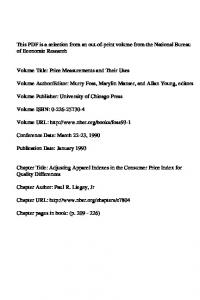
Spain from April 1990 to March 1991, and April 1980 to 5 March 1981. They are referred to as the 1990±1991 EPF, and the 1980±1981 EPF, respectively. The data sources are explained in the Appendix. Let IPCt be the group index de®ned in Equation 4 which compares the vector of prices in January of year t with the vector of prices in the base period ± for example, 0 ˆ 1983, and 1992 in the two panels of Table 1. The interannual in¯ation rate in year t is denoted by ºt ˆ ……IPCt‡1 =IPCt † ¡ 1† £ 100. Let CPIt be the modi®ed Laspeyres group index de®ned in Equation 2 referring to the same base. Denote by º^t ˆ ……CPIt =CPIt¡1 † ¡ 1† £ 100 the corresponding inter-annual in¯ation rate. The Laspeyres bias for year t is de®ned by ºt ¡ º^t . Table 1 presents the estimates for ºt , º^t and the corresponding Laspeyres bias, t ˆ 1985; . . . ; 1997. For each of the two periods 1985±1992 and 1993±1998, the Laspeyres bias is ^ , where ¦ and ¦ ^ are the average annual equal to ¦ ¡ ¦ in¯ation rates using the IPC and the CPI, respectively ± shown on the bottom row of each panel in Table 1. ~ the Denote by º~t the inter-annual in¯ation rate and ¦ average annual in¯ation rate when a democratic price P index is used to measure in¯ation, …1=H † h cpi th , instead of the plutocratic index de®ned in Equation 3. The plutocratic gap is then de®ned by ºt ¡ º~t for each year, and by
0.088 0.105 ¡0.080 ¡0.050 0.090 0.125 0.038
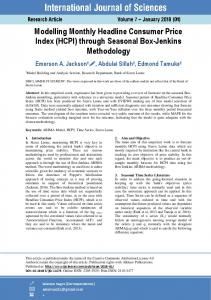
~ for the two periods 1985±1992 and 1993±1998. The ¦¡¦ estimates of the plutocratic gap are shown in the last column of Table 1. In the ®rst place, it is observed that for the 1993±1998 subperiod as a whole, the Laspeyres bias is equal to ¡0:061% per year (¡0:026 for the 1985±1992 subperiod). How can this negative sign be explained? Notice that from the 1990±1991 EPF’s collection period to the base year 1992, prices behave in an anti-rich way: the plutocratic gap is equal to 0.088% per year (0.025 from the 1980± 1981 survey period to the base year 1983). As seen in the last section, this means that the o cial IPC would tend to give less weight to luxuries and more weight to necessities than a modi®ed Laspeyres group index. On the other hand, from 1992 to January 1998 price behaviour is again antirich: the plutocratic gap is equal to 0.038% per year (0.186 from August 1985 to December 1992). Consequently, the IPC would tend to register a smaller in¯ation, ¦, than the ^ . This explains the negamodi®ed Laspeyres alternative, ¦ tive sign of the Laspeyres bias that is found on the bottom row of each panel in Table 1. To appreciate the variability of the Laspeyres bias during the entire period considered in this paper, the top panel in Figure 1 shows a series of monthly observations on the evolution of the inter-annual Laspeyres biases and
5
For the survey conducted during 1973±1974 the only information available on the in¯ation between the survey period and the base year is at a very aggregated level, ®ve goods, which does not allow us to estimate the Laspeyres bias. 5
199609 199703 199709
199609
199703
199709
199403
199309
199303
199603
-3.0
199603
-2.0 199509
-1.0
199509
0.0 199503
1.0
199503
2.0 199409
Monthly p lutocratic gap (annualized)
199409
199403
199309
199303
199209
199203
199109
199103
199009
199003
198909
198903
198809
198803
198709
198703
198609
198603
198509
Laspeyres Bias
199209
199203
199109
199103
199009
199003
198909
198903
198809
198803
198709
198703
198609
198603
198509
199709
199703
199609
199603
199509
199503
199409
199403
199309
199303
199209
199203
199109
199103
199009
199003
198909
198903
198809
198803
198709
198703
198609
198603
198509
Inter-annual Laspeyres bi as and p lutocratic gap (month by month)
0.50
0.25
0.00
-0.25
Plutocratic Gap
Monthly Laspeyres bias (annualized)
1
0.5
0
-0.5
-1
Fig. 1. The Laspeyres bias and the plutocratic gap (in per cent per year)
6
p y
p
Table 2. The Laspeyres bias vs the plutocratic gap Base year 1992 Intercept S.E. Plutocratic gap S.E. Durbin-Watson 2 R· F …1; T ¡ 2† T
3.5E-5 (1.2E-5) ¡0.1766 (0.046) 2.12 0.29 24.1 59
1983 1.6E-5 (3.0E-5) ¡0.2485 (0.035) 1.62 0.36 49.25 87
plutocratic gaps for October 1986 to January 1998. Since each annual in¯ation is a moving average of the in¯ation of the 12 previous months, the information contained on each data point overlaps signi®cantly with the adjacent observations (the series are integrated). The bottom panels show the ®rst di erences of these series ± which are nothing but monthly in¯ation biases. The monthly series have been annualized in order to facilitate its interpretation. These annualized series display very large magnitudes, reaching close to §1% per year in some instances in the 1980s. These large biases of di erent signs tend to cancel o over longer periods and inter-annual biases show smaller magnitudes. Given the anti-rich price bias from the survey’s period to the base year in the two cases considered, it is known that the o cial IPC takes as reference a vector of aggregate quantities where luxuries receive less weight and necessities receive more weight than they would in a modi®ed Laspeyres construction. Therefore, if in a given period the plutocratic gap is positive (negative), re¯ecting an anti-rich (anti-poor ) bias, then the corresponding Laspeyres bias is expected to move in the opposite direc6 tion. This is indeed what is observed in Figure 1. Table 2 shows the results of the regression of the Laspeyres bias against the corresponding plutocratic gap, using intermonthly in¯ation data. The negative relationship between the Laspeyres bias and the plutocratic gap is displayed in an estimated coe cient of about ¡0:2 with a standard error of about 0.04 for the 1992 and 1983 base systems.
IV. CONCLUSIONS The CPI compares the cost of acquiring a reference quantity vector at current and base prices. Such reference vector
is the vector of mean quantities actually bought by a reference population, whose consumption patterns are investigated during a period ½ prior to the index base period 0. This paper has shown that unless one takes into account the price change between these two dates, each component of the reference quantity vector will be multiplied by the ratio of the price of the good in period ½ and in period 0. As a consequence, the CPI ceases to be a proper SPI of the Laspeyres type. This has several negative consequences: (1) The link between the CPI and a group index based on the COLIs of the reference population breaks down; (2) the possibility of expressing the consumption expenditures in period ½ at prices of other periods disappears, and, more importantly, (3 ) it produces a bias in the measurement of in¯ation which we have called the `Laspeyres bias’. The relation of this bias with the plutocratic gap (Ley, 2002; Izquierdo et al., 2002) during a particular period t depends on whether prices exhibit an anti-rich or an anti-poor behaviour from period ½ to period 0, and from period 0 to the period t in question. In¯ation targets constitute a policy objective of paramount importance. For example, the Maastrich agreements in 1992 singled out an in¯ation objective as one of the three criteria for European Union members to become part of the European Monetary Union. Moreover, thanks to the ample publicity received by the report to the US Senate by a commission headed by Michael Boskin, it has been forcefully reminded about the dramatic economic consequences of a relatively small bias in the measurement of in¯ation ± see Boskin et al. (1996). Consequently, statistical o ces must ensure that the CPI preserves its alleged properties and that its measurement is as free as possible from any bias. Of course, the urgency of the problem at hand depends on its quantitative importance. This paper has presented some evidence on the Laspeyres bias in Spain for the CPI systems based in 1983 and 1992. It has been shown that this bias has a predominantly negative sign for an extended period of time which expands from 1985±1998. Essentially, this is explained by the overall anti-rich bias exhibited by the evolution of prices in Spain during this period. This does not preclude that the Laspeyres bias takes a positive sign during speci®c subperiods characterized by an anti-poor price behaviour. Finally, the Laspeyres bias has displayed a considerable size during certain periods of time. For instance, from 1992±1998, the size of the Laspeyres bias was 0.061% per year, or about 6% of the overall bias from ®ve sources estimated
6
In Table 3.2 of Fry and Pashardes (1986, p. 26) the importance of the Laspeyres bias can be observed in the UK. Qualitatively, the di erence with Spain is that, in the UK the bias in every year from 1977±1984 has a positive sign ± except for the period 1975±1977 in which the bias is zero or slightly negative ± reaching a maximum value of 0.8% in 1978. According to the discussion in Section II, the explanation is clear: as these authors and others have documented ± see also Crawford (1994) and Muellbauer (1974 a,b) ± during the 1970s price behaviour in the UK was anti-poor. 7
by the Boskin commission for the USA, which is equal to 7 1.1% per year. The Laspeyres bias in shorter time periods has reached 0.122, and 0.108% per year in 1992, and 1997, respectively. The practical message of the paper is clear: when the household budget survey’s collection period ½ di ers from the CPI base year 0, it is necessary to gather information on the evolution of prices from period ½ to period 0 in order to express the expenditures incurred in period ½ at base period prices. Only in this case is it possible to construct (modi®ed) Laspeyres price indexes which take as reference the mean commodity vector actually acquired by consumers during period ½ . The di culty lies in the fact that the data collected in the household budget survey is essential for deciding on the characteristics of the new base in relation to the item space, product speci®cations, and the establishments where price quotes should be taken. How is it possible to record goods prices from period ½ to period 0 according to the new methodology at the same time that such a methodology is being decided upon? Surely, some compromises should be adopted in order to ®nd an answer to this practical question. There seems to be no doubt that the statistical agency responsible for the CPI is the best prepared to carry out this task. Finally, it is worthwhile to emphasize that, once the comparison of the old and the new base is indirectly established through this process, the statistical agency is in a good position to provide the best possible reconstruction of past in¯ation according to the new methodology. This is potentially very important for those analysts in charge of predicting the short-run CPI behaviour immediately after a change of base.
A C K N O W LE D G E M E N T The authors would like to thank Mercedes Sastre for sharing her insightful ideas in numerous conversations which decisively motivated this research, also Marshall Reinsdorf for valuable comments. Financial support from ``la Caixa’’ is gratefully acknowledged.
R E F E R E N C ES CatasuÂs, V., Malo de Molina, J. L., MartõÂ nez, M. and Ortega, E. (1986) Cambio de base del Indice de Precios de Consumo, mimeo, Madrid, Banco de EspanÄa. Crawford, I. (1994) UK Household Cost-of-Living Indexes , Institute for Fiscal Studies, London. Fry, V. and Pashardes, P. (1985) The RPI and the Cost of Living, Report Series No. 22, Institute for Fiscal Studies, London.
GarcõÂ a EspanÄa, E. and Serrano, J. M. (1980) Indices de Precios de Consumo, Instituto Nacional de EstadõÂ stica, Madrid: Ministerio de EconomõÂ a y Comercio, Madrid. INE (1983) Encuesta de Presupuestos Familiares 1980±81. MetodologõÂa y resultados, Instituto Nacional de EstadõÂ stica, Madrid. INE (1985) Indice de Precios de Consumo. Base 1983. MonografõÂa TeÂcnica, Instituto Nacional de EstadõÂ stica, Madrid. INE (1992) Encuesta de Presupuestos Familiares 1990±91. MetodologõÂa, Instituto Nacional de EstadõÂ stica, Madrid. INE (1994) Indice de Precios de Consumo. Base 1992. MetodologõÂa, Instituto Nacional de EstadõÂ stica, Madrid. Izquierdo, M., Ley, E. and Ruiz-Castillo, J. (2002) The plutocratic gap in the CPI: evidence from Spain, IMF Sta Papers, forthcoming. KonuÈs, A. A. (1924) The problem of the true index of the cost of living, English version in Econometrica, 7, 10±29. Ley, E. (2002) Whose in¯ation? A characterization the CPI plutocratic gap, mimeo, available online: http://econwpa. wustl.edu/ Lorenzo, F. (1998) ModelizacioÂn de la in¯acioÂn con ®nes de prediccioÂn y diagnoÂstico, PhD Dissertation, Universidad Carlos III de Madrid, Madrid. Moulton, B. (1996) Constant elasticity cost-of-living index share relative form, mimeo, Bureau of Labour Statistics. Muellbauer, J. (1974a) Prices and inequality: the United Kingdom experience, Economic Journal, 84, 32±55. Muellbauer, J. (1974b) The political economy of price indexes, Birbeck Discussion Paper 22. Prais, S. (1958) Whose cost of living?, The Review of Economic Studies, 26, 126±34. Ruiz-Castillo, J., Higuera, C., Izquierdo, M. and Sastre, M. (1999a) Series de precios individuales para las EPF de 1973±74, 1980±81 y 1990±91 con base en 1976, 1983 y 1992, mimeo, available online: http://www.eco.uc3m.es/ investigacion/epf.html Ruiz-Castillo, J., Ley, E. and Izquierdo, M. (1999b) La MedicioÂn de la In¯acioÂn en EspanÄa, la Caixa, Barcelona.
APPENDIX: THE CONSTRUCTION OF H O U S E H O L D - S P E C I F I C L A S P EY R E S S P I s In order to construct a series of household-speci ®c Laspeyres price indexes for a given period, the following three pieces of information are needed: (1) The household budget survey which serves to estimate the aggregate weights of the o cial CPI; (2) a set of price subindexes for the period in question at a certain level of commodity and spatial disaggregation ; and (3) a set of estimated price changes ± that shall be called `adjustment factors’ ± between the survey collection period ½ and the o cial base period 0. In the Spanish case, Laspeyres price indexes are constructed for all households surveyed in the two latest EPFs gathered in 1990±1991 and 1980±1981, respectively. These are large comparable samples consisting of 21 155,
7
In Ruiz-Castillo et al. (1999b) it is estimated that this overall bias in Spain is of the order of 0.60% per year. Thus, the Laspeyres bias during the 1990s is about 10% of our best estimate of the overall bias in the Spanish economy. 8
p y
p
and 23 972 household sample points, respectively. These samples represent a population of, approximately, 11 or 10 million households and 38 or 37 million persons, respectively, occupying residential housing in all of Spain. People living in collective housing, such as residences for the aged, hospitals, prisons, hotels, and the like, are excluded from the EPFs. The two surveys cover household expenditures on 893, and 614 commodities, respectively. In this and other respects, the later the survey period the more complete the survey is. However, they all share the same sample strati®cation design, and the same methodology to investigate household expenditures: all household members of 14 or more years of age are supposed to record all expenditures that take place during the sample week; then, in-depth interviews are conducted to register past expenditures over reference periods beyond a week and up to a year ± for further details, see INE (1992), and INE (1983). From this information the statistical o ce estimates annual expenditures on all goods. As indicated in the text, these EPFs have been used to estimate the corresponding aggregate weights of the Spanish IPC systems based in 1992 and 1983. The information on price subindexes and adjustment factors is best treated separately for each period.
The 1992 IPC: from January 1993 until the present The INE collects elementary price indexes for a commodity basket consisting of 471 items in each of 52 provinces. For con®dentiality reasons, the INE does not publish this information at the maximum spatial disaggregation level. Instead, from January 1993 it publishes on a monthly basis price subindexes for a commodity breakdown of 110 subclases, 57 ruÂbricas, 33 subgrupos and 8 grupos at the national level, the ruÂbricas, subgrupos and grupos at the 18 Autonomous Communities level, and the subgrupos and grupos at the 52 provincial level ± for further details, see INE (1994). For any commodity breakdown, it is possible to reconstruct the o cial IPC series using an appropriatel y de®ned vector of aggregate weights or budget shares. Similarly, de®ning a budget share vector for every household in the 1990±1991 sample, obtain a series of household speci®c IPCs can be obtained for any commodity breakdown. In principle, the only di erence between alternative speci®cations of the commodity space, is that the dispersion of the set of individual IPCs should be greater the greater the disaggregation level of the price information used in their construction. Unfortunately, in spite of using the same informational basis as the INE ± namely, the 1990±1991 EPF ± some small discrepancies are found between our
estimates of the aggregate budget share vectors and those published by the INE. Thus, the CPI series which can be reconstructed varies slightly depending on the di erent commodity breakdowns characterizing the price information used ± for an analysis of these discrepancies see RuizCastillo et al. (1999a). In Ruiz-Castillo et al. (1999b), it is found that the speci®cation consisting of the 21 food ruÂbricas at the Autonomous Community level, and the 32 nonfood subgrupos at the provincial level outperforms the rest of the alternatives according to various statistical and economic criteria. It should be emphasized that our series of householdspeci®c price indexes de®ned over this 53 commodity space di ers from the series underlying the o cial IPC. The reason is that there are a number of aspects in the o cial de®nition of total household expenditures for which what is believed to be superior alternatives are used: (1) the de®nition of housing expenditures for households occupying non-rental housing; (2) the inclusion of imputations for home production, wages in kind and subsidized meals, and (3) the estimation of annual food and drink expenditures using all the available information on 8 bulk purchases in the 1990±1991 EPF. As pointed out in Section II, because the INE does not use any adjustment factors for taking into account the price change between the EPF’s collection period and the base period, the o cial index `…pt ; p0 ; ·g† does not coincide with the modi®ed Laspeyres index `…pt ; p0 ; ·q½ †. Fortunately, the analysts devoted to short run forecasting of the economy need su ciently long price series drawn with a common methodology in order to do their work. Thus, when there is a change of base in the system they estimate the price changes …pit =pi0 †, with t < 0, where the commodity space, as well as the item speci®cations correspond, as best as possible, to the methodology of the new CPI base. Taking into account the methodological changes adopted by the INE for the current IPC base of 1992, Lorenzo (1998) provides such information on a monthly basis for the 110 subclases, at the national level from January 1983 until 1992. For each of the quarters (½ ˆ Spring, Summer, Autumn of 1990, and Winter of 1991), using Lorenzo (1998) data on the adjustment factors pi½ =pi0 for each of the 110 subclases the price ratios pit =pi½ ˆ …pit =pi0 †=…pi½ =pi0 † are computed, where pit =pi0 are the price subindexes provided by the INE on a monthly basis from January 1993 to January 1998. Given the Laspeyres h indexes `…pt ; p½ ; q½ †, a series of modi®ed Laspeyres price indexes is constructed from January 1993 until January 1998, based in that period 0 ˆ 1992, which takes as referh ence the commodity vector q½ actually acquired during the interview quarter ½ .
8
The joint impact of these modi®cations is important: according to Izquierdo et al. (2002), the o cial CPI understates the true Spanish in¯ation from 1992 to January of 1998 by 0.241% per year. 9
The 1983 IPC: from August 1985 to December 1992 The INE collects elementary price indexes for a commodity basket consisting of 428 items in each of 52 provinces. It publishes on a monthly basis price subindexes for a commodity breakdown of 106 subclases, 57 ruÂbricas, 29 subgrupos and 8 grupos at the national level. Complete information at the Autonomous Communities level is only available for the eight grupos ± for further details see INE (1985). The information is used for the 106 subclases at the national level. This case does not depart from the o cial de®nition of household total expenditures it agrees with the way nonrental housing is treated. Nevertheless, there are some discrepancies between the o cial aggregate weights published by the INE and those presented here. In the ®rst place, the information on all households interviewed in the 1980± 1981 EPF is used, while the INE restricts itself to a reference population which excludes single-person households
and those multi-person ones with total income below the 1980Ð1981 minimum wage or above a certain amount. These restrictions mean that the o cial IPC refers to 79% of all households, 86% of all persons, and 85% of all household expenditures. In the second place, even when this factor is taken into account, some minor discrepancies are found, as before, between our estimates of the aggregate weights and those published by the INE ± for an analysis of these discrepancies see Ruiz-Castillo et al. (1999a). As far as the adjustment factors, pi½ =pi0 , the monthly series for 60 goods is used at the national level provided by Catasu s et al. (1986) from January 1978 to July of 1985. A set of 52 goods is worked with which constitute the minimum common denominator between the 57 o cial ruÂbricas and the 60 goods in CatasuÂs (1986) ± for the details of this construction see Ruiz-Castillo et al. (1999a).
10