The Lazy Flipper: MAP Inference in Higher-Order Graphical Models by

The Lazy Flipper: MAP Inference in Higher-Order Graphical Models by Depth-limited Exhaustive Search

arXiv:1009.4102v1 [cs.DS] 21 Sep 2010

Bj¨ orn Andres, J¨ org H. Kappes, Ullrich K¨othe and Fred A. Hamprecht HCI, IWR, University of Heidelberg http://hci.iwr.uni-heidelberg.de, [email protected]

Abstract. This article presents a new search algorithm for the NP-hard problem of optimizing functions of binary variables that decompose according to a graphical model. It can be applied to models of any order and structure. The main novelty is a technique to constrain the search space based on the topology of the model. When pursued to the full search depth, the algorithm is guaranteed to converge to a global optimum, passing through a series of monotonously improving local optima that are guaranteed to be optimal within a given and increasing Hamming distance. For a search depth of 1, it specializes to Iterated Conditional Modes. Between these extremes, a useful tradeoff between approximation quality and runtime is established. Experiments on models derived from both illustrative and real problems show that approximations found with limited search depth match or improve those obtained by state-of-the-art methods based on message passing and linear programming.

1

Introduction

Energy functions that depend on thousands of binary variables and decompose according to a graphical model [1,2,3,4] into potential functions that depend on subsets of all variables have been used successfully for pattern analysis, e.g. in the seminal works [5,6,7,8]. An important problem is the minimization of the sum of potentials, i.e. the search for an assignment of zeros and ones to the variables that minimizes the energy. This problem can be solved efficiently by dynamic programming if the graph is acyclic [9] or its treewidth is small enough [3], and by finding a minimum s-t-cut [6] if the energy function is (permutation) submodular [10,11]. In general, the problem is NP-hard [10]. For moderate problem sizes, exact optimization is sometimes tractable by means of Mixed Integer Linear Programming (MILP) [12,13]. Contrary to popular belief, some practical computer vision problems can indeed be solved to optimality by modern MILP solvers (cf. Section 5). However, all such solvers are eventually overburdened when the problem size becomes too large. In cases where exact optimization is intractable, one has to settle for approximations. While substantial progress has been made in this direction, a deterministic non-redundant search algorithm that constrains the search space based on the topology of the graphical model has not been proposed before. This article presents a depth-limited exhaustive search algorithm, the Lazy Flipper, that does just that.

2

B. Andres et al.

The Lazy Flipper starts from an arbitrary initial assignment of zeros and ones to the variables that can be chosen, for instance, to minimize the sum of only the first order potentials of the graphical model. Starting from this initial configuration, it searches for flips of variables that reduce the energy. As soon as such a flip is found, the current configuration is updated accordingly, i.e. in a greedy fashion. In the beginning, only single variables are flipped. Once a configuration is found whose energy can no longer be reduced by flipping of single variables, all those subsets of two and successively more variables that are connected via potentials in the graphical model are considered. When a subset of more than one variable is flipped, all smaller subsets that are affected by the flip are revisited. This allows the Lazy Flipper to perform an exhaustive search over all subsets of variables whose flip potentially reduces the energy. Two special data structures described in Section 3 are used to represent each subset of connected variables precisely once and to exclude subsets from the search whose flip cannot reduce the energy due to the topology of the graphical model and the history of unsuccessful flips. These data structures, the Lazy Flipper algorithm and an experimental evaluation of state-of-the-art optimization algorithms on higher-order graphical models are the main contributions of this article. Overall, the new algorithm has four favorable properties: (i) It is strictly convergent. While a global minimum is found when searching through all subgraphs (typically not tractable), approximate solutions with a guaranteed quality certificate (Section 4) are found if the search space is restricted to subgraphs of a given maximum size. The larger the subgraphs are allowed to be, the tighter the upper bound on the minimum energy becomes. This allows for a favorable tradeoff between runtime and approximation quality. (ii) Unlike in brute force search, the runtime of lazy flipping depends on the topology of the graphical model. It is exponential in the worst case but can be shorter compared to brute force search by an amount that is exponential in the number of variables. It is approximately linear in the size of the model for a fixed maximum search depth. (iii) The Lazy Flipper can be applied to graphical models of any order and topology, including but not limited to the more standard grid graphs. Directed Bayesian Networks and undirected Markov Random Fields are processed in the exact same manner; they are converted to factor graph models [14] before lazy flipping. (iv) Only trivial operations are performed on the graphical model, namely graph traversal and evaluations of potential functions. These operations are cheap compared, for instance, to the summation and minimization of potential functions performed by message passing algorithms, and require only an implicit specification of potential functions in terms of program code that computes the function value for any given assignment of values to the variables. Experiments on simulated and real-world problems, submodular and nonsubmodular functions, grids and irregular graphs (Section 5) assess the quality of Lazy Flipper approximations, their convergence as well as the dependence of the runtime of the algorithm on the size of the model and the search depth. The results are put into perspective by a comparison with Iterated Conditional Modes (ICM) [5], Belief Propagation (BP) [9,14], Tree-reweighted BP [15,4] and a Dual Decomposition ansatz using sub-gradient descent methods [16,17].

The Lazy Flipper

2

3

Related Work

The Lazy Flipper is related in at least four ways to existing work. First of all, it generalizes Iterated Conditional Modes (ICM) for binary variables [5]. While ICM leaves all variables except one fixed in each step, the Lazy Flipper can optimize over larger (for small models: all) connected subgraphs of a graphical model. Furthermore, it extends Block-ICM [18] that optimizes over specific subsets of variables in grid graphs to irregular and higher-order graphical models. Naive attempts to generalize ICM and Block-ICM to optimize over subgraphs of size k would consider all sequences of k connected variables and ignore the fact that many of these sequences represent the same set. This causes substantial problems because the redundancy is large, as we show in Section 3. The Lazy Flipper avoids this redundancy, at the cost of storing one unique representative for each subset. Compared to randomized algorithms that sample from the set of subgraphs [19,20,21], this is a memory intensive approach. Up to 8 GB of RAM are required for the optimizations shown in Section 5. Now that servers with much larger RAM are available, it has become a practical option. Second, the Lazy Flipper is a deterministic alternative to the randomized search for tighter bounds proposed and analyzed in 2009 by Jung et al. [19]. Exactly as in [19], sets of variables that are connected via potentials in the graphical model are considered and variables flipped if these flips lead to a smaller upper bound on the sum of potentials. In contrast to [19], unique representatives of these sets are visited in a deterministic order. Both algorithms maintain a current best assignment of values to the variables and are thus related with the Swendsen-Wang algorithm [20,22] and Wolff algorithm [21]. Third, lazy flipping with a limited search depth as a means of approximate optimization competes with message passing algorithms [14,23,24,4] and with algorithms based on convex programming relaxations of the optimization problem [24,25,26,27], in particular with Tree-reweighted Belief Propagation (TRBP) [15,4,28] and sub-gradient descent [16,17]. Fourth, the Lazy Flipper guarantees that the best approximation found with a search depth nmax is optimal within a Hamming distance nmax . A similar guarantee known as the Single Loop Tree (SLT) neighborhood [29] is given by BP in case of convergence. The SLT condition states that in any alteration of an assignment of values to the variables that leads to a lower energy, the altered variables form a subgraph in the graphical model that has at least two loops. The fact that Hamming optimality and SLT optimality differ can be exploited in practice. We show in one experiment in Section 5 that BP approximations can be further improved by means of lazy flipping.

3

The Lazy Flipper Data Structures

Two special data structures are crucial to the Lazy Flipper. The first data structure that we call a connected subgraph tree (CS-tree) ensures that only connected subsets of variables are considered, i.e. sets of variables which are connected via

4

B. Andres et al.

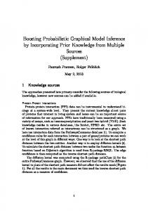
potentials in the graphical model. Moreover, it ensures that every such subset is represented precisely once (and not repeatedly) by an ordered sequence of its variables, cf. [30]. The rationale behind this concept is the following: If the flip of one variable and the flip of another variable not connected to the first one do not reduce the energy then it is pointless to try a simultaneous flip of both variables because the (energy increasing) contributions from both flips would sum up. Furthermore, if the flip of a disconnected set of variables reduces the energy then the same and possibly better reductions can be obtained by flipping connected subsets of this set consecutively, in any order. All disconnected subsets of variables can therefore be excluded from the search if the connected subsets are searched ordered by their size. Finding a unique representative for each connected subset of variables is important. The alternative would be to consider all sequences of pairwise distinct variables in which each variable is connected to at least one of its predecessors and to ignore the fact that many of these sequences represent the same set. Sampling algorithms that select and grow connected subsets in a randomized fashion do exactly this. However, the redundancy is large. As an example, consider a connected subset of six variables of a 2-dimensional grid graph as depicted in Fig. 1a. Although there is only one connected set that contains all six variables, 208 out of the 6! = 720 possible sequences of these variables meet the requirement that each variable is connected to at least one of its predecessors. This 208-fold redundancy hampers the exploration of the search space by means of randomized algorithms; it is avoided in lazy flipping at the cost of storing one unique representative for every connected subgraph in the CS-tree. The second data structure is a tag list that prevents the repeated assessment of unsuccessful flips. The idea is the following: If some variables have been flipped in one iteration (and the current best configuration has been updated accordingly), it suffices to revisit only those sets of variables that are connected to at least one variable that has been flipped. All other sets of variables are excluded from the search because the potentials that depend on these variables are unaffected by the flip and have been assessed in their current state before. The tag list and the connected subgraph tree are essential to the Lazy Flipper and are described in the following sections, 3.1 and 3.2. For a quick overview, the reader can however skip these sections, take for granted that it is possible to efficiently enumerate all connected subgraphs of a graphical model, ordered by their size, and refer directly to the main algorithm (Section 4 and Alg. 1). All non-trivial sub-functions used in the main algorithm are related to tag lists and the CS-tree and are described in detail now. 3.1

Connected Subgraph Tree (CS-tree)

The CS-tree represents subsets of connected variables uniquely. Every node in the CS-tree except the special root node is labeled with the integer index of one variable in the graphical model. The same variable index is assigned to several nodes in the CS-tree unless the graphical model is completely disconnected. The CS-tree is constructed such that every connected subset of variables in the

The Lazy Flipper

5

Fig. 1. All connected subgraphs of a graphical model (a) can be represented uniquely in a connected subgraph tree (CS-tree) (b). Every path from a node in the CS-tree to the root node corresponds to a connected subgraph in the graphical model. While there are 26 = 64 subsets of variables in total in this example, only 40 of these subsets are connected.

graphical model corresponds to precisely one path in the CS-tree from a node to the root node, the node labels along the path indicating precisely the variables in the subset, and vice versa, there exists precisely one connected subset of variables in the graphical model for each path in the CS-tree from a node to the root node. In order to guarantee by construction of the CS-tree that each subset of connected variables is represented precisely once, the variable indices of each subset are put in a special order, namely the lexicographically smallest order in which each variable is connected to at least one of its predecessors. The following definition of these sequences of variable indices is recursive and therefore motivates an algorithm for the construction of the CS-tree for the Lazy Flipper. A small grid model and its complete CS-tree are depicted in Fig. 1. Definition 1 (CSR-Sequence). Given an undirected graph G = (V, E) whose m ∈ N vertices V = {1, . . . , m} are integer indices, every sequence that consists of only one index is called connected subset representing (CSR). Given n ∈ N and a CSR-sequence (v1 , . . . , vn ), a sequence (v1 , . . . , vn , vn+1 ) of n + 1 indices is called a CSR-sequence precisely if the following conditions hold: (i) vn+1 is not among its predecessors, i.e. ∀j ∈ {1, . . . , n} : vj 6= vn+1 . (ii) vn+1 is connected to at least one of its predecessors, i.e. ∃j ∈ {1, . . . , n} : {vj , vn+1 } ∈ E. (iii) vn+1 > v1 . (iv) If n ≥ 2 and vn+1 could have been added at an earlier position j ∈ {2, . . . , n} to the sequence, fulfilling (i)–(iii), all subsequent vertices vj , . . . , vn

6

B. Andres et al.

are smaller than vn+1 , i.e. ∀j ∈ {2, . . . , n} ({vj−1 , vn+1 } ∈ E ⇒ (∀k ∈ {j, . . . , n} : vk < vn+1 )) .

(1)

Based on this definition, three functions are sufficient to recursively build the CS-tree T of a graphical model G, starting from the root node. The function q = growSubset(T, G, p) appends to a node p in the CS-tree the smallest variable index that is not yet among the children of p and fulfills (i)–(iv) for the CSR-sequence of variable indices on the path from p to the root node. It returns the appended node or the empty set if no suitable variable index exists. The function q = firstSubsetOfSize(T, G, n) traverses the CS-tree on the current deepest level n − 1, calling the function growSubset for each leaf until a node can be appended and thus, the first subset of size n has been found. Finally, the function q = nextSubsetOfSameSize(T, G, p) starts from a node p, finds its parent and traverses from there in level order, calling growSubset for each node to find the length-lexicographic successor of the CSR-sequence associated with the node p, i.e. the representative of the next subset of the same size. These functions are used by the Lazy Flipper (Alg. 1) to construct the CS-tree. In contrast, the traversal of already constructed parts of the CS-tree (when revisiting subsets of variables after successful flips) is performed by functions associated with tag lists which are defined the following section. 3.2

Tag Lists

Tag lists are used to tag variables that are affected by flips. A variable is affected by a flip either because it has been flipped itself or because it is connected (via a potential) to a flipped variable. The tag list data structure comprises a Boolean vector in which each entry corresponds to a variable, indicating whether or not this variable is affected by recent flips. As the total number of variables can be large (106 is not exceptional) and possibly only a few variables are affected by flips, a list of all affected variables is maintained in addition to the vector. This list allows the algorithm to untag all tagged variables without re-initializing the entire Boolean vector. The two fundamental operations on a tag list L are tag(L, x) which tags the variable with the index x, and untagAll (L). For the Lazy Flipper, three special functions are used in addition: Given a tag list L, a (possibly incomplete) CS-tree T , the graphical model G, and a node s ∈ T , tagConnectedVariables(L, T, G, s) tags all variables on the path from s to the root node in T , as well as all nodes that are connected (via a potential in G) to at least one of these nodes. The function s = firstTaggedSubset(L, T ) traverses the first level of T and returns the first node s whose variable is tagged (or the empty set if all variables are untagged). Finally, the function t = nextTaggedSubset(L, T, s) traverses T in level order, starting with the successor of s, and returns the first node t for which the path to the root contains at least one tagged variable. These functions, together with those of the CS-tree, are sufficient for the Lazy Flipper, Alg. 1.

The Lazy Flipper

4

7

The Lazy Flipper Algorithm

In the main loop of the Lazy Flipper (lines 2–26 in Alg. 1), the size n of subsets is incremented until the limit nmax is reached (line 24). Inside this main loop, the algorithm falls into two parts, the exploration part (lines 3–11) and the revisiting part (lines 12–23). In the exploration part, flips of previously unseen subsets of n variables are assessed. The current best configuration c is updated in a greedy fashion, i.e. whenever a flip yields a lower energy. At the same time, the CStree is grown, using the functions defined in Section 3.1. In the revisiting part, all subsets of sizes 1 through n that are affected by recent flips are assessed iteratively until no flip of any of these subsets reduces the energy (line 14). The indices of affected variables are stored in the tag lists L1 and L2 (cf. Section 3.2). In practice, the Lazy Flipper can be stopped at any point, e.g. when a time limit is exceeded, and the current best configuration c taken as the output. It eventually reaches configurations for which it is guaranteed that no flip of n or less variables can yield a lower energy because all such flips that could potentially lower the energy have been assessed (line 14). Such configurations are therefore guaranteed to be optimal within a Hamming radius of n: Definition 2 (Hamming-n bound). Given a function E : {0, 1}m → R, a configuration c ∈ {0, 1}m , and n ∈ N, E(c) is called a Hamming-n upper bound on the minimum of E precisely if ∀c0 ∈ {0, 1}m (|c0 − c|1 ≤ n ⇒ E(c) ≤ E(c0 )).

5

Experiments

For a comparative assessment of the Lazy Flipper, four optimization problems of different complexity are considered, two simulated problems and two problems based on real-world data. For the sake of reproducibility, the simulations are described in detail and the models constructed from real data are available from the authors as supplementary material. The first problem is a ferromagnetic Ising model that is widely used in computer vision for foreground vs. background segmentation [6]. Energy functions of this model consist of first and second order potentials that are submodular. The global minimum can therefore be found via a graph cut. We simulate random instances of this model in order to measure how the runtime of lazy flipping depends on the size of the model and the coupling strength, and to compare Lazy Flipper approximations to the global optimum (Section 5.1). The second problem is a problem of finding optimal subgraphs on a grid. Energy functions of this model consist of first and fourth order potentials, of which the latter are not permutation submodular. We simulate difficult instances of this problem that cannot be solved to optimality, even when allowing several days of runtime. In this challenging setting, Lazy Flipper approximations and their convergence are compared to those of BP, TRBP and DD as well as to the lower bounds on local polytope relaxations obtained by DD (Section 5.2).

8

B. Andres et al.

Algorithm 1: Lazy Flipper

1 2 3 4 5 6 7 8 9 10 11 12 13 14 15 16 17 18 19 20 21 22 23 24 25 26

Input: G: graphical model with m ∈ N binary variables, c ∈ {0, 1}m : initial configuration, nmax ∈ N: maximum size of subgraphs to be searched Output: c ∈ {0, 1}m (modified): configuration corresponding to the smallest upper bound found (c is optimal within a Hamming radius of nmax ). n ← 1; CS-Tree T ← {root}; TagList L1 ← ∅, L2 ← ∅; repeat s ← firstSubsetOfSize(T, G, n); if s = ∅ then break; while s 6= ∅ do if energyAfterFlip(G, c, s) < energy(G, c) then c ← flip(c, s); tagConnectedVariables(L1 , T, G, s); end s ← nextSubsetOfSameSize(T, G, s); end repeat s2 ← firstTaggedSubset(L1 , T ); if s2 = ∅ then break; while s2 6= ∅ do if energyAfterFlip(G, c, s2 ) < energy(G, c) then c ← flip(c, s2 ); tagConnectedVariables(L2 , T, G, s2 ); end s2 ← nextTaggedSubset(L1 , T, s2 ); end untagAll(L1 ); swap(L1 , L2 ); end if n = nmax then break; n ← n + 1; end

The third problem is a graphical model for removing excessive boundaries from image over-segmentations that is related to the model proposed in [31]. Energy functions of this model consist of first, third and fourth order potentials. In contrast to the grid graphs of the Ising model and the optimal subgraph model, the corresponding factor graphs are irregular but still planar. The higher-order potentials are not permutation submodular but the global optimum can be found by means of MILP in approximately 10 seconds per model using one of the fastest commercial solvers (IBM ILOG CPLEX, version 12.1). Since CPLEX is closedsource software, the algorithm is not known in detail and we use it as a black box. The general method used by CPLEX for MILP is a branch-and-bound algorithm [32,33]. 100 instances of this model obtained from the 100 natural test images of the Berkeley Segmentation Database (BSD) [34] are used to compare the Lazy Flipper to algorithms based on message passing and linear programming in a real-world setting where the global optimum is accessible (Section 5.3).

The Lazy Flipper

9

The fourth problem is identical to the third, except that instances are obtained from 3-dimensional volume images of neural tissue acquired by means of Serial Block Face Scanning Electron Microscopy (SBFSEM) [35]. Unlike in the 2-dimensional case, the factor graphs are no longer planar. Whether exact optimization by means of MILP is practical depends on the size of the model. In practice, SBFSEM datasets consist of more than 20003 voxels. To be able to compare approximations to the global optimum, we consider 16 models obtained from 16 SBFSEM volume sub-images of only 1503 voxels for which the global optimum can be found by means of MILP within a few minutes (Section 5.4). 5.1

Ferromagnetic Ising model

The ferromagnetic Ising model consists of m ∈ N binary variables x1 , . . . , xm ∈ {0, 1} that are associated with points on a 2-dimensional square grid and connected via second order potentials Ejk (xj , xk ) = 1 − δxj ,xk (δ: Kronecker delta) to their nearest neighbors. First order potentials Ej (xj ) relate the variables to observed evidence in underlying data. The total energy of this model is the following sum in which α ∈ R+ 0 is a weight on the second order potentials, and j ∼ k indicates that the variables xj and xk are adjacent on the grid: m

∀x ∈ {0, 1}

:

E(x) =

m X j=1

Ej (xj ) + α

m X m X

Ejk (xj , xk ) .

(2)

j=1 k=j+1 k∼j

For each α ∈ {0.1, 0.3, 0.5, 0.7, 0.9}, an ensemble of ten simulated Ising models of 50 · 50 = 2500 variables is considered. The first order potentials Ej are initialized randomly by drawing Ej (0) uniformly from the interval [0, 1] and setting Ej (1) := 1 − Ej (0). The exact global minimum of the total energy is found via a graph cut. For each model, the Lazy Flipper is initialized with a configuration that minimizes the sum of the first order potentials. Upper bounds on the minimum energy found by means of lazy flipping converge towards the global optimum as depicted in Fig. 2. Color scales and gray scales in this figure respectively indicate the maximum size and the total number of distinct subsets that have been searched, averaged over all models in the ensemble. It can be seen from this figure that upper bounds on the minimum energy are tightened significantly by searching larger subsets of variables, independent of the coupling strength α. It takes the Lazy Flipper less than 100 seconds (on a single CPU of an Intel Quad Xeon E7220 at 2.93GHz) to exhaustively search all connected subsets of 6 variables. The amount of RAM required for the CS-tree (in bytes) is 24 times as high as the number of subsets (approximately 50 MB in this case) because each subset is stored in the CS-tree as a node consisting of three 64-bit integers: a variable index, the index of the parent node and the index of the level order successor (Section 3.1)1 . 1

The size of the CS-tree becomes limiting for very large problems. However, for regular graphs, implicit representations can be envisaged that overcome this limitation.

10

B. Andres et al.

For nmax ∈ {1, 6}, configurations corresponding to the upper bounds on the minimum energy are depicted in Fig. 3. It can be seen from this figure that all connected subsets of falsely set variables are larger than nmax . For a fixed maximum subgraph size nmax , the runtime of lazy flipping scales approximately linearly with the number of variables in the Ising model (cf. Fig.4). 5.2

Optimal Subgraph Model

The optimal subgraph model consists of m ∈ N binary variables x1 , . . . , xm ∈ {0, 1} that are associated with the edges of a 2-dimensional grid graph. A subgraph is defined by those edges whose associated variables attain the value 1. Energy functions of this model consist of first order potentials, one for each edge, and fourth order potentials, one for each node v ∈ V in which four edges (j, k, l, m) = N (v) meet: ∀x ∈ {0, 1}m :

E(x) =

m X j=1

Ej (xj ) +

X

Ejklm (xj , xk , xl , xm ) .

(3)

(j,k,l,m)∈N (V )

All fourth order potentials are equal, penalizing dead ends and branches of paths in the selected subgraph:   0.0 if s = 0      100.0 if s=1  Ejklm (xj , xk , xl , xm ) = 0.6 if s = 2 with s = xj + xk + xl + xm . (4)    1.2 if s=3    2.4 if s = 4 An ensemble of 16 such models is constructed by drawing the unary potentials at random, exactly as for the Ising models. Each model has 19800 variables, the same number of first order potentials, and 9801 fourth order potentials. Approximate optimal subgraphs are found by Min-Sum Belief Propagation (BP) with parallel message passing [9,14] and message damping [36], by Tree-reweighted Belief Propagation (TRBP) [4], by Dual Decomposition (DD) [16,17] and by lazy flipping (LF). DD affords also lower bounds on the minimum energy. Details on the parameters of the algorithms and the decomposition of the models are given in Appendix A. Bounds on the minimum energy converge with increasing runtime, as depicted in Fig. 5. It can be seen from this figure that Lazy Flipper approximations converge fast, reaching a smaller energy after 3 seconds than the other approximations after 10000 seconds. Subgraphs of up to 7 variables are searched, using approximately 2.2 GB of RAM for the CS-tree. A gap remains between the energies of all approximations and the lower bound on the minimum energy obtained by DD. Thus, there is no guarantee that any of the problems has been solved to optimality. However, the gaps are upper bounds on the deviation from the global optimum. They are compared at t = 10000 s in Fig. 5. For any model in the

The Lazy Flipper α=0.1

4

10

8.0 2⋅106

3

10

2

2

10 ELF − Eopt

10 ELF − Eopt

7.1 2⋅106

3

10

1

10

0

1

10

0

10

10

−1

−1

10

10

min/max median

−2

10

α=0.3

4

10

−3

10

−2

10

min/max median

−2

−1

0

10

10

1

10

10

2

10

−3

10

−2

10

−1

7.1 2⋅106

3

10

10

2

2

10 ELF − Eopt

10 ELF − Eopt

10

10

7.0 2⋅106

3

1

10

0

1

10

0

10

10

−1

−1

10

10

min/max median

−2 −3

10

−2

10

min/max median

−2

−1

0

10

10

1

10

10

2

10

−3

10

−2

10

−1

0

10

t [s]

1

10

2

10

10

t [s]

α=0.9

4

10

7.4 2⋅106

t=100s

3

10

0.08 (ELF − Eopt) / Eopt

2

10 ELF − Eopt

2

10

α=0.7

4

10

1

10

0

10

0.06 0.04 0.02

−1

10

min/max median

−2

10

1

10 t [s]

α=0.5

4

0

10

t [s]

10

11

−3

10

−2

10

−1

0

10

10 t [s]

1

10

2

10

0 0.1

0.3

0.5 α

0.7

0.9

Fig. 2. Upper bounds on the minimum energy of a graphical model can be found by flipping subsets of variables. The deviation of these upper bounds from the minimum energy is shown above for ensembles of ten random Ising models (Section 5.1). Compared to optimization by ICM where only one variable is flipped at a time, the Lazy Flipper finds significantly tighter bounds by flipping also larger subsets. The deviations increase with the coupling strength α. Color scales and gray scales indicate the size and the total number of searched subsets.

12

B. Andres et al. nmax

α = 0.1

α = 0.3

α = 0.5

α = 0.7

α = 0.9

1

6

∞

Fig. 3. The configurations found by the Lazy Flipper converge to a global optimum as the search depth nmax increases. For Ising models with different coupling strengths α (columns), deviations from the global optimum (nmax = ∞) are depicted in blue (false 0) and orange (false 1), for nmax ∈ {1, 6}. As the Lazy Flipper is greedy, these approximate solutions highly depend on the initialization and on the order in which subsets are visited. 350 Nmodels = 10, nmax = 6 300

Runtime [s]

250 200 150 100 50 0 0

2000

4000 6000 8000 Number of variables

10000

12000

Fig. 4. For a fixed maximum subgraph size (nmax = 6), the runtime of lazy flipping scales only slightly more than linearly with the number of variables in the Ising model. It is measured for coupling strengths α = 0.25 (upper curve) and α = 0.75 (lower curve). Error bars indicate the standard deviation over 10 random models, and lines are fitted by least squares. Lazy flipping takes longer (0.0259 seconds per variable) for α = 0.25 than for α = 0.75 (0.0218 s/var) because more flips are successful and thus initiate revisiting.

The Lazy Flipper

13

ensemble, the energy of the Lazy Flipper approximation is less than 4% away from the global optimum, a substantial improvement over the other algorithms for this particular model. 5.3

Pruning of 2D Over-Segmentations

The graphical model for removing excessive boundaries from image over-segmentations contains one binary variable for each boundary between segments, indicating whether this boundary is to be removed (0) or preserved (1). First order potentials relate these variables to the image content, and non-submodular third and fourth order potentials connect adjacent boundaries, supporting the closedness and smooth continuation of preserved boundaries. The energy function is a sum of these potentials: ∀x ∈ {0, 1}m E(x) =

m X j=1

Ej (xj ) +

X

Ejkl (xj , xk , xl ) +

(j,k,l)∈J

X

Ejklp (xj , xk , xl , xp ) .

(5)

(j,k,l,p)∈K

We consider an ensemble of 100 such models obtained from the 100 BSD test images [34]. On average, a model has 8845 ± 670 binary variables, the same number of unary potentials, 5715 ± 430 third order potentials and 98 ± 18 fourth order potentials. Each variable is connected via potentials to at most six other variables, a sparse structure that is favorable for the Lazy Flipper. BP, TRBP, DD and the Lazy Flipper solve these problems approximately, thus providing upper bounds on the minimum energy. The differences between these bounds and the global optimum found by means of MILP are depicted in Fig. 6. It can be seen from this figure that, after 200 seconds, Lazy Flipper approximations provide a tighter upper bound on the global minimum in the median than those of the other three algorithms. BP and DD have a better peak performance, solving one problem to optimality. The Lazy Flipper reaches a search depth of 9 after around 1000 seconds for these sparse graphical models using roughly 720 MB of RAM for the CS-tree. At t = 5000 s and on average over all models, its approximations deviate by only 2.6% from the global optimum. 5.4

Pruning of 3D Over-Segmentations

The model described in the previous section is now applied in 3D to remove excessive boundaries from the over-segmentation of a volume image. In an ensemble of 16 such models obtained from 16 SBFSEM volume images, models have on average 16748 ± 1521 binary variables (and first order potentials), 26379 ± 2502 potentials of order 3, and 5081 ± 482 potentials of order 4. For BP, TRBP, DD and Lazy Flipper approximations, deviations from the global optimum are shown in Fig. 7. It can be seen from this figure that BP performs exceptionally well on these problems, providing approximations whose energies deviate by only 0.4% on average from the global optimum. One reason is that most variables influence many (up to 60) potential functions, and BP

14

B. Andres et al. 5

5

10

EBP

ETRBP

10

4

4

10

10 min/max median

Belief Propagation −2

10

−1

10

0

10

1

10 t [s]

2

10

3

10

min/max median

TRBP 4

−2

10

10

5

−1

10

0

10

1

10 t [s]

2

10

3

10

4

10

5

10

7.0 9⋅107

ELF

EDD

10

4

4

10

10 min/max median

Dual Decomposition −2

10

−1

10

0

10

1

10 t [s]

2

10

3

10

min/max median

Lazy Flipper 4

10

−2

10

−1

10

0

10

1

10 t [s]

2

10

3

10

4

10

t = 10000s

(E − EDD−) / EDD−

1 0.8 0.6 0.4 0.2

63.1%

84.3%

86.6%

3.2%

BP

TRBP

DD

LF

0

Fig. 5. Approximate solutions to the optimal subgraph problem (Section 5.2) are found by BP, TRBP, DD and the Lazy Flipper (LF). Depicted are the median, minimum and maximum (over 16 models) of the corresponding energies. DD affords also lower bounds on the minimum energy. The mean search depth of LF ranges from 1 (yellow) to 7 (red). At t = 104 s, the energies of LF approximations come close to the lower bounds obtained by DD and thus, to the global optimum.

The Lazy Flipper

4

4

10

10

3

3

10 ETRBP − Eopt

EBP − Eopt

10

2

10

1

10

0

2

10

1

10

0

10

10 Belief Propagation

−1

−2

10

−1

10

0

10

1

10 t [s]

2

10

10

3

10

4

−1

10

0

10

1

10 t [s]

2

10

3

10

4

10

3

9.0 7 3⋅10

3

10

10

2

ELF − Eopt

EDD − Eopt

−2

10

10

10

1

10

0

2

10

1

10

0

10

10 Dual Decomposition

Lazy Flipper

−1

10

min/max 0.25/0.75−quantile median

TRBP

−1

10

15

−1

−2

10

−1

10

0

10

1

10 t [s]

2

10

0.5

3

10

10

−2

10

−1

10

0

10

1

10 t [s]

2

10

3

10

t = 5000s

(E − Eopt) / Eopt

0.4 0.3

13.2% 18.9% 14.7%

2.6%

0.2 0.1 0 BP

TRBP

DD

LF

Fig. 6. Approximate solutions to the problem of removing excessive boundaries from over-segmentations of natural images. The search depth of the Lazy Flipper, averaged over all models in the ensemble, ranges from 1 (orange) to 9 (red). At t = 5000 s, 3 · 107 subsets are stored in the CS-tree.

16

B. Andres et al.

can propagate local evidence from all these potentials. Variables are connected via these potentials to as many as 100 neighboring variables which hampers the exploration of the search space by the Lazy Flipper that reaches only of search depth of 5 after 10000 seconds, using 4.8 GB of RAM for the CS-tree, yielding worse approximations than BP, TRBP and DD for these models. In practical applications where volume images and the according models are several hundred times larger and can no longer be optimized exactly, it matters whether one can further improve upon the BP approximations. Dashed lines in the first plot in Fig. 7 show the result obtained when initializing the Lazy Flipper with the BP approximation at t = 100s. This reduces the deviation from the global optimum at t = 50000 s from 0.4% on average over all models to 0.1%.

6

Conclusion

The optimum of a function of binary variables that decomposes according to a graphical model can be found by an exhaustive search over only the connected subgraphs of the model. We implemented this search, using a CS-tree to efficiently and uniquely enumerate the subgraphs. The C++ source code is available from http://hci.iwr.uni-heidelberg.de/software.php. Our algorithm is guaranteed to converge to a global minimum when searching through all subgraphs which is typically intractable. With limited runtime, approximations can be found by restricting the search to subgraphs of a given maximum size. Simulated and real-world problems exist for which these approximations compare favorably to those obtained by message passing and sub-gradient descent. For large scale problems, the applicability of the Lazy Flipper is limited by the memory required for the CS-tree. However, for regular graphs, this limit can be overcome by an implicit representation of the CS-tree that is subject of future research.

Acknowledgments Acknowledgement pending approval by the acknowledged individuals.

A

Parameters and Model Decomposition

In all experiments, the damping parameters for BP and TRBP are chosen optimally from the set {0, 0.1, 0.2, . . . , 0.9}. The step size of the sub-gradient descent is chosen according to 1 (6) τt = α 1 + βt where β = 0.01 and α is chosen optimally from {0.01, 0.025, 0.05, 0.1, 0.25, 0.5}. The sequence of step sizes, in particular the function (6) and β could be tuned

The Lazy Flipper 4

4

10

10

3

3

10 ETRBP − Eopt

EBP − Eopt

10

2

10

1

10

0

BP (+ Lazy Flipper) −2

10

−1

10

0

10

1

10 10 t [s]

3

10

10

4

10

−2

10

4

min/max 0.25/0.75−quantile median

TRBP

−1

2

−1

10

0

10

1

2

10 10 t [s]

3

10

4

10

4

10

10

3

5.0 8 2⋅10

3

10

10

2

ELF − Eopt

EDD − Eopt

1

10

10

−1

10

1

10

0

2

10

1

10

0

10

10 Dual Decomposition

−1

10

2

10

0

10

10

17

−2

10

−1

10

0

10

1

Lazy Flipper

−1

2

10 10 t [s]

0.3

3

10

4

10

10

−2

10

−1

10

0

10

1

2

10 10 t [s]

3

10

4

10

t = 50000s

(E − Eopt) / Eopt

0.25 0.4%

0.1%

4.8%

9.6% 13.2%

0.2 0.15 0.1 0.05 0 BP

BP+LF TRBP

DD

LF

Fig. 7. Approximate solutions to the problem of removing excessive boundaries from over-segmentations of 3-dimensional volume images. The search depth of the Lazy Flipper, averaged over all models in the ensemble, ranges from 1 (yellow) to 5 (purple). After 50000 s, 2·108 subsets are stored in the CS-tree. Dashed lines in the first plot show the result obtained when initializing the Lazy Flipper with the BP approximation at t = 100s. This reduces the deviation from the global optimum at t = 50000 s from 0.4% on average over all models to 0.1%.

18

B. Andres et al.

further. Moreover, [16] consider the primal-dual gap and [17] smooth the subgradient over iterations in order to suppress oscillations. These measures can have substantial impact on the convergence. The upper bounds obtained by BP, TRBP and DD do not decrease monotonously. After each iteration of these algorithms, we therefore consider the elapsed runtime and the current best bound, i.e. the best bound of the current and all preceding iterations. All five algorithms are implemented in C++, using the same optimized data structures for the graphical model and a visitor design pattern that allows us to measure runtime without significantly affecting performance. The same decomposition of each graphical model into tree models is used for TRBP and DD. Tree models are constructed in a greedy fashion, each comprising as many potential functions as possible. The procedure is generally applicable to irregular models with higher-order potentials: Initially, all potentials of the graphical model are put on a white list that contains those potentials that have not been added to any tree model. A black list of already added potentials and a gray list of recently added potentials are initially empty. As long as there are potentials on the white list, new tree models are constructed. For each newly constructed tree model, the procedure iterates over the white list, adding potentials to the tree model if they do not introduce loops. Added potentials are moved from the white list to the gray list. After all potentials from the white list have been processed, potentials from the black list that do not introduce loops are added to the tree model. The gray list is then appended to the black list and cleared. The procedure finishes when the white list is empty. As recently shown in [17], decompositions into cyclic subproblems can lead to significantly tighter relaxations and better integer solutions.

References 1. Cowell, R.G., Dawid, A.P., Lauritzen, S.L., Spiegelhalter, D.J.: Probabilistic Networks and Expert Systems: Exact Computational Methods for Bayesian Networks. Springer (2007) 2. Koller, D., Friedman, N.: Probabilistic Graphical Models. MIT Press (2009) 3. Lauritzen, S.L.: Graphical Models. Statistical Science. Oxford (1996) 4. Wainwright, M.J., Jordan, M.I.: Graphical Models, Exponential Families, and Variational Inference. Now Publishers Inc., Hanover, MA, USA (2008) 5. Besag, J.: On the statisical analysis of dirty pictures. Journal of the Royal Statistical Society B 48 (1986) 259–302 6. Boykov, Y., Veksler, O., Zabih, R.: Fast approximate energy minimization via graph cuts. Transactions on Pattern Analysis and Machine Intelligence 23 (2001) 1222–1239 7. Geman, S., Geman, D.: Stochastic relaxation, gibbs distribution and the bayesian restoration of images. Transactions on Pattern Analysis and Machine Intelligence 6 (1984) 721–741 8. McEliece, R., MacKay, D., Cheng, J.F.: Turbo decoding as an instance of pearl’s belief propagation algorithm. IEEE Journal on Selected Areas in Communications 16 (1998) 140–152

The Lazy Flipper

19

9. Pearl, J.: Probabilistic reasoning in intelligent systems: networks of plausible inference. Morgan Kaufmann, San Francisco, CA, USA (1988) 10. Kolmogorov, V., Zabin, R.: What energy functions can be minimized via graph cuts? Transactions on Pattern Analysis and Machine Intelligence 26 (2004) 147– 159 11. Schlesinger, D.: Exact solution of permuted submodular MinSum problems. In: Proceedings of the 6th EMMCVPR. (2007) 12. Schrijver, A.: Theory of linear and integer programming. John Wiley & Sons, Inc., New York, NY, USA (1986) 13. Schrijver, A.: Combinatorial Optimization: Polyhedra and Efficiency. Springer (2003) 14. Kschischang, F.R., Frey, B.J., Loeliger, H.: Factor graphs and the sum-product algorithm. Transactions on Information Theory 47 (2001) 498–519 15. Wainwright, M.J., Jaakkola, T., Willsky, A.S.: MAP estimation via agreement on trees: message-passing and linear programming. IEEE Transactions on Information Theory 51 (2005) 3697–3717 16. Komodakis, N., Paragios, N., Tziritas, G.: MRF energy minimization and beyond via dual decomposition. Transactions on Pattern Analysis and Machine Intelligence 99 (2010) 17. Kappes, J.H., Schmidt, S., Schnoerr, C.: MRF inference by k-fan decomposition and tight Lagrangian relaxation. In: European Conference on Computer Vision 2010. (2010) 18. Frey, B.J., Jojic, N.: A comparison of algorithms for inference and learning in probabilistic graphical models. Transactions on Pattern Analysis and Machine Intelligence 27 (2005) 1392–1416 19. Jung, K., Kohli, P., Shah, D.: Local rules for global MAP: When do they work? In Bengio, Y., Schuurmans, D., Lafferty, J., Williams, C.K.I., Culotta, A., eds.: Advances in Neural Information Processing Systems 22. (2009) 871–879 20. Swendsen, R.H., Wang, J.S.: Nonuniversal critical dynamics in monte carlo simulations. Physical Review Letters 58 (1987) 86–88 21. Wolff, U.: Collective monte carlo updating for spin systems. Physical Review Letters 62 (1989) 361–364 22. Barbu, A., Zhu, S.C.: Graph partition by Swendsen-Wang cuts. In: Proceedings of the Ninth IEEE International Conference on Computer Vision, Washington, DC, USA, IEEE Computer Society (2003) 320 23. Minka, T.P.: Expectation propagation for approximate Bayesian inference. In: Proceedings of the 17th Conference on Uncertainty in Artificial Intelligence. (2001) 362–369 24. Globerson, A., Jaakkola, T.: Fixing max-product: Convergent message passing algorithms for MAP LP-relaxations. In: Advances in Neural Information Processing Systems, Cambridge, MA, USA, MIT Press (2007) 553–560 25. Werner, T.: A linear programming approach to max-sum problem: A review. Transactions on Pattern Analysis and Machine Intelligence 29 (2007) 1165–1179 26. Kohli, P., Shekhovtsov, A., Rother, C., Kolmogorov, V., Torr, P.: On partial optimality in multi-label MRFs. In: Proceedings of the 25th International Conference on Machine Learning. (2008) 27. Kumar, M.P., Kolmogorov, V., Torr, P.H.S.: An analysis of convex relaxations for MAP estimation of discrete MRFs. Journal of Machine Learning Research 10 (2009) 71–106

20

B. Andres et al.

28. Kolmogorov, V.: Convergent tree-reweighted message passing for energy minimization. Transactions on Pattern Analysis and Machine Intelligence 28 (2006) 1568–1583 29. Weiss, Y., Freeman, W.: On the optimality of solutions of the max-product beliefpropagation algorithm in arbitrary graphs. IEEE Transactions on Information Theory 47 (2001) 736 –744 30. Moerkotte, G., Neumann, T.: Analysis of two existing and one new dynamic programming algorithm for the generation of optimal bushy join trees without cross products. In: Proceedings of the 32nd International Conference on Very Large Data Bases. (2006) 31. Zhang, L., Ji, Q.: Image segmentation with a unified graphical model. Transactions on Pattern Analysis and Machine Intelligence 32 (2010) 1406–1425 32. Dakin, R.J.: A tree-search algorithm for mixed integer programming problems. Computer Journal 8 (1965) 250–255 33. Land, A.H., Doig, A.G.: An automatic method of solving discrete programming problems. Econometrica 28 (1960) 497–520 34. Martin, D., Fowlkes, C., Tal, D., Malik, J.: A database of human segmented natural images and its application to evaluating segmentation algorithms and measuring ecological statistics. In: Proceedings of the 8th International Conference on Computer Vision (ICCV). Volume 2. (2001) 416–423 35. Denk, W., Horstmann, H.: Serial block-face scanning electron microscopy to reconstruct three-dimensional tissue nanostructure. PLoS Biology 2 (2004) e329 36. Murphy, K.P., Weiss, Y., Jordan, M.I.: Loopy belief propagation for approximate inference: An empirical study. In: Proceedings of Uncertainty in AI. (1999) 467–475