THE LINEARIZED SPLIT BREGMAN ITERATIVE ALGORITHM AND

1

THE LINEARIZED SPLIT BREGMAN ITERATIVE ALGORITHM AND ITS CONVERGENCE ANALYSIS FOR ROBUST TOMOGRAPHIC IMAGE RECONSTRUCTION † CHONG CHEN

‡ AND

GUOLIANG XU

§

Abstract. The split Bregman iteration method has been successfully applied to solve a variety of specially ℓ1 -regularized problems, such as image denoising, image segmentation, magnetic resonance imaging reconstruction, and so forth. There exists, however, a large-scale and unstructured linear system demanding to be resolved in each iteration for the robust image reconstruction problem in sparse-view X-ray computed tomography. Motivated by this, we propose a new linearized split Bregman iterative algorithm, which is constructed by means of the thoughts of split and linearized Bregman methods. Remarkably, our method can be generalized to efficiently resolve the robust compressed sensing problem, as well as the total variation-ℓ1 and ℓ1 -ℓ1 minimization problems. We also give a rigorous proof for the convergence of the proposed method under appropriate condition, in which the convergence does not depend on the selection of the regularization parameter. Along with the proof idea, we further prove the convergence of the gradient-descent-based split Bregman iteration, yet which relies on the value of the regularization parameter. Hence, our proposed method is more flexible and stable than the split Bregman method. Experimental results demonstrate that our algorithm has better performance in terms of reconstruction quality, effectiveness and robustness, compared with some other frequently used methods for the robust image reconstruction in sparseview X-ray computed tomography. Key words. Linearized split Bregman iteration, split Bregman iteration, linearized Bregman iteration, ℓ1 regularization, robust image reconstruction, sparse-view X-ray computed tomography. AMS subject classifications. 65K05, 65R32, 92C55

1. Introduction In modern commercial X-ray computed tomography (CT) imaging, the projections are generally detected at a large number (more than 300) of views from the patient for high-quality image reconstruction by currently analytic-based algorithms, for instance, filtered back-projection (FBP) method [17, 39, 37, 24]. However, data collection from so large number of views, meaning high doses of radiation, likely result in radiation-induced cancer with high probability [16]. It is of practical interest and meaningful, therefore, to develop imaging techniques that are capable of producing high-quality reconstructions from sparse-view projection data. In recent years, the optimization- or variation-based image reconstruction models and the algorithms of interest have been investigated heavily owing to their ability to allow reducing scanning views while maintaining or improving reconstructed image quality for robust image reconstruction problem arising in sparse-view CT [13, 35, 31, 10, 24, 34]. The rationale behind these studies is considerably similar to compressed sensing (CS), though the non-random projection matrix of CT scanner may well be not satisfying ∗ The

work of C. Chen was supported in part by National Natural Science Foundation of China (NSFC) under the grant 11301520. The work of G. Xu was supported in part by NSFC key project under the grant 10990013, NSFC under the grants 11101401, 81173663 and NSFC Funds for Creative Research Groups of China under the grant 11021101. † Received date / Revised version date ‡ State Key Laboratory of Scientific and Engineering Computing, Institute of Computational Mathematics and Scientific/Engineering Computing, Academy of Mathematics and Systems Science, Chinese Academy of Sciences, P.O. Box 2719, Beijing 100190, P.R. China, ([email protected]). § State Key Laboratory of Scientific and Engineering Computing, Institute of Computational Mathematics and Scientific/Engineering Computing, Academy of Mathematics and Systems Science, Chinese Academy of Sciences, P.O. Box 2719, Beijing 100190, P.R. China, ([email protected]). 1

2

LINEARIZED SPLIT BREGMAN ITERATIVE ALGORITHM

the restricted isometry property which is required to accurately restore the original signal via the CS theory [14, 4, 5, 3]. In a general formulation of the CT reconstruction problem, the reconstructed image can be denoted as a weighted sum of the shifted basis functions (usually pixel/voxel basis) [12]. The discrete projection data g ∈ RM is related to these weights via a linear equations as follows Pf ≈g

or

g = P f + ε,

(1.1)

where f ∈ RN is represented as the vector of weights, P ∈ RM ×N is the projection matrix for modeling the X-ray transform and ε is the interference component. Due to the data inconsistencies, introduced by the approximation to the coefficient elements and the interference of the noise, error, and some other factors, (1.1) is often used to simulate the CT-imaging process. In addition, we should note that both f and P depend on the selection of the shifted basis functions to expand the image function and the way to discrete the the X-ray transform. In this article, we choose the pixel/voxel functions as the basis, and use the intersection length of the X ray with the image pixel/voxel as the elements of the projection matrix. Considering the image reconstruction in the sparse-view X-ray CT, we definitely suffer from the severely under-sampling for M < N , in many cases, M ≪ N . In such a case, the study on the optimization- or variation-based image reconstruction models and the induced algorithms has begun to be in fashion. It is well-known that the iterative tomographic reconstruction algorithms, for solving the optimizing or variational models, are able to yield high-quality images from the limited data. That is because they can take into account the prior knowledge about the solution to regularize the under-determined problem. Often in medical and other applications, the tomographic images are relatively piecewise-constant over the extended volumes, for instance within an organ. Rapid variation in the image may only occur at boundaries of internal structures. Thus an image itself might not be sparse, yet the image formed by taking the magnitude of its gradient can be approximately sparse [33, 35, 31]. Hence, the total variation (TV) based optimizing or variational image reconstruction models were introduced (See [12, 9, 13, 35, 42, 10] and the references therein). In this paper, we mainly concern the following model for such a problem min J(f ), f

subject to ∥P f − g∥2 ≤ σ,

where J(f ) = ∥∇f ∥1 denotes the TV semi-norm. The above constrained optimization is equivalent to the following unconstrained optimization problem λ min J(f ) + ∥P f − g∥22 . f 2 A brief proof on their equivalency can be found in Section 3. To solve above reconstruction models efficiently, a variety of algorithms have been proposed, such as gradient descend method [33, 29], improved gradient descend method [38], adaptivesteepest-descent projection onto convex sets method [35, 36], split Bregman iteration [22], gradient-flow-based finite element methods [42, 10, 11], etc. Although the split Bregman iteration is extremely efficient, it just can fast solve the problems that have certain special structure in matrix P , for instance, TV denoising and segmentation (P is an identity matrix), magnetic resonance imaging reconstruction (P comprises a subset of the rows of the Fourier transform matrix), and

3

C. CHEN AND G. XU

so forth [22, 21]. For CT image reconstruction, the projection matrix P has not been figured out the particular structure so as to fast deal with the inversion matrix of P T P in each iteration. The details about this problem is given in Section 2. In this work, we present a novel algorithm, called linearized split Bregman (LSB) iteration, that can be well suited to efficiently solving the sparse-view CT image reconstruction problem. Notably, the idea we provide can be generalized to solve a variety of optimization or variation models, which are considerably significant in practice and are hard to resolve by the existing methods. For instance, the robust CS problem λ min ∥f ∥1 + ∥P f − g∥22 , f 2 where P is a sensing matrix [6]. Recently, there exist many efficiently algorithms to solve this model, for instance, fixed-point continuation [23], alternative direction method (ADM) (See [19, 20, 44] and the references therein). Furthermore, our proposed method is able to solve the models that use the ℓ1 -norm as the measure of fidelity [27, 8, 18, 41], such as the TV-ℓ1 minimization problem λ min ∥∇f ∥1 + ∥P f − g∥1 , f 2 and the ℓ1 -ℓ1 minimization problem λ min ∥f ∥1 + ∥P f − g∥1 . f 2 We also give a rigorous proof on the convergence of the proposed method under appropriate condition for each extension, in which the convergence does not depend on the selection of the regularization parameter. As a previous work, Cai et al. proved the convergence of the unconstrained/constrained split Bregman iterations in [2], while their proofs are merely concerning the iterative schemes based on solving each subproblem exactly. Admittedly, it is almost impossible to precisely or directly resolve the general large-scale linear system in related subproblem. It means that the practically iterative algorithms of interest must be applied, for instance, the gradient descent method, conjugate gradient method, Gauss-Siedel method, etc. Along with our proof idea, we further prove the convergence of the gradient-decent-based split Bregman (GDSB) method. The rest of the paper is organized as follows. In Section 2, we first briefly review the classical Bregman methods and point out the existing difficulties of them in solving the robust CT image reconstruction problem. We then propose an LSB iterative algorithm and generalize it to solve a variety of ℓ1 -optimization problems in Section 3. In Section 4, we give the proof for the convergence of the proposed method, and further analyze the convergence of the GDSB iteration. In Section 5, we apply our algorithm to the robust image reconstruction in sparse-view X-ray CT imaging and make several numerical comparisons with some other methods. Finally, we conclude this paper in Section 6. 2. Classical Bregman iteration algorithms In this section, we first consider the general optimization problem of a convex function on the n-dimensional (nD) Euclidean space Rn . Let J : Rn → R be a convex function. A vector p ∈ Rn is called a subgradient of J at a point v ∈ Rn if J(u) − J(v) − ⟨p,u − v⟩ ≥ 0,

∀u ∈ Rn .

(2.1)

4


The subdifferential ∂J(v) is the set of all subgradients of J at v [32]. The Bregman distance associated with J at v is defined as DJq (u,v) = J(u) − J(v) − ⟨q,u − v⟩,

(2.2)

where p is a subgradient of J at v, namely, p ∈ ∂J(v). Obviously, DJq (u,v) ≥ 0, and DJq (u,v) ≥ DJq (w,v) for any w ∈ Rn on the line segment between u and v. Note that DJq (u,v) ̸= DJq (v,u) in general, namely, the symmetry is not met so that DJq (u,v) is not a distance in the usual sense [1, 28]. 2.1. Bregman iteration algorithm Considering the following optimization problem min J(f ), f

subject to P f = g,

(2.3)

where if J(f ) = ∥∇f ∥1 , this model is often applied to image deblurring and tomographic image reconstruction; if J(f ) = ∥f ∥1 , that is frequently solved in basis pursuit problem or compressed sensing [28, 40, 22, 46]. Notice that the observational data g are not corrupted by noise in (2.3). The Bregman iteration was first applied in image processing in [28], and then used to solve the ℓ1 -minimization problem with application to compressed sensing, which is equivalent to the well-known augmented Lagrangian method [46, 20]. We summarize the Bregman iteration for solving the minimization problem (2.3) as follows k λ f k+1 = argmin DJq (f,f k ) + ∥P f − g∥22 , f 2

(2.4)

q k+1 = q k − λP T (P f k+1 − g).

(2.5)

As shown in [46, 25], the above seemingly complicated Bregman iteration is equivalent to the following simplified iterative scheme λ f k+1 = argmin J(f ) + ∥P f − bk ∥22 , f 2

(2.6)

bk+1 = bk + g − P f k+1 .

(2.7)

The main advantages of the Bregman iteration include that the convergent rate is very fast when it is employed to certain types of optimization problems and the value of the penalty factor λ is not required to tend to infinity during computation. 2.2. Split Bregman iteration algorithm When J(f ) = ∥∇f ∥1 , the unconstrained optimization subproblem (2.6) has no closed-form solution and is difficult to solve since the cost function contains the ℓ1 and ℓ2 portions simultaneously. To overcome this problem, Goldstein and Osher presented an algorithm called split Bregman method to solve this optimization problem effectively [22]. The key idea of their algorithm is that they decoupled the ℓ1 and ℓ2 terms of the cost function in (2.6). The splitting thought is also proposed in [40] with application to ℓ1 -regularized deconvolution. Hence, they considered the following minimization problem λ min ∥d∥1 + ∥P f − g∥22 , f,d 2

subject to d = ∇f.

(2.8)

C. CHEN AND G. XU

5

In what follows the split Bregman iteration algorithm to solve above problem is presented. λ µ (f k+1 ,dk+1 ) = argmin ∥d∥1 + ∥P f − g∥22 + ∥d − ∇f − sk ∥22 , f,d 2 2 sk+1 = sk + ∇f k+1 − dk+1 .

(2.9) (2.10)

Note that the subproblem (2.9) should be precisely resolved. Hence a lot of inner iterations are needed. The concrete implementation, with the inner iteration number fixed to be 1, is given as the following Algorithm 2.1. Algorithm 2.1. Split Bregman Iteration Algorithm Step 1. Given initial points f 0 = 0, d0 = 0, s0 = 0, 0 < ϵ ≪ 1 and an integer K > 0. Set k := 0. Step 2. Update d: µ dk+1 = argmin ∥d∥1 + ∥d − ∇f k − sk ∥22 . d 2

(2.11)

λ µ f k+1 = argmin ∥P f − g∥22 + ∥dk+1 − ∇f − sk ∥22 . f 2 2

(2.12)

Step 3. Update f :

Compute rk = ∥f k+1 − f k ∥2 . If rk < ϵ or k + 1 > K, stop the iteration, otherwise go to the next step. Step 4. Update s: sk+1 = sk + ∇f k+1 − dk+1 . Step 5. Set k := k + 1, return to Step 2. Notably, the Step 2 and Step 3 should be precisely resolved to guarantee the convergence of the algorithm (See [2]). Fortunately, one can explicitly figure out the minimum dk+1 in Step 2 by using the generalized shrinkage formula as follows 1 ∇f k + sk dk+1 = max(hk − ,0) , µ hk

(2.13)

hk = ∥∇f k + sk ∥2 .

(2.14)

where

For the purpose of solving the minimization problem in Step 3 of Algorithm 2.1, one can easily obtain the first-order optimality condition (λP T P + µ∇T ∇)f k+1 = λP T g + µ∇T (dk+1 − sk ).

(2.15)

Obviously, to solve f k+1 , the inversion of λP T P + µ∇T ∇ needs to be computed, or a number of iterations require to be implemented for solving the large-scale linear system. Thus this step is time-consuming and one can hardly obtain the exact solution. In practice, we are able to apply the gradient descend, conjugate gradient or Newtontype methods, etc. to solve (2.12). For instance, by gradient descend method, we have f k+1 = f k − α(λP T (P f k − g) + µ∇T (∇f k − dk+1 + sk )).

(2.16)

6


In addition, (2.11) is equivalent to qdk+1 + µ(dk+1 − ∇f k − sk ) = 0,

qdk+1 ∈ ∂J(dk+1 ).

Hence, summarizing the GDSB iterative algorithm leads to  k+1 q + µ(dk+1 − ∇f k − sk ) = 0,    d f k+1 = f k − α(λP T (P f k − g) + µ∇T (∇f k − dk+1 + sk )),    k+1 s = sk + ∇f k+1 − dk+1 .

(2.17)

(2.18)

2.3. Linearized Bregman iteration algorithm The linearized Bregman iteration algorithm is used for solving the image deblurring or CS problem min J(f ), f

subject to P f = g,

(2.19)

where J(f ) = ∥∇f ∥1 or ∥f ∥1 , the matrix P is a projection operator or sensing matrix, and g is a known measurements without noise, respectively [46, 30]. The procedure of linearized Bregman iteration consists of k

f k+1 = argmin DJq (f,f k ) + f

λ ∥f − (f k − αP T (P f k − g))∥22 , 2α

λ q k+1 = q k + (f k+1 − (f k − αP T (P f k − g))), α

(2.20) (2.21)

where α is positive and can be thought as the step size in each iteration. In order to solve (2.20), we give its equivalent form as follows f k+1 = argmin J(f ) + f

λ 1 ∥f − (f k + α( q k − P T (P f k − g))∥22 . 2α λ

(2.22)

Supposing J(f ) = ∥f ∥1 , we can easily use the shrinkage operator to obtain the explicit solution of (2.22) as (2.11). However, assuming J(f ) = ∥∇f ∥1 , as a result of the special formulation and nondifferential of ∥∇f ∥1 , we cannot obtain the closed formula of f k+1 from (2.22). Hence, the linearized Bregman iteration has limitations to solve the problems appeared in tomographic image reconstruction. 3. Linearized split Bregman iteration algorithm In practice, the observational data are often contaminated by noise. Therefore, the general model for treating problems appeared in robust tomographic image reconstruction is presented as the following constrained optimization problem min J(f ), f


(3.1)

or the equivalently unconstrained optimization problem λ min J(f ) + ∥P f − g∥22 , f 2

(3.2)

where J(f ) = ∥∇f ∥1 , σ is the standard deviation of the noise in observational data g which is blind in usual situation, the positive value λ stands for the regularization parameter which is utilized to trade off the fitting term and the regularized term.

C. CHEN AND G. XU

7

Actually, the aforementioned two optimization problems are equivalent under appropriate condition. This result can be immediately given by the following lemma. Lemma 3.1. Let λ ≥ 0 and fλ the minimum of (3.2). Then fλ is also the minimum of (3.1) with σ = ∥P fλ − g∥2 . Proof. Since fλ is the minimum of model (3.2), for any f satisfying the constraint in model (3.1) we have λ λ J(fλ ) + ∥P fλ − g∥22 ≤ J(f ) + ∥P f − g∥22 . 2 2

(3.3)

Then by rearranging the terms in (3.3), we obtain λ J(fλ ) + (∥P fλ − g∥22 − ∥P f − g∥22 ) ≤ J(f ). 2

(3.4)

σ = ∥P fλ − g∥2 ,

(3.5)

Using

and σ ≥ ∥P f − g∥2 , we obtain the following formula immediately J(fλ ) ≤ J(f ).

(3.6)

Hence, fλ is also the minimum of optimization problem (3.1). Assume that the optimization problems (3.1) and (3.2) both have unique solutions, by Lemma 3.1, we can know that if σ = ∥P fλ − g∥2 is satisfied, the optimization problems (3.1) and (3.2) are equivalent. Moreover, because the algorithm solving for the constrained optimization problem (3.1) is more difficult than that for the unconstrained optimization problem (3.2), so we can solve (3.2) in stead of (3.1). However, the parameter λ is impossible to figure out since the inverse function of (3.5) is incalculable. An important problem is how to choose the proper regularization parameter λ in an effective way. Here the methods of how to choose regularization parameter is out of the scope of our discussion. The attention of the remaining part in this section is concentrated on developing efficient algorithm for solving (3.2). Motivated by the limitations of split Bregman method to solve the ℓ1 -regularized problem arising in tomographic image reconstruction, we present an innovative computational method called LSB algorithm. Rather than considering the minimization problem (3.2) with J(f ) = ∥∇f ∥1 , we treat the other optimization problem λ min ∥d∥1 + ∥b∥22 , f,d,b 2

subject to d = ∇f, b = P f − g.

(3.7)

Problem (3.7) is clearly equivalent to problem (3.2). Here is the distinction between our method and the classical split Bregman method. In addition, the natural idea of splitting two terms has been found in [15, 45]. For simplicity, let λ E(f,d,b) = ∥d∥1 + ∥b∥22 . 2

(3.8)

Clearly, E(f,d,b) is separable with respect to d, b and f . Let E(f,d,b) = E1 (f ) + E2 (d) + E3 (b), q ˜ ˜ ˜b) = Dqf (f, f˜) + Dqd (d, d) ˜ + Dqb (b, ˜b), DE (f, f ,d, d,b, E1 E2 E3

(3.9) (3.10)

8


where q = (qf ,qd ,qb ) and E1 (f ) ≡ 0,

λ E3 (b) = ∥b∥22 . 2

E2 (d) = ∥d∥1 ,

(3.11)

Let F k = (f k ,dk ,bk ) and qk = (qfk ,qdk ,qbk ). In order to penalize the equality constraints, we solve the optimization problem (3.2) by the Bregman iterative algorithm as follows. k

q F k+1 = argmin DE (f,f k ,d,dk ,b,bk ) + f,d,b

β2 β1 ∥d − ∇f ∥22 + ∥b − (P f − g)∥22 , (3.12) 2 2

qfk+1 = qfk − β1 ∇T (∇f k+1 − dk+1 ) − β2 P T (P f k+1 − g − bk+1 ),

(3.13)

qdk+1 = qdk − β1 (dk+1 − ∇f k+1 ), qbk+1 = qbk − β2 (bk+1 − P f k+1 + g).

(3.14) (3.15)

To simplify the formulation (3.12), we have to consider f k+1 , dk+1 and bk+1 respectively. By (3.7)–(3.12), we compute qk

bk+1 = argmin DEb3 (b,bk ) + b

=

β2 ∥b − P f k + g∥22 2

qbk + β2 P f k − β2 g . λ + β2

(3.16)

Also according to (3.7)–(3.12), we obtain qk

dk+1 = argmin DEd2 (d,dk ) + d

β1 ∥d − ∇f k ∥22 2 qk

∇f k + βd1 1 = max(h − ,0) , β1 hk k

(3.17)

qk

where hk = ∥∇f k + βd1 ∥2 . We now focus on the update of f k+1 and qfk+1 . The subproblems (3.12) and (3.13) for solving f k+1 and qfk+1 are equivalent to the following Bregman iteration. qk

f k+1 = argmin DEf1 (f,f k ) + f

β1 k+1 β2 ∥d − ∇f ∥22 + ∥bk+1 − (P f − g)∥22 , 2 2

qfk+1 = qfk − β1 ∇T (∇f k+1 − dk+1 ) − β2 P T (P f k+1 − g − bk+1 ).

(3.18) (3.19)

As a result of E1 (f ) ≡ 0 by (3.11), we obtain ∂E1 (f ) ≡ 0 so that qfk ≡ 0.

(3.20)

Hence through simple calculations, it is easy to find that the minimization problem (3.18) and (3.19) are equivalent. Namely, they are both introducing (β1 ∇T ∇ + β2 P T P )f k+1 = β1 ∇T dk+1 + β2 P T bk+1 + β2 P T g.

(3.21)

In general, the matrix β1 ∇T ∇ + β2 P T P is considerably large-scale and dense in tomographic image reconstruction. It is, hence, very time-consuming and likely to be unstable to compute f k+1 by (3.21). In order to solve the subproblems for updating

9

C. CHEN AND G. XU

f k+1 and qfk+1 efficiently, we can convert the Bregman iteration (3.18)–(3.19) into the linearized Bregman iteration as follows. [ qk β1 f k+1 = argmin DEf1 (f,f k ) + ∥f − (f k − α1 ∇T (∇f k − dk+1 ))∥22 f 2α1 ] β2 + ∥f − (f k − α2 P T (P f k − g − bk+1 ))∥22 , (3.22) 2α2 β1 qfk+1 = qfk − (f k+1 − (f k − α1 ∇T (∇f k − dk+1 ))) α1 β2 (3.23) − (f k+1 − (f k − α2 P T (P f k − g − bk+1 ))). α2 Using the properties of E1 (f ) and qfk in (3.11) and (3.20), we can combine (3.22)– (3.23) into just one step of updating f k+1 as f k+1 = f k −

β1 ∇T (∇f k − dk+1 ) + β2 P T (P f k − g − bk+1 ) , ω1 + ω2

(3.24)

where ω1 = αβ11 and ω2 = αβ22 . Note that the parameters ω1 and ω2 of interest can be combined into one parameter. To sum up, in what follows we conclude our LSB iteration for Robust Tomographic Image Reconstruction with J(f ) = ∥∇f ∥1 . Algorithm 3.1. LSB Iterative Algorithm Step 1. Given initial points f 0 = 0, d0 = 0, b0 = 0, q0 = 0, 0 < ϵ ≪ 1 and an integer K > 0. Set k := 0. Step 2. Update b: bk+1 =

qbk + β2 P f k − β2 g . λ + β2

Step 3. Update d: qk

d

k+1

∇f k + βd1 1 = max(h − ,0) , β1 hk k

qk

where hk = ∥∇f k + βd1 ∥2 . Step 4. Update f : f k+1 = f k −

β1 ∇T (∇f k − dk+1 ) + β2 P T (P f k − g − bk+1 ) . ω1 + ω2

Compute rk = ∥f k+1 − f k ∥2 . If rk < ϵ or k + 1 > K, stop the iteration, otherwise go to the next step. Step 5. Update qd : qdk+1 = qdk − β1 (dk+1 − ∇f k+1 ). Step 6. Update qb : qbk+1 = qbk − β2 (bk+1 − P f k+1 + g). Step 7. Set k := k + 1, return to Step 2.

10


Remark 3.2. We can also directly apply linearized Bregman iteration to (3.12)– (3.15) with replacing the implementation just to (3.18)–(3.19) and then obtain the following iterative scheme [ k β1 β2 q F k+1 = argmin DE (f,f k ,d,dk ,b,bk ) + ∥d − ∇f k ∥22 + ∥b − (P f k − g)∥22 f,d,b 2 2 β1 + ∥f − (f k + α1 (∆f k − divdk ))∥22 2α1 ] β2 + ∥f − (f k − α2 P T (P f k − g − bk ))∥22 , 2α2 β1 qfk+1 = qfk − (f k+1 − (f k + α1 (∆f k − divdk ))) α1 β2 − (f k+1 − (f k − α2 P T (P f k − g − bk ))), α2 qdk+1 = qdk − β1 (dk+1 − ∇f k ), qbk+1 = qbk − β2 (bk+1 − P f k + g). It is easy to find that the updating of bk+1 and dk+1 is the same as that in Algorithm 3.1, nevertheless, the updating of f k+1 , qdk+1 and qbk+1 is deferent. Since the latest bk+1 and dk+1 are not used in updating f k+1 , and the latest f k+1 is not used to update qdk+1 and qbk+1 . Remark 3.3. We cannot directly apply the similarly linearized idea onto (2.12) in split Bregman iteration, i.e., Algorithm 2.1. Since the term ∥dk+1 − ∇f − sk ∥22 can be linearized with respect to f . Nevertheless, the term ∥P f − g∥22 cannot be linearized, for which is not concerning an equality constraint as the above term. This is why we split two terms in our algorithm. Remark 3.4. The linearization and fixed point techniques have been successfully applied to various inverse problems, including robust CS problem, nuclear-norm minimization, matrix rank minimization, constrained linear least-squares problem and so forth [23, 26, 7, 43]. We further generalize these techniques to deal with more complicated problems. The proposed method can simultaneously address two split terms in the robust tomographic image reconstruction, which is the main difference with the above cases. Remark 3.5. The computational cost of Algorithm 3.1 comes mainly from Step 3, in particular, the matrix-vector multiplication P T P f . Suppose that the dimension of f is N (= nc , c = 2 or 3), the number of projection views is m and each view has O(nc−1 ) bins. Correspondingly, the projection matrix P is sparse and each row of P has O(n) non-zero components at most. Hence the computational complexity of P f is O(mnc ). Furthermore, the computational cost of P T P f is O(mnc ). To summarize, the computational complexity of each iteration of Algorithm 3.1 is O(mnc ).

3.1. Equivalent form The LSB iteration can be reformulated into an equivalent form. As in Algorithm

C. CHEN AND G. XU

11

3.1, let q0 = 0, then by (3.13–3.15) we immediately have qfk+1 = −

k+1 ∑

(β1 ∇T (∇f i − di ) + β2 P T (P f i − g − bi )),

(3.25)

i=1

qdk+1 = −β1

k+1 ∑

(di − ∇f i ),

(3.26)

(bi − P f i + g).

(3.27)

i=1

qbk+1 = −β2

k+1 ∑ i=1

For ease of description, let sk =

k ∑ (di − ∇f i ),

(3.28)

i=1

tk =

k ∑ (bi − P f i + g),

(3.29)

i=1

then we obtain qfk = β1 ∇T sk + β2 P T tk ,

(3.30)

qdk = −β1 sk , qbk = −β2 tk .

(3.31) (3.32)

Because E1 (f ) ≡ 0, we have qfk ≡ 0, namely, β1 ∇T sk + β2 P T tk ≡ 0.

(3.33)

Replacing the qfk , qdk , qbk in (3.12) by (3.30)–(3.32), the equivalent form of (3.12)–(3.15) can be written as F k+1 = argmin E1 (f ) + E2 (d) + E3 (b) f,d,b

β1 β2 ∥d − ∇f + sk ∥22 + ∥b − (P f − g) + tk ∥22 , 2 2 sk+1 = sk + (dk+1 − ∇f k+1 ), +

t

k+1

k

= t + (b

k+1

−Pf

k+1

+ g).

(3.34) (3.35) (3.36)

To solve the optimization problem (3.34), we can apply alternatively the strategy as follows. Like the procedure of our algorithm, we first update b: β2 ∥b − (P f k − g) + tk ∥22 2 −β2 t + β2 P f k − β2 g = . λ + β2

bk+1 = argmin E3 (b) + b k

(3.37)

Then, update d: β1 ∥d − ∇f k + sk ∥22 2 ∇f k − sk 1 , = max(hk − ,0) β1 hk

dk+1 = argmin E2 (d) + d

(3.38)

12


where hk = ∥∇f k − sk ∥2 . Finally, update f by solving the following minimization subproblem f k+1 = argmin f

β1 k+1 β2 ∥d − ∇f + sk ∥22 + ∥bk+1 − (P f − g) + tk ∥22 , 2 2

(3.39)

for E1 (f ) ≡ 0. We also use the linearization as our algorithm, namely, [ β 1 ∥f − (f k − α1 ∇T (∇f k − dk+1 − sk ))∥22 f 2α1 ] β2 + ∥f − (f k − α2 P T (P f k − g − bk+1 − tk ))∥22 . 2α2

f k+1 = argmin

(3.40)

Hence by the fact (3.33), in what follows we obtain the updating of f f k+1 = f k −

β1 ∇T (∇f k − dk+1 ) + β2 P T (P f k − g − bk+1 ) . ω1 + ω2

(3.41)

Therefore, we convert our algorithm into the following equivalent form.  −β tk +β2 P f k −β2 g  ,  bk+1 = 2 λ+β  2    k k    dk+1 = max(hk − β11 ,0) ∇fhk−s ,    2P f k+1 = f k − ∇ (∇f −d )+β  ω1 +ω2      sk+1 = sk + (dk+1 − ∇f k+1 ),       k+1 k t = t + (bk+1 − P f k+1 + g). T

k

k+1

T

(P f k −g−bk+1 )

,

(3.42)

3.2. Extensions On the other hand, we will consider the issue of robust CS with J(f ) = ∥f ∥1 , in the constrained minimization problem (3.1). By Lemma 3.1, we can treat the following equivalent problem λ min ∥f ∥1 + ∥b∥22 , f,b 2

subject to b = P f − g.

(3.43)

For simplicity, let λ ˆ E(f,b) = ∥f ∥1 + ∥b∥22 . 2

(3.44)

ˆ Also, the E(f,b) is separable with respect to f and b. Let ˆ ˆ1 (f ) + E ˆ2 (b), E(f,b) =E

(3.45)

qˆfk qˆbk ˆk q k k k k DE ˆ (f,f ,b,b ) = DE ˆ1 (f,f ) + DE ˆ2 (b,b ),

(3.46)

ˆ1 (f k ), qˆk ∈ ∂ E ˆ2 (bk ) and ˆ k = (ˆ where q qfk , qˆbk ), qˆfk ∈ ∂ E b ˆ1 (f ) = ∥f ∥1 , E

ˆ2 (b) = λ ∥b∥22 . E 2

(3.47)

C. CHEN AND G. XU

13

By Bregman iteration, (3.43) can be resolved by β ˆk q k k 2 min DE ˆ (f,f ,b,b ) + ∥b − (P f − g)∥2 , f,b 2

(3.48)

qˆfk+1 = qˆfk − βP T (P f k+1 − g − bk+1 ),

(3.49)

qˆbk+1 = qˆbk − β(bk+1 − P f k+1 + g).

(3.50)

In order to efficiently resolve the subproblem involving f , we solve the optimization problem by our LSB iterative algorithm as follows. Algorithm 3.2. LSB Iterative Algorithm for Robust Compressed Sensing ˆ 0 = 0, 0 < ϵ ≪ 1 and an integer K > 0. Set Step 1. Given initial points f 0 = 0, b0 = 0, q k := 0. Step 2. Update b: bk+1 =

qˆbk + βP f k − βg . λ+β

(3.51)

Step 3. Update f : qˆk

f k+1 = argmin DEˆf (f,f k ) + f

1

β ∥f − (f k − αP T (P f k − g − bk+1 ))∥22 . 2α

(3.52)

Compute rk = ∥f k+1 − f k ∥2 . If rk < ϵ or k + 1 > K, stop the iteration, otherwise go to the next step. Step 4. Update qˆf : β qˆfk+1 = qˆfk − (f k+1 − (f k − αP T (P f k − g − bk+1 ))). α

(3.53)

qˆbk+1 = qˆbk − β(bk+1 − P f k+1 + g).

(3.54)

Step 5. Update qˆd :

Step 6. Set k := k + 1, return to Step 2. Note that the minimization problem (3.52) in Step 3 of Algorithm 3.2 is easy to solve by the shrinkage or soft-threshold operator. As in Subsection 3.1, we can obtain the equivalent form of Algorithm 3.2 as follows.  k+1 qˆ + β(bk+1 − P f k + g − tk ) = 0,    b β (3.55) qˆfk+1 + α (f k+1 − f k + αP T (P f k − g − bk+1 + tk )) = 0,    k+1 k t = t + (P f k+1 − g − bk+1 ), ∑k where tk = − i=1 (bi − P f i + g) = qˆbk /β and qˆfk = −βP T tk . We can further extend our proposed method to effectively solve the following problem min J(f ), f


(3.56)

where J(f ) = ∥∇f ∥1 or ∥f ∥1 . Model (3.56) can be used to solve the problem in robust tomographic image reconstruction or robust compressed sensing, respectively. The corresponding unconstrained optimization problem is min J(f ) + λ∥P f − g∥1 , f

(3.57)

14


which can be asserted by the following lemma. Lemma 3.6. Let λ ≥ 0 and fλ the minimum of (3.57). Thus fλ is also the minimum of (3.56) with σ = ∥P fλ − g∥1 . Proof. The proof is the same as that of Lemma 3.1. If J(f ) = ∥f ∥1 , (3.56) is an ℓ1 -ℓ1 problem and equivalent to min ∥f ∥1 + λ∥b∥1 , f,b

subject to b = P f − g.

(3.58)

ˆ2 (b) = λ∥b∥1 , we can resolve (3.58) along with the thought of Algorithm Redefining E 3.2, where the difference is just the updating of b. Here we need to use the shrinkage operator to update b. The equivalent iterative scheme is the same as (3.55). On the other hand, if J(f ) = ∥∇f ∥1 , (3.56) is a TV-ℓ1 problem, and equivalent to min ∥d∥1 + λ∥b∥1 ,

f,b,d

subject to d = ∇f, b = P f − g.

(3.59)

Assume E3 (b) = λ∥b∥1 . Besides the first step of updating b by the shrinkage operator, the following steps are the same as those in Algorithm 3.1. The equivalent iterative scheme is the same as (4.1) in the next section. 4. Convergence analysis In this section, we study the convergence of the proposed algorithms as applied to the robust tomographic image reconstruction and the other extensional cases. In addition, the convergence analysis of the GDSB method will be involved. 4.1. Convergence of the linearized split Bregman iterative algorithm In this subsection, we give the convergence analysis of the LSB iterative algorithm for the robust tomographic image reconstruction and the other extensional cases. It is well-known that if the convergence of the equivalent form is proved, then we obtain the convergence of the originally iterative algorithm. Hence we first consider the convergence of the iterative scheme in (3.42). The proof idea is inspired by [2]. Admittedly, the first and second formulas of (3.42) can be rewritten as qbk+1 + β2 (bk+1 − (P f k − g) + tk ) = 0, qdk+1 + β1 (dk+1 − ∇f k + sk ) = 0,

qbk+1 ∈ ∂E3 (bk+1 ),

qdk+1 ∈ ∂E2 (dk+1 ).

Then (3.42) can be translated into  k+1 qb + β2 (bk+1 − (P f k − g) + tk ) = 0,       k+1 k+1  − ∇f k + sk ) = 0,   qd + β1 (d   T k k+1 T k k+1 ) 2 P (P f −g−b k+1 = f k − β1 ∇ (∇f −d ω)+β , 1 +ω2 f     sk+1 = sk + (dk+1 − ∇f k+1 ),       k+1 k t = t + (bk+1 − P f k+1 + g).

(4.1)

The following theorem gives the convergence of the LSB iteration under the appropriate condition. Theorem 4.1. Let J(f ) = ∥∇f ∥1 . Suppose that there exists a unique solution f ∗ of (3.2), and β1 > 0, β2 > 0, α > 0, I − (αβ1 ∇T ∇ + αβ2 P T P ) is positive semi-definite

15

C. CHEN AND G. XU

where I is an identity operator. Then we have the convergence results for the iterative scheme (4.1), namely, λ λ lim (∥∇f k ∥1 + ∥P f k − g∥22 ) = ∥∇f ∗ ∥1 + ∥P f ∗ − g∥22 , 2 2

(4.2)

lim ∥f k − f ∗ ∥2 = 0,

(4.3)

k→+∞

and k→+∞

where α = 1/(ω1 + ω2 ). Proof. By the assumption that f ∗ is the unique solution of (3.2), we have the following first-order optimality condition ∇T qd∗ + P T qb∗ = 0,

(4.4)

where qd∗ ∈ ∂E2 (d∗ ) with d∗ = ∇f ∗ and qb∗ ∈ ∂E3 (b∗ ) with b∗ = P f ∗ − g. q∗ q∗ Then we introduce s∗ = − βd1 and t∗ = − βb2 . Obviously, β1 ∇T s∗ + β2 P T t∗ = 0. Next it is also easy to obtain the following equations  ∗ qb + β2 (b∗ − (P f ∗ − g) + t∗ ) = 0,       ∗ ∗ ∗ ∗   qd + β1 (d − ∇f + s ) = 0,    T ∗ ∗ T ∗ ∗ 2 P (P f −g−b ) , f ∗ = f ∗ − β1 ∇ (∇f −d ω)+β 1 +ω2     ∗   s = s∗ + (d∗ − ∇f ∗ ),      ∗ ∗ t = t + (b∗ − P f ∗ + g).

(4.5)

(4.6)

Let fek = f k − f ∗ ,

tke = tk − t∗ ,

dke = dk − d∗ ,

qdke = qdk − qd∗ ,

bke = bk − b∗ ,

qbke = qbk − qb∗ .

ske = sk − s∗ ,

Subtracting the third equation of (4.6) from the third equation of (4.1), and then multiplying by (fek+1 − fek ) on the two sides of the result, we obtain − ∥fek+1 − fek ∥22 + αβ1 ∥∇fek+1 − ∇fek ∥22 + αβ2 ∥P fek+1 − P fek ∥22 = αβ1 ⟨∇fek+1 − dk+1 ,∇fek+1 − ∇fek ⟩ + αβ2 ⟨P fek+1 − bk+1 ,P fek+1 − P fek ⟩, (4.7) e e and then multiplying by (fek+1 + fek ) on the two sides of the same result, we have − ∥fek+1 ∥22 + ∥fek ∥22 + αβ1 (∥∇fek+1 ∥22 − ∥∇fek ∥22 ) + αβ2 (∥P fek+1 ∥22 − ∥P fek ∥22 ) = αβ1 ⟨∇fek+1 − dk+1 ,∇fek+1 + ∇fek ⟩ + αβ2 ⟨P fek+1 − bk+1 ,P fek+1 + P fek ⟩. (4.8) e e Adding (4.7) to (4.8) leads to 1 (∥Afek ∥22 − ∥Afek+1 ∥22 − ∥A(fek+1 − fek )∥22 ) 2α = β1 ∥∇fek+1 ∥22 + β2 ∥P fek+1 ∥22 − β1 ⟨dk+1 ,∇fek+1 ⟩ − β2 ⟨bk+1 ,P fek+1 ⟩, (4.9) e e

16


√ where A = I − (αβ1 ∇T ∇ + αβ2 P T P ). By the positive semi-definite assumption of I − (αβ1 ∇T ∇ + αβ2 P T P ), we know that A is well defined and also positive semidefinite. Then, subtracting the first equation of (4.6) from the first equation of (4.1), and then multiplying by bk+1 on the two sides of the result, we obtain e ,bk+1 ⟩ + β2 ∥bk+1 ∥22 − β2 ⟨P fek ,bk+1 ⟩ + β2 ⟨tke ,bk+1 ⟩ = 0. ⟨qbk+1 e e e e e

(4.10)

⟨qdk+1 ⟩ + β1 ∥dk+1 ∥22 − β1 ⟨∇fek ,dk+1 ⟩ + β1 ⟨ske ,dk+1 ⟩ = 0. ,dk+1 e e e e e

(4.11)

Similarly,

From the left hands of (4.10) and (4.11) plus the right hand of (4.9), we have 1 (∥Afek ∥22 − ∥Afek+1 ∥22 − ∥A(fek+1 − fek )∥22 ) 2α = ⟨qbk+1 ,bk+1 ⟩ + ⟨qdk+1 ,dk+1 ⟩ e e e e +β1 (∥∇fek+1 ∥22 + ∥dk+1 ∥22 − ⟨∇fek+1 + ∇fek ,dk+1 ⟩ + ⟨ske ,dk+1 ⟩) e e e +β2 (∥P fek+1 ∥22 + ∥bk+1 ∥22 − ⟨P fek+1 + P fek ,bk+1 ⟩ + ⟨tke ,bk+1 ⟩).(4.12) e e e Subtracting the fourth equation of (4.6) from the fourth equation of (4.1), we have − ∇fek+1 , = ske + dk+1 sk+1 e e

(4.13)

then squaring the both sides of (4.13) and rearranging the terms, we get 1 ⟩ = (∥sk+1 ⟨ske ,dk+1 − ∇fek+1 ∥22 ) + ⟨ske ,∇fek+1 ⟩. ∥22 − ∥ske ∥22 − ∥dk+1 e e 2 e

(4.14)

Similarly, for the fifth equations of (4.1) and (4.6), we have 1 ⟨tke ,bk+1 ⟩ = (∥tk+1 ∥22 − ∥tke ∥22 − ∥bk+1 − P fek+1 ∥22 ) + ⟨tke ,P fek+1 ⟩. e e 2 e

(4.15)

For the facts of (3.33) and (4.5), we have β1 ∇T ske + β2 P T tke = 0.

(4.16)

In (4.12), we can rewrite ∥∇fek+1 ∥22 + ∥dk+1 ∥22 − ⟨∇fek+1 + ∇fek ,dk+1 ⟩ e e 1 = (∥∇fek+1 − dk+1 ∥22 + ∥∇fek − dk+1 ∥22 + ∥∇fek+1 ∥22 − ∥∇fek ∥22 ), (4.17) e e 2 ∥P fek+1 ∥22 + ∥bk+1 ∥22 − ⟨P fek+1 + P fek ,bk+1 ⟩ e e 1 ∥22 + ∥P fek+1 ∥22 − ∥P fek ∥22 ). (4.18) ∥22 + ∥P fek − bk+1 = (∥P fek+1 − bk+1 e e 2 Substituting (4.14)–(4.18) into (4.12), we obtain the following equation 1 β1 β2 (∥Afek ∥22 − ∥Afek+1 ∥22 ) + (∥ske ∥22 − ∥sk+1 ∥22 ) + (∥tke ∥22 − ∥tk+1 ∥22 ) e e 2α 2 2 1 = ∥A(fek+1 − fek )∥22 + ⟨qbk+1 ,bk+1 ⟩ + ⟨qdk+1 ,dk+1 ⟩ e e e e 2α β1 + (∥∇fek − dk+1 ∥22 + ∥∇fek+1 ∥22 − ∥∇fek ∥22 ) e 2 β2 ∥22 + ∥P fek+1 ∥22 − ∥P fek ∥22 ). (4.19) + (∥P fek − bk+1 e 2

17

C. CHEN AND G. XU

Summing (4.19) from k = 0 to K, we have ∑ ∑ 1 ∑ ∥A(fek+1 − fek )∥22 + ⟨qbk+1 ,bk+1 ⟨qdk+1 ,dk+1 ⟩+ ⟩ e e e e 2α +

K

K

k=0

k=0

β1 2

K ∑

∥∇fek − dk+1 ∥22 + e

k=0

β2 2

K

K ∑

k=0

∥P fek − bk+1 ∥22 + e

k=0

β1 ∥∇feK+1 ∥22 2

1 β1 β2 β2 ∥22 + ∥tK+1 ∥22 + ∥P feK+1 ∥22 + ∥AfeK+1 ∥22 + ∥sK+1 2 2α 2 e 2 e 1 β1 β2 β1 β2 = ∥Afe0 ∥22 + ∥s0e ∥22 + ∥t0e ∥22 + ∥∇fe0 ∥22 + ∥P fe0 ∥22 < C, 2α 2 2 2 2

(4.20)

where K is an arbitrary positive integer and C is a positive constant. Since for any convex function J, the Bregman distance (2.2) is nonnegative. Then the following formula is satisfied DJp (u,v) + DJq (v,u) = ⟨q − p,u − v⟩ ≥ 0,

∀p ∈ ∂J(v),∀q ∈ ∂J(u).

(4.21)

Hence, by (4.21), we get q∗

qk

DEd2 (dk ,d∗ ) + DEd2 (d∗ ,dk ) = ⟨qdk − qd∗ ,dk − d∗ ⟩ = ⟨qdke ,dke ⟩ ≥ 0,

(4.22)

for ∀qd∗ ∈ ∂E2 (d∗ ),∀qdk ∈ ∂E2 (dk ). Similarly, q∗

qk

DEb3 (bk ,b∗ ) + DEb3 (b∗ ,bk ) = ⟨qbk − qb∗ ,bk − b∗ ⟩ = ⟨qbke ,bke ⟩ ≥ 0,

(4.23)

for ∀qb∗ ∈ ∂E3 (b∗ ),∀qbk ∈ ∂E3 (bk ). From (4.20), (4.22) and (4.23), we have K ∑

⟨qbk+1 ,bk+1 ⟩ < C, e e

∀K > 0,

(4.24)

⟨qdk+1 ,dk+1 ⟩ < C, e e

∀K > 0.

(4.25)

k=0 K ∑ k=0

According to (4.22)–(4.25), we obtain q∗

lim DEd2 (dk ,d∗ ) = lim (E2 (dk ) − J2 (d∗ ) − ⟨qd∗ ,dk − d∗ ⟩) = 0,

k→+∞

k→+∞

q∗

lim DEb3 (bk ,b∗ ) = lim (E3 (bk ) − J3 (b∗ ) − ⟨qb∗ ,bk − b∗ ⟩) = 0.

k→+∞

k→+∞

(4.26) (4.27)

Applying (4.20), and β1 > 0, β2 > 0, we easily get K ∑

∥∇fek − dk+1 ∥22 < C, e

∀K > 0,

(4.28)

∀K > 0.

(4.29)

k=0 K ∑ k=0

∥P fek − bk+1 ∥22 < C, e

18


Therefore, lim ∥∇fek − dk+1 ∥22 = 0, e

(4.30)

lim ∥P fek − bk+1 ∥22 = 0. e

(4.31)

k→+∞

k→+∞

By the known relations of d∗ = ∇f ∗ and b∗ = P f ∗ − g, using (4.30) and (4.31), the following formulas are satisfied lim ∥∇f k − dk+1 ∥22 = 0,

(4.32)

lim ∥P f k − g − bk+1 ∥22 = 0.

(4.33)

k→+∞ k→+∞

As a result of the continuity of E2 and E3 , by (4.26), (4.27), (4.32) and (4.33), we have lim (E2 (∇f k ) − E2 (∇f ∗ ) − ⟨qd∗ ,∇(f k − f ∗ )⟩) = 0,

(4.34)

lim (E3 (P f k − g) − E3 (P f ∗ − g) − ⟨qb∗ ,P (f k − f ∗ )⟩) = 0.

(4.35)

k→+∞ k→+∞

Applying (4.4), then (4.34) plus (4.35) leads to lim (E2 (∇f k ) + E3 (P f k − g) − E2 (∇f ∗ ) − E3 (P f ∗ − g)) = 0,

k→+∞

in other words, λ λ lim (∥∇f k ∥1 + ∥P f k − g∥22 ) = ∥∇f ∗ ∥1 + ∥P f ∗ − g∥22 . 2 2

k→+∞

Hence, (4.2) is proved. Now, we prove (4.3) by contradiction. If (4.3) is false, there exists a subsequence {f ki } such that ∥f ki − f ∗ ∥2 > ε, ∀ki > 0, for certain small positive number ε. Let f˜ki be the intersection of the sphere {f : ∥f − f ∗ ∥2 = ε} and the line segment from f ∗ to f ki . Then there is only a t ∈ (0,1) such that f˜ki = tf ∗ + (1 − t)f ki on the above sphere. Let J0 (f ) = ∥∇f ∥1 + λ2 ∥P f − g∥22 , and fˆ= argminf {J0 (f ) : ∥f − f ∗ ∥2 = ε}. As J0 is convex and f ∗ is a unique solution of (3.2), hence, J0 (f ∗ ) < J0 (fˆ) ≤ J0 (f˜ki ) = J0 (tf ∗ + (1 − t)f ki ) ≤ tJ0 (f ∗ ) + (1 − t)J0 (f ki ) < J0 (f ki ). (4.36) Taking the limit of (4.36) leads to J0 (f ∗ ) < J0 (fˆ) ≤ lim J0 (f ki ) = J0 (f ∗ ). k→+∞

(4.37)

Hence, the contradiction is yielded, that is to say, (4.3) is proved. Remark 4.2. It is easy to verify that the updating order of bk+1 , dk+1 and f k+1 of Algorithm 3.1 can be changed into any other combinational order, which has no bearing on the convergence of the algorithm. Theorem 4.3. Let J(f ) = ∥f ∥1 . Suppose that there exists a unique solution f ∗ of (3.2), and α > 0, β > 0, I − αP T P is positive semi-definite. Then we have the following convergence results for the iterative scheme (3.55) λ λ lim (∥f k ∥1 + ∥P f k − g∥22 ) = ∥f ∗ ∥1 + ∥P f ∗ − g∥22 , 2 2

k→+∞

(4.38)

19

C. CHEN AND G. XU

and lim ∥f k − f ∗ ∥2 = 0.

k→+∞

(4.39)

Proof. Let b∗ = P f ∗ − g, βt∗ = qˆb∗ , βP T t∗ = −ˆ qf∗ . Hence, P T qˆb∗ + qˆf∗ = 0. Then there exist the following equations  ∗ qˆb + β(b∗ − (P f ∗ − g) − t∗ ) = 0,     β qˆf∗ + α (f ∗ − f ∗ + αP T (P f ∗ − g − b∗ + t∗ )) = 0,    ∗ ∗  t = t + (P f ∗ − g − b∗ ).

(4.40)

(4.41)

Taking the same operations for the second equations of (3.55) and (4.41) as those in Theorem 4.1, we obtain β ˆ ek ∥22 − ∥Af ˆ ek+1 ∥22 − ∥A(f ˆ ek+1 − fek )∥22 ) (∥Af 2α = ⟨ˆ qfk+1 ,fek+1 ⟩ + β∥P fek+1 ∥22 − β⟨bk+1 − tke ,P fek+1 ⟩, e e

(4.42)

√ where Aˆ = I − αP T P and Aˆ is positive semi-definite. Subtracting the first equation of (4.41) from the first equation of (3.55), and then multiplying by bk+1 on the two sides of the above result, we have e ⟩ = 0. ⟩ − β⟨tke ,bk+1 ∥22 − β⟨P fek ,bk+1 ⟩ + β∥bk+1 ⟨ˆ qbk+1 ,bk+1 e e e e e

(4.43)

The third equation of (3.55) minus the third equation of (4.41) is , = tke + P fek+1 − bk+1 tk+1 e e

(4.44)

then squaring the both sides of (4.44) and rearranging the terms, we obtain that 1 ⟩ = (∥tk+1 ⟨tke ,P fek+1 − bk+1 ∥22 ). ∥22 − ∥tke ∥22 − ∥P fek+1 − bk+1 e e 2 e

(4.45)

By (4.42), (4.43) and (4.45), we have K ∑

⟨ˆ qfk+1 ,fek+1 ⟩ + e

k=1

β β + ∥tK+1 ∥22 + e 2 2α

K ∑

β∑ β ∥P fek − bk+1 ∥22 + ∥P feK+1 ∥2 e 2 2 K

⟨ˆ qbk+1 ,bk+1 ⟩+ e e

k=1 K ∑

k=1

ˆ ek+1 − fek )∥22 + ∥A(f

k=1

β β ˆ 0 2 β ∥Afe ∥2 + ∥P fe0 ∥22 + ∥t0e ∥22 < C. = 2α 2 2

β ˆ K+1 2 ∥Afe ∥2 2α (4.46)

20


As the derivation of Theorem 4.1, we obtain qˆ∗

ˆ1 (f k ) − E ˆ1 (f ∗ ) − ⟨ˆ lim DEˆf (f k ,f ∗ ) = lim (E qf∗ ,f k − f ∗ ⟩) = 0,

k→+∞

1

k→+∞

qˆ∗

ˆ2 (bk ) − E ˆ2 (b∗ ) − ⟨ˆ lim DEˆb (bk ,b∗ ) = lim (E qb∗ ,bk − b∗ ⟩) = 0.

k→+∞

2

k→+∞

(4.47) (4.48)

By (4.46) and b∗ = P f ∗ − g, we get lim ∥P f k − g − bk+1 ∥2 = 0.

k→+∞

(4.49)

Then combining (4.48) and (4.49) gives ˆ2 (P f k − g) − E ˆ2 (P f ∗ − g) − ⟨ˆ lim (E qb∗ ,P f k − P f ∗ ⟩) = 0.

k→+∞

(4.50)

Utilizing (4.40), (4.47) plus (4.50) leads to (4.38). Relation (4.39) can be proved by the method in the proof of Theorem 4.1. Theorem 4.4. Let J(f ) = ∥∇f ∥1 . Suppose that there exists a unique solution f ∗ of (3.57), and α1 > 0, α2 > 0, β1 > 0, β2 > 0, I − (αβ1 ∇T ∇ + αβ2 P T P ) is positive semidefinite. Then in what follows we have the convergence results for the iterative scheme (4.1), namely, lim (∥∇f k ∥1 + λ∥P f k − g∥1 ) = ∥∇f ∗ ∥1 + λ∥P f ∗ − g∥1 ,

(4.51)

lim ∥f k − f ∗ ∥2 = 0,

(4.52)

k→+∞

and k→+∞

where α = 1/(ω1 + ω2 ). Proof. The proof procedure is the same as that of Theorem 4.1. Theorem 4.5. Let J(f ) = ∥f ∥1 . Suppose that there exists a unique solution f ∗ of (3.57), and α > 0, β > 0, I − αP T P is positive semi-definite. Then we have the following results for the iterative scheme (3.55) lim (∥f k ∥1 + λ∥P f k − g∥1 ) = ∥f ∗ ∥1 + λ∥P f ∗ − g∥1 ,

(4.53)

lim ∥f k − f ∗ ∥2 = 0.

(4.54)

k→+∞

and k→+∞

Proof. The proof of Theorem 4.3 can be used directly here. 4.2. Convergence of the gradient-descent-based split Bregman iteration In this subsection, we provide the convergence analysis of the GDSB algorithm for robust tomographic image reconstruction. In [2], the authors presented a convergence on ideal unconstrained/constrainied split Bregman methods with updating f k+1 accurately. In practice, the accurate update is impossible to attain since one cannot solve a general large-scale linear system exactly and frequently turns to certain

C. CHEN AND G. XU

21

iterative method. Here we recall the practical unconstrained split Bregman method in Subsection 2.2 as follows.  k+1 q + µ(dk+1 − ∇f k − sk ) = 0,    d (4.55) f k+1 = f k − α(λP T (P f k − g) + µ∇T (∇f k − dk+1 + sk )),    k+1 k k+1 k+1 s = s + ∇f −d . Theorem 4.6. Suppose that there exists a unique solution f ∗ of (3.2), and α > 0, λ > 0, µ > 0, I − (αµ∇T ∇ + αλP T P ) is positive semi-definite. Then we have the following convergence results for the iterative scheme (4.55) λ λ lim (∥∇f k ∥1 + ∥P f k − g∥22 ) = ∥∇f ∗ ∥1 + ∥P f ∗ − g∥22 . 2 2

k→+∞

(4.56)

In particular, lim ∥∇f k ∥1 = ∥∇f ∗ ∥1 ,

(4.57)

lim ∥P f k − g∥2 = ∥P f ∗ − g∥2 .

(4.58)

lim ∥f k − f ∗ ∥2 = 0.

(4.59)

k→+∞ k→+∞

Moreover, k→+∞

Proof. By the assumption that f ∗ is the unique solution of (3.2), we have the following first-order optimality condition ∇T qd∗ + λP T (P f ∗ − g) = 0, where qd∗ ∈ ∂E2 (d∗ ) with d∗ = ∇f ∗ . Let s∗ = qd∗ /µ. Hence, we have  ∗ ∗ ∗ ∗   qd + µ(d − ∇f − s ) = 0,  f ∗ = f ∗ − α(λP T (P f ∗ − g) + µ∇T (∇f ∗ − d∗ + s∗ )),    ∗ s = s∗ + ∇f ∗ − d∗ .

(4.60)

(4.61)

Taking the same operations for the second equations of (4.55) and (4.61) as those in the proof of Theorem 4.1, we obtain 1 (∥Bfek ∥22 − ∥Bfek+1 ∥22 − ∥B(fek+1 − fek )∥22 ) 2α = µ∥∇fek+1 ∥22 + λ∥P fek+1 ∥22 − µ⟨dk+1 − ske ,∇fek+1 ⟩, (4.62) e √ where B = I − (αµ∇T ∇ + αλP T P ) and B is positive semi-definite by assumption. Subtracting the first equation of (4.61) from the first equation of (4.55), and then multiplying by dk+1 on the two sides of the above result, we have e ⟨qdk+1 ,dk+1 ⟩ + µ∥dk+1 ∥22 − µ⟨∇fek ,dk+1 ⟩ − µ⟨ske ,dk+1 ⟩ = 0. e e e e e

(4.63)

Adding the left-hand side of (4.63) onto the right-hand side of (4.62), we get 1 (∥Bfek ∥22 − ∥Bfek+1 ∥22 − ∥B(fek+1 − fek )∥22 ) 2α = µ∥∇fek+1 ∥22 + λ∥P fek+1 ∥22 + ⟨qdk+1 ,dk+1 ⟩ + µ∥dk+1 ∥22 e e e −µ⟨∇fek+1 + ∇fek ,dk+1 ⟩ + µ⟨ske ,∇fek+1 − dk+1 ⟩. e e

(4.64)

22


Subtracting the third equation of (4.61) from the third equation of (4.55), we have sk+1 = ske + ∇fek+1 − dk+1 . e e

(4.65)

Then squaring the both sides of (4.65) and rearranging the terms, we obtain 1 ⟨ske ,∇fek+1 − dk+1 ⟩ = (∥sk+1 ∥22 − ∥ske ∥22 − ∥∇fek+1 − dk+1 ∥22 ). e e 2 e The terms in (4.64)

(4.66)

∥∇fek+1 ∥22 + ∥dk+1 ∥22 − ⟨∇fek+1 + ∇fek ,dk+1 ⟩ e e 1 = (∥∇fek+1 − dk+1 ∥22 + ∥∇fek − dk+1 ∥22 + ∥∇fek+1 ∥22 − ∥∇fek ∥22 ). (4.67) e e 2 Substituting (4.66) and (4.67) into (4.64) and then summing from k = 0 to K leads to K ∑

⟨qdk+1 ,dk+1 ⟩+ e e

k=1

∑ µ∑ ∥∇fek − dk+1 ∥22 + λ ∥P fek+1 ∥2 e 2 K

K

k=1

k=1

K µ µ 1 ∑ 1 + ∥∇feK+1 ∥22 + ∥sK+1 ∥22 + ∥B(fek+1 − fek )∥22 + ∥BfeK+1 ∥22 e 2 2 2α 2α k=1

1 µ µ = ∥Bfe0 ∥22 + ∥∇fe0 ∥22 + ∥s0e ∥22 < C. 2α 2 2 Hence, lim ∥P fek ∥2 = 0.

(4.68)

lim ∥P f k − g∥2 = ∥P f ∗ − g∥2 .

(4.69)

k→+∞

Then k→+∞

Namely, (4.58) is proved. By (4.68), we can also get lim ⟨P T (P f ∗ − g),f k − f ∗ ⟩ = 0.

k→+∞

(4.70)

As the proof of Theorem 4.1, we have lim (∥∇f k ∥1 − ∥∇f ∗ ∥ − ⟨∇T qd∗ ,f k − f ∗ ⟩) = 0.

k→+∞

(4.71)

By (4.60), combining (4.70) and (4.71) concludes (4.57). Next, the proof of (4.59) is similar as that in the proof of Theorem 4.1. So here we omit it. Remark 4.7. The constrained split Bregman method in [2] can be treated as the practical unconstrained case in this article. Also, the convergence of the practical constrained split Bregman method can be easily obtained via the technique in the proofs of Theorems 4.1 and 4.6. Remark 4.8. Comparing Theorem 4.1 with Theorem 4.6, we conclude that the convergence of the proposed method is independent of the selection of the regularization parameter λ, whereas the convergence of the GDSB iteration depends. That is to say, the parameter λ in our method has merely effect on the reconstructed quality; In Theorem 4.6, however, not only does the parameter λ have bearings on the reconstructed quality, but also on the convergence of the iterative scheme. Therefore, the proposed algorithm should be more flexible and robust than the practical split Bregman iteration.

C. CHEN AND G. XU

23

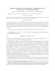
5. Numerical experiments In this section, we present several numerical experiments using synthetic and real data to illustrate that our LSB method can produce desirable image reconstruction results for the data detected from uniformly and sparsely distributed views and contaminated by the additive Gaussian white noise. Suppose that the projections from one view are uniformly spacing. Actually, this hypothesis is reasonable for the real tomography. All the involved algorithms other than FBP are programmed in C/C++ language and all the implementations ran on a desktop with Intel Xeon X5550 2.67GHz CPU, Fedora 11 OS and GCC 4.3.2 compiler, and no any parallel computing was conducted. 5.1. Comparisons with the FBP and the gradient-flow-based semiimplicit finite element method We first investigate the performance of our algorithm compared with the classical FBP and the gradient-flow-based semi-implicit finite element method (SFEM). For this numerical simulation, the test image is taken to be a synthetic Shepp-Logan phantom as shown in Fig. 5.1, which is discretized on a 257 × 257 pixel grid within the gray interval [0,1]. This phantom is often utilized in evaluating tomographic reconstruction algorithms. A set of uniformly spacing 257 parallel projections from each sampled view is obtained. The totally used angles is 60, namely, projecting once every 3◦ . Obviously, the sampling is severely insufficient. Then the additive Gaussian white noise is added onto the projection data from each view resulting in a set of corrupted data with signal-to-noise (SNR) (= 24.7dB), where the SNR in decibels is defined to be 2 ∑Mp np =1 P fnv ,np − P f nv =1 , ∑Nv ∑Mp 2 np =1 |εnv ,np − ε| nv =1

∑Nv SNR = 10log10

(5.1)

where Nv is the number of total angles, Mp is the number of total projections from each angle, P f is the average of totally noiseless measured data, ε is the added noise and ε is the average of ε. By Theorem 4.1, we recall that just the parameters β1 , β2 and α have effect on the convergence of our algorithm, and λ has impact on the reconstructed quality. Under this guidance, selecting these parameters is, hence, relatively easy. Here we choose the parameters λ = 0.1, β1 = 0.06, β2 = 3 × 10−5 , α = 10/3 in our algorithm. The iteration number is 1500. In addition, different filters (such as Ramp, Shepp-Logan, Hamming and Hann) and different interpolation schemes (such as nearest, linear, cubic spline) can be used in FBP. However, the performance of FBP has no evident improvement when we choose different combinations in terms of filters and interpolations. Without loss of generality, we only display in Fig. 5.1 the image reconstructed by FBP using a ramp filter and linear interpolating technique. In SFEM, we choose the modified parameter ϵ = 0.001, the temporal step size τ = 0.01 and regularization parameter λ = 2. The iteration number is 50 for the SFEM. As shown in Fig. 5.1, in terms of reconstruction quality, the LSB and the SFEM are much better than FBP; yet the SFEM is a little more blurry on edges than the LSB, which can be clearly figured out by Fig. 5.2. From the view of computational time, the new method is totally 73.8s for 1500 iterations, and the SFEM is about 1831s for 50 iterations, where the iterations are almost the least demanded steps for the two methods.

24


Fig. 5.1. The SNR = 24.7dB. From left to right, reconstructed images by FBP, the proposed method, SFEM, and the original image with gray scale over [0.0, 1.0].

Fig. 5.2. The cross sections of the images, as shown in Fig. 5.1, along the centers are plotted in the horizontal direction. The solid lines denote the cross sections of the original image. The dashed line and the dash-dotted line denote the cross sections of the reconstructed images by the SFEM (left) and the LSB (right), respectively.

5.2. Comparison with the gradient-descent-based split Bregman iteration As described in Subsection 2.2, we can directly apply the GDSB method to resolve the concerned optimization model (3.2). What is more, in this paper we have proved that the GDSB method is convergent under the proper condition. So why we do not use it but turn to propose the LSB method? The theoretical reason can be refer to Remark 4.8. The numerical aspect will be presented in this subsection. Here we consider a real CT image within the gray interval [0,1] as show in Fig. 5.3. The size of this image is also 257 × 257. We obtain uniformly spacing 257 parallel projections along each sampled view. The totally used views is 60. Then the additive Gaussian white noise is added onto the projection data along each view, which leads to a set of corrupted data with SNR= 29.6dB. As the size of the original image and the projection views are the same as the above experiment, so the parameters β1 , β2 and α can be selected as before to guarantee the LSB iterative convergence, namely, 0.06, 3 × 10−5 and 10/3, respectively. The regularization parameter λ is chosen as 1.0. In addition, we select the same λ as the LSB method to assure good reconstructed quality in the GDSB method. According to Theorems 4.1 and 4.6, to assure convergence of the GDSB method, we should sufficiently reduce the step size α for the relatively large λ replacing the small β2 in

C. CHEN AND G. XU

25

the convergence condition. Here the α = 2 × 10−6 , µ = 0.06. The rate of convergence of the GDSB method is, therefore, slower than that of the LSB method, which can be indicated by the decreasing amount of the objective energy as the iteration progressing as shown in Fig. 5.3.

Fig. 5.3. The star dashed and circle dash-dotted lines denote the values of the objective energy of the LSB and GDSB methods as the increase of the iteration number, respectively.

After 2000 iterations, the reconstructed images are shown in Fig. 5.4. It is easy to figure out that the performance of the LSB method is much better than that of the GDSB method. Remarkably, the latter introduces a lot of artifacts in the background, and leads to the blurry result. We further select another λ = 20 in both methods. Then, the LSB method produces the pretty near image as λ = 1, whereas the GDSB method is not convergent.

Fig. 5.4. The SNR = 29.6dB. From left to right, reconstructed images by the GDSB method, the LSB method with λ = 1, the LSB method with λ = 20, and the original image with gray scale over [0.0, 1.0].

6. Conclusions In this work, we have presented a novel linearized split Bregman iterative algorithm which is constructed by means of the thoughts of split and linearized Bregman

26


methods. We also have given the rigorous proof for the convergence of the proposed method under appropriate condition, where the convergence does not depend on the selection of the regularization parameter. Using the idea of the proof, we further proved the convergence of the GDSB method, yet which relies on the value of regularization parameter. In other words, our proposed method is more flexible and robust than the GDSB method. Notably, our method can be generalized to efficiently resolve the robust CS problem, as well as the TV-ℓ1 and ℓ1 -ℓ1 minimization problems. Finally, we have evaluated the performance of our algorithm in dealing with the sparse-view X-ray CT reconstruction problem using the synthetic and real data. As the results in these numerical comparisons, our algorithm yields high quality and almost accurate tomographic reconstructions in the above difficult problem. The numerical results presented in this paper also suggest that our algorithm greatly outperforms the classical FBP method in the reconstructed quality. Also, our algorithm possesses a bit better reconstructed performance and more effective than the earlier proposed SFEM method. Moreover, based on the numerical experiments, we can figure out that our method has much faster convergent rate and better reconstructed quality compared with the popular split Bregman method. Besides the advantages as the split Bregman method, such as efficient to solve several special ℓ1 problems, easy to program, simple to parallelize, saving memory, etc., our algorithm is more suitable for dealing with the general ℓ1 -regularized problems, for instance, the tomographic image reconstruction, and so forth. Acknowledgement. We would like to thank Prof. Chunlin Wu, from the School of Mathematical Sciences at Nankai University, for his helpful discussions, comments and corrections. We also want to thank Dr. Ming Li, from Institute of Computational Mathematics at Chinese Academy of Sciences, for his helpful suggestions on the part of numerical experiments.

REFERENCES [1] L. Bregman. The relaxation method of finding the common point of convex sets and its application to the solution of problems in convex programming. USSR computational mathematics and mathematical physics, 7(3):200–217, 1967. [2] J. Cai, S. Osher, and Z. Shen. Split Bregman methods and frame based image restoration. Multiscale Model. Simul., 8(2):337–369, 2009. [3] E. Cand` es. The restricted isometry property and its implications for compressed sensing. Comptes Rendus Mathematique, 346(9):589–592, 2008. [4] E. Cand` es, J. Romberg, and T. Tao. Robust uncertainty principles: Exact signal reconstruction from highly incomplete frequency information. IEEE Trans. Inform. Theory, 52(2):489– 509, 2006. [5] E. Cand` es, J. Romberg, and T. Tao. Stable signal recovery from incomplete and inaccurate measurements. Comm. Pure Appl. Math., 59(8):1207–1223, 2006. [6] E. Cand` es and M. Wakin. An introduction to compressive sampling. Signal Processing Magazine, IEEE, 25(2):21–30, 2008. [7] R. Chan, M Tao, and X. Yuan. Linearized Alternating Direction Method for Constrained Linear Least-Squares Problem. East Asian J. Appl. Math., 2(4):326–341, 2012. [8] T. Chan and S. Esedoglu. Aspects of total variation regularized l1 function approximation. SIAM J. Appl. Math., 65(5):1817–1837, 2005. [9] P. Charbonnier, L. Blanc-F´ eraud, G. Aubert, and M. Barlaud. Deterministic edge-preserving regularization in computed imaging. IEEE Trans. Image Process., 6(2):298–311, 1997. [10] C. Chen and G. Xu. Gradient-flow-based semi-implicit finite-element method and its convergence analysis for image reconstruction. Inverse Problems, 28(3):035006, 2012.

C. CHEN AND G. XU

27

[11] C. Chen and G. Xu. Computational inversion of electron micrographs using L2-gradient flows— convergence analysis. Math. Methods Appl. Sci., DOI: 10.1002/mma.2770, 2013. [12] A. Delaney and Y. Bresler. A fast and accurate fourier algorithm for iterative parallel-beam tomography. IEEE Trans. Image Process., 5(5):740–753, 1996. [13] A. Delaney and Y. Bresler. Globally convergent edge-preserving regularized reconstruction: an application to limited-angle tomography. IEEE Trans. Image Process., 7(2):204–221, 1998. [14] D. Donoho. Compressed sensing. IEEE Trans. Inform. Theory, 52(4):1289–1306, 2006. [15] E. Esser. Applications of Lagrangian-based alternating direction methods and connections to split Bregman. CAM report, 9:31, 2009. [16] B. Fahimian, Y. Zhao, R. Fung, Y. Mao, C. Zhu, Z. Huang, M. Khatonabadi, J. DeMarco, S. Osher, M. McNitt-Gray, and Miao J. Radiation dose reduction in medical CT through equally sloped tomography. Institute for Mathematics and Its Applications, 90095, 1770. [17] L. Feldkamp, L. Davis, and J. Kress. Practical cone-beam algorithm. JOSA A, 1(6):612–619, 1984. [18] H. Fu, M. Ng, M. Nikolova, and J. Barlow. Efficient minimization methods of mixed l2-l1 and l1-l1 norms for image restoration. SIAM J. Sci. Comput., 27(6):1881–1902, 2006. [19] R. Glowinski. Lectures on Numerical Methods for Non-Linear Variational Problems. Springer, 2008. [20] R. Glowinski and P. Le Tallec. Augmented Lagrangian and operator-splitting methods in nonlinear mechanics, volume 9. SIAM, 1989. [21] T. Goldstein, X. Bresson, and S. Osher. Geometric applications of the split Bregman method: segmentation and surface reconstruction. J. Sci. Comput., 45:272–293, 2010. [22] T. Goldstein and S. Osher. The split Bregman method for L1-regularized problems. SIAM J. Imaging Sci., 2(2):323–343, 2009. [23] E. Hale, W. Yin, and Y. Zhang. Fixed-point continuation for ℓ1 -minimization: Methodology and convergence. SIAM J. Optim., 19(3):1107–1130, 2008. [24] X. Han, J. Bian, E. Ritman, E. Sidky, and X. Pan. Optimization-based reconstruction of sparse images from few-view projections. Physics in Medicine and Biology, 57(16):5245, 2012. [25] R. Jia, H. Zhao, and W. Zhao. Convergence analysis of the Bregman method for the variational model of image denoising. Appl. Comput. Harmon. Anal., 27(3):367–379, 2009. [26] S. Ma, D. Goldfarb, and L. Chen. Fixed point and Bregman iterative methods for matrix rank minimization. Math. Program., 128(1-2):321–353, 2011. [27] M. Nikolova. Minimizers of cost-functions involving nonsmooth data-fidelity terms. application to the processing of outliers. SIAM J. Numer. Anal., 40(3):965–994, 2002. [28] S. Osher, M. Burger, D. Goldfarb, J. Xu, and W. Yin. An iterative regularization method for total variation-based image restoration. Multiscale Model. Simul., 4(2):460–489, 2005. [29] S. Osher and R. Fedkiw. Level set methods and dynamic implicit surfaces, volume 153. Springer, 2003. [30] S. Osher, Y. Mao, B. Dong, and W. Yin. Fast linearized Bregman iteration for compressive sensing and sparse denoising. arXiv preprint arXiv:1104.0262, 2011. [31] X. Pan, E. Sidky, and M. Vannier. Why do commercial CT scanners still employ traditional, filtered back-projection for image reconstruction? Inverse problems, 25(12):123009, 2009. [32] R. Rockafellar. Convex analysis, volume 28. Princeton university press, 1997. [33] L. Rudin, S. Osher, and E. Fatemi. Nonlinear total variation based noise removal algorithms. Phys. D, 60:259–268, 1992. [34] E. Sidky, J. Jørgensen, and X. Pan. Convex optimization problem prototyping for image reconstruction in computed tomography with the Chambolle–Pock algorithm. Physics in medicine and biology, 57(10):3065, 2012. [35] E. Sidky, C. Kao, and X. Pan. Accurate image reconstruction from few-views and limited-angle data in divergent-beam CT. Journal of X-ray Science and Technology, 14(2):119–139, 2006. [36] E. Sidky and X. Pan. Image reconstruction in circular cone-beam computed tomography by constrained, total-variation minimization. Physics in medicine and biology, 53(17):4777, 2008. [37] X. Tang, J. Hsieh, R. Nilsen, S. Dutta, D. Samsonov, and A. Hagiwara. A three-dimensionalweighted cone beam filtered backprojection (CB-FBP) algorithm for image reconstruction in volumetric CT–helical scanning. Physics in Medicine and Biology, 51(4):855, 2006. [38] C. Vogel and M. Oman. Iterative methods for total variation denoising. SIAM J. Sci. Comput., 17(1):227–238, 1996.

28


[39] G. Wang, T. Lin, P. Cheng, and D. Shinozaki. A general cone-beam reconstruction algorithm. IEEE Transactions on Medical Imaging, 12(3):486–496, 1993. [40] Y. Wang, J. Yang, W. Yin, and Y. Zhang. A new alternating minimization algorithm for total variation image reconstruction. SIAM J. Imaging Sci., 1(3):248–272, 2008. [41] C. Wu, J. Zhang, and X. Tai. Augmented Lagrangian method for total variation restoration with non-quadratic fidelity. Inverse Probl. Imaging, 5(1):237–261, 2011. [42] G. Xu, M. Li, A. Gopinath, and C. Bajaj. INVERSION OF ELECTRON TOMOGRAPHY IMAGES USING L2-GRADIENT FLOW—COMPUTATIONAL METHODS. J. Comput. Math., 29:501–25, 2011. [43] J. Yang and X. Yuan. Linearized augmented Lagrangian and alternating direction methods for nuclear norm minimization. Math. Comp., 82(281):301–329, 2013. [44] J. Yang and Y. Zhang. Alternating direction algorithms for ℓ1 -problems in compressive sensing. SIAM J. Sci. Comput., 33(1):250–278, 2011. [45] J. Yang, Y. Zhang, and W. Yin. An efficient TVL1 algorithm for deblurring multichannel images corrupted by impulsive noise. SIAM J. Sci. Comput., 31(4):2842–2865, 2009. [46] W. Yin, S. Osher, D. Goldfarb, and J. Darbon. Bregman iterative algorithms for ℓ1 minimization with applications to compressed sensing. SIAM J. Imaging Sci., 1(1):143–168, 2008.