gauge flavor symmetry is spontaneously (and completely) broken by the ... flavon interactions with the fermions determines the lepton mass matrices and mixing.
The little flavons F. Bazzocchi, S. Bertolini, and M. Fabbrichesi INFN, Sezione di Trieste and Scuola Internazionale Superiore di Studi Avanzati via Beirut 4, I-34014 Trieste, Italy
M. Piai
arXiv:hep-ph/0306184v3 16 Sep 2003
Department of Physics, Sloane Physics Laboratory University of Yale, 217 Prospect Street New Haven CT 06520-8120, USA (Dated: June 14, 2003) Fermion masses and mixing matrices can be described in terms of spontaneously broken (global or gauge) flavor symmetries. We propose a little-Higgs inspired scenario in which an SU (2) × U (1) gauge flavor symmetry is spontaneously (and completely) broken by the vacuum of the dynamically induced potential for two scalar doublets (the flavons) which are pseudo-Goldstone bosons remaining after the spontaneous breaking—at a scale between 10 and 100 TeV—of an approximate SU (6) global symmetry. The vacuum expectation values of the flavons give rise to the texture in the fermion mass matrices. We discuss in detail the case of leptons. Light-neutrino masses arise by means of a see-sawlike mechanism that takes place at the same scale at which the SU (6) global symmetry is broken. We show that without any fine tuning of the parameters the experimental values of the charged-lepton masses, the neutrino square mass differences and the Pontecorvo-Maki-Nakagawa-Sakata mixing matrix are reproduced. PACS numbers: 11.30.Hv, 14.60.Pq, 14.80.Mz
I.
MOTIVATIONS
Goldstone bosons are massless scalar particles remaining after the spontaneous breaking of global symmetries. Their number is determined by the number of broken generators in the group algebra. Goldstone bosons have no potential at all orders in perturbation theory and only couple derivatively to other fields. When the global symmetry is explicitly broken, the would-be-massless excitations acquire a potential and a mass proportional to the strength of the explicit breaking is generated. When two or more independent global symmetries are spontaneously broken by the same vacuum state, only the simultaneous explicit breaking of all symmetries lifts the flatness in the Goldstone boson potential. This property has been recently exploited in the little Higgs models [1] in order to stabilize against the one-loop quadratic renormalization the scalar potential of the Higgs fields that is responsible for electroweak symmetry breaking. Explicit breaking is arranged in such a way that more than one independent interaction term is needed in order to break all of the spontaneously broken global symmetries (collective breaking). As a result quadratic renormalization of the pseudoGoldstone boson masses arises only from the two-loop level. This makes it possible to increase by at least an order of magnitude the naturalness range of the massive scalar theory. In the standard model (SM) of electroweak interactions the natural cut off is raised from few TeV’s to few tens of TeV’s. This idea can be particularly attractive in a non-supersymmetric context in which elementary scalar fields are needed together with large scale differences between their masses and the theory cut off. A topical subject in which a scalar sector with hierarchical mass scales appears and the naturalness issue arises is flavor physics. The possibility that the hierarchy between the masses of the SM fermions arises because of some global horizontal symmetry acting on the three generations of matter fields has been extensively discussed in the literature [2, 3]. In most of these models, heavy scalar fields (referred to as flavons) carry the quantum numbers of this flavor symmetry, and are responsible for its breaking by acquiring non-vanishing vacuum expectation values (VEV’s). The Yukawa couplings of the SM are then generated from high-dimensional non-renormalizable operators which couple fermions, Higgs fields and flavons. The hierarchy between fermion masses is then the result of the hierarchy between the VEV’s and the cut-off scale of the theory which controls the magnitude of all non-renormalizable operators. Often, one is not interested in determining the scalar potential of the flavon sector itself, and simply assumes the existence of these VEV’s, with some hierarchical pattern deriving by unknown UV properties and details of the underlying theory. What we propose here is to obtain dynamically a stable (non-supersymmetric) scalar potential by assuming that the flavons are pseudo-Goldstone bosons originating from the breaking of an approximate global symmetry, spontaneously
broken to a subgroup containing the flavor symmetry that acts on the SM fermions. In this way, the field content of the flavon sector is determined. The gauging of the flavor symmetry breaks explicitly the global symmetry and induces a potential for the flavons. The form of the potential as well the size of the scalar couplings is obtained by means of the Coleman-Weinberg potential [4] of the non-linear sigma model describing the pseudo-Goldstone boson dynamics. The potential induced by gauge interactions preserves the SU (2)F × U (1)F flavor symmetry. The seed for the spontaneous breaking of the flavor symmetry is given by (gauge invariant) interactions of the two doublet flavons with right-handed neutrinos. These interaction terms destabilize the symmetric vacuum and drive the complete breaking of the local flavor symmetry. As a consequence all flavor mediating gauge bosons become massive. At the same time, the one-loop stability of the flavon masses on the broken vacuum is preserved. While this approach is quite general, in this paper we focus on the lepton sector of the SM. The structure of the flavon interactions with the fermions determines the lepton mass matrices and mixing. We show that all known mass and mixing parameters are reproduced without any fine tuning of the couplings of the model and that the needed patterns are derived from the vacuum structure of the two doublet flavon potential. We provide an explicit numerical example that gives an instance of normal hierarchy for the neutrino mass matrix and reproduces the PontecorvoMaki-Nakagawa-Sakata (PMNS) [6] mixing matrix as determined by the solar and atmospheric experiments—as well as the experimental charged-lepton masses. The same framework can be extended to the quark sector and together with issues related to CP violation will be the object of further work [5]. The flavon masses are stabilized against gauge induced quadratic renormalization at one-loop by a little-Higgs like mechanism [1] which will be described in detail in the next section. The general framework is similar to that discussed in ref. [7] and it actually uses the same high-energy global symmetry structure, albeit with a different pattern of gauge symmetry breaking. We have recalled this similarity in the naming of the flavons. II.
GOLDSTONE BOSONS
We choose as our basic flavor symmetry a gauged U (2)F ≃ SU (2)F × U (1)F . This choice is suggested by the approximate structure of the lepton sector: both neutrinos and charged-leptons can be classified in first approximation as two heavy flavor doublets—made by the τ and µ and the corresponding neutrinos—and two lighter singlets—the e and its neutrino. To exploit the features of the little Higgs models, at least two copies of the flavor group should be embedded in a larger (approximate) global symmetry. The request that the flavon sector exhibits a vacuum structure that allows for the complete breaking of the final gauge flavor symmetry is satisfied minimally by two flavon doublets. The smallest group that satisfies these requirements is SU (6), spontaneously broken to Sp(6), which has been discussed as a little Higgs model in ref. [7]. In our model we assume that the electroweak and flavor symmetries are embedded in two independent collectivebreaking frameworks with comparable cut-off scales ΛH ≃ ΛF ≃ Λ between 10 and 100 TeV. We will not enter the details of the ultraviolet completion of the model, and only deal with the general structure of the effective theory below the non-linear sigma model scale f = Λ/4π, where all the physics of flavor takes place. Consider then the spontaneous breaking of a global flavor symmetry SU (6) down to Sp(6). Fourteen of the generators of SU (6) are broken giving 14 (real) Goldstone bosons that can be written as a single field Σ = exp (iΠ/f ) Σ0 . They represent fluctuations around the (anti-symmetric) vacuum expectation value � � 0 −I . Σ0 ≡ hΣi = I 0
(1)
(2)
Within SU (6) we can identify four subgroups as SU (6) ⊃ [SU (2) × U (1)]2 .
(3)
We choose to gauge these subgroups, in such a way as to explicitly break the global symmetry through the gauge couplings. Only the diagonal combination of these gauge groups survives the spontaneous breaking of the symmetry so that we have [SU (2) × U (1)]2 → SU (2) × U (1) . We will use the latter groups to classify our fermion and flavon states.
(4)
SU (6)
Sp(6)
[SU (2) × U (1)]2 × U (1)P
[SU (2) × U (1)] × U (1)P
FIG. 1: Diagrammatic representation of the symmetry structure of the sigma model. Horizontal arrows indicate the spontaneous SU (6) → Sp(6) global symmetry breaking, vertical arrows the explicit breaking due to gauge interactions. A global U (1)P is preserved both by the spontaneous and the explicit breaking (induced by gauge interactions) while it is explicitly broken by the Yukawa sector of the model (see text).
The generators of the two SU (2) are given by the 6 × 6 matrices a σ 0 0 1 Qa1 = 0 0 0 2 0 0 0
(5)
and
0 0 0 1 Qa2 = 0 −σ a∗ 0 , 2 0 0 0
(6)
where σ a are the Pauli matrices; we choose the U (1)-charge matrices to be given by 1 Y1 = − √ diag [1, 1, −5, 1, 1, 1 ] 2 15 1 Y2 = − √ diag [1, 1, 1, 1, 1, −5 ] . 2 15
(7)
Contrary to [7], our U (1) charges belong to the generators of the group SU (6). Notice that the gauged subgroup [SU (2) × U (1)]2 has rank 4: this means that one of the generators of the Cartan sub-algebra of SU (6) (rank 5) is neither gauged nor explicitly broken. We identify this generator with P = diag [1, 1, 0, −1, −1, 0 ] ,
(8) 2
in such a way that it commutes with the whole gauge group [SU (2) × U (1)] , and it is orthogonal to all its generators. The generator P belongs to the algebra of Sp(6), and generates a U (1)P exact global symmetry of the sigma model we are discussing. This symmetry is then explicitly broken by the couplings of flavons to fermions, as we shall discuss. We summarize the symmetry structure of the sigma model in Fig 1. In the low-energy limit, there are two scalar bosons, � +� � 0� φ2 φ1 , (9) φ1 = and φ = 2 φ01 φ− 2 that are SU (2)-doublets with U (1) charges respectively 1/2 and −1/2, and one SU (2)- and U (1)- singlet s. The remaining four bosons are eaten in the breaking of the (gauge) [SU (2) × U (1)]2 symmetries. Accordingly we find that in the low-energy limit we can write the pseudo-Goldstone boson matrix as 0 0 φ+ 0 s φ02 1 0 0 φ01 −s 0 φ− 2 − 0∗ − 0 0 −φ2 −φ2 0 φ φ1 Π= 1 (10) . 0 −s∗ −φ0∗ 0 0 φ− 2 1 s∗ 0 −φ+ 0 0 φ0∗ 1 φ0∗ φ+ 2 2
2
0
φ+ 1
φ01
0
The singlet field becomes massive and has no expectation value in the vacuum configuration we will use; it is therefore effectively decoupled from the theory. The two doublets are our little flavons. Under the action of U (1)P global transformations U = exp (i αP ), the doublets and singlet transform as: φ1,2 −→ ei α φ1,2 ,
s −→ e2 i α s .
(11)
By construction, all Goldstone bosons start out massless and with only derivative couplings. However, as anticipated, the gauge and flavon-fermion interactions explicitly break the symmetry and give rise to an effective potential for the pseudo-Goldstones, the form of which allows for the existence of a non-symmetric vacuum that completely breaks the residual flavor gauge symmetry. III.
THE EFFECTIVE POTENTIAL
The effective lagrangian of the pseudo-Goldstone bosons below the symmetry-breaking scale is given by the kinetic term −
f2 ∗ Tr (Dµ Σ) (Dµ Σ) , 4
(12)
where the minus sign follows from the antisymmetric form of Σ. As already mentioned, we take the cut-off scale Λ = 4 πf to be of the order of 10-100 TeV. The absolute value of this scale is immaterial to the generation of the lepton mass matrices that, as we shall see, only depend on the ratio between the vacuum expectation values, which are proportional to f , and f itself. On the other hand, too large a scale would destabilize the standard model Higgs mass via interactions with the flavons and introduce a fine-tuning (we comment on this issue in Sect. IV). The covariant derivative in (12) is given by � � (13) + igi′ Biµ Yi Σ + ΣYiT Dµ Σ = ∂µ + igi Aaiµ Qai Σ + ΣQaT i
where Aaiµ and Biµ are the gauge bosons of the SU (2)i and U (1)i gauge groups respectively and Qai and Yi their generators as given in (5), (6) and (7). Since the vacuum Σ0 in eq. (2) breaks the symmetry (SU (2) × U (1))2 into the diagonal SU (2) × U (1), four combinations of the initial gauge bosons become massive; their masses are given by MA2 ′ =
(g12 + g22 )f 2 2
′
and MB2 ′ =
′
(g12 + g22 )f 2 . 4
(14)
The effective potential must break the SU (2) × U (1) remaining gauge symmetry and give mass to all surviving pseudo-Goldstone bosons, little flavons included. At one loop, the gauge interactions give rise to the ColemanWeinberg potential given by the two terms � � �� Λ2 3 M 2 (Σ) 2 4 Tr [M (Σ)] + Tr M (Σ) log + const. . (15) 16π 2 64π 2 Λ2 In agreement with the general framework of little Higgs models the quadratically divergent term gives mass only to the singlet fields s. No mass is generated for the (doublet) little flavons. In addition, a trilinear coupling between the doublets φ1 and φ2 and s and a quartic term for the two doublets are generated: 2 2 ! i ˜ † Λ2 i ˜ † 2 2 2 2 3 g1 s + , (16) Tr [M (Σ)] = f φ2 φ1 + 3 g2 s − φ2 φ1 16π 2 2f 2f where φ˜ = iσ2 φ∗ . From eq. (16) one obtains
m2s =
3 2 (g + g22 )f 2 , 2 1
(17)
and the quartic coupling † λ4 |φ˜2 φ1 |2 .
(18)
After integrating out the heavy singlet s, one obtains for λ4 the cut-off independent expression: λ4 =
g12 g22 ≃ O(g 2 ) , g12 + g22
(19)
which is the only term generated by the quadratic term in (15). This happens because of the mechanism of collective breaking for which the potential of the pseudo-Goldstone boson doublets (little flavons) is generated by the interplay of both gauge interactions, thus breaking explicitly the global SU (6) symmetry, while at the same time protecting the doublets from receiving a (quadratically divergent) mass at the one-loop level. Mass terms as well as other effective quartic couplings for the little flavons arise from the logarithmically divergent term in eq. (15). One can verify that the one-loop potential induced by gauge interactions includes the following terms µ21 φ†1 φ1 + µ22 φ†2 φ2 + λ1 (φ†1 φ1 )2 + λ2 (φ†2 φ2 )2 + λ3 (φ†1 φ1 )(φ†2 φ2 ) .
(20)
The size of the mass terms and effective couplings are given by MV2 3g 4 −2 < log (21) ∼ 10 , 64π 2 Λ2 where c are numerical coefficients, related to the expansion of the Σ, and MV is the mass of the massive gauge bosons (see, eq. (14)). The numerical estimate in eq. (21) takes into account that we take the (horizontal) gauge symmetry coupling to be of O(1). As we shall see, this follows from requiring the cut off of the model to be as low as possible (at a scale comparable with the SM little Higgs cut off) while avoiding too light flavons. In particular, we entertain the possibility of a flavor interaction cut off Λ ≃ 10 − 100 TeV and flavon masses just above the weak scale. Since λ4 , induced by the leading divergent term in the Coleman-Weinberg potential, turns out to be a sizeable coupling, other relevant contributions to the effective potential may arise from integration of the doublet self-interaction in eq. (18) which contributes to the λ1,2 terms with µ2i /f 2 ≃ λi ≃ c(µi , λi )
λ1,2 ≃
λ24 Λ2 −2 log 2 < ∼ 10 , 2 64π Mφ
(22)
which are in fact of the same order of those induced by the logarithmically divergent term in the gauge induced one-loop effective potential. The one-loop flavon potential generated by gauge interactions in eqs. (18)–(20) has to be compared with the general potential for two SU (2) doublets of opposite hypercharges that is given, up to four powers of the fields, by V4 (φ1 , φ2 ) = µ21 φ†1 φ1 + µ22 φ†2 φ2 + (µ23 φ˜†1 φ2 + H.c.) � � † + λ1 (φ†1 φ1 )2 + λ2 (φ†2 φ2 )2 + λ3 (φ†1 φ1 )(φ†2 φ2 ) + λ4 |φ˜†1 φ2 |2 + λ5 (φ˜1 φ2 )2 + H.c.
(23)
Depending on the sign of the determinant of the mass matrix of the scalar fields and on relationships among the various couplings, the potential in eq. (23) can have different symmetry breaking minima [8]. In particular we are interested to the vacuum which completely breaks the SU (2) × U (1) gauge flavor symmetry. The residual exact U (1)P global symmetry, acting with opposite charge on φi and φ˜i fields, forbids the generation of the µ3 and λ5 couplings. In the absence of µ23 and λ5 terms, the vacuum can be parametrized as � � � � 0 0 hφ1 i = hφ2 i = (24) v1 v2 with real VEV’s. The complete breaking of the flavor symmetry allows us to avoid the presence in the physical spectrum of massless flavor gauge bosons and is necessary in order to generate the lepton mass matrices. This vacuum breaks also the U (1)P symmetry, however a linear combination of P and flavor isospin is still preserved. The corresponding global symmetry U (1)P ′ , with P ′ = diag [1, 0, 0, −1, 0, 0 ] ,
(25)
is explicitly broken by the Yukawa sector. The requirement that the potential is bounded from below gives the three conditions λ1 + λ2 > 0,
4λ1 λ2 − λ23 > 0,
and λ4 − |λ5 | > 0 .
(26)
Assuming µ21,2 < 0 (and making use of µ23 = λ5 = 0) the symmetry breaking vacuum in eq. (24) leads to the following flavon mass spectrum m21,2 = m25,6 = 0 � 1 m23,4 = λ4 v12 + v22 2 q 2 m7,8 = λ1 v12 + λ2 v22 ± (λ1 v12 + λ2 v22 )2 − (4λ1 λ2 − λ23 )v12 v22 .
(27)
Positivity of the mass eigenvalues then requires λ4 > 0 and λ1 v12 + λ2 v22 > 0. The four massless degrees of freedom are eaten by the four gauge fields of the completely broken SU (2) × U (1) flavor symmetry which become massive at a scale determined by the VEV’s size v12 = −
2λ2 µ21 − λ3 µ22 4 λ1 λ2 − λ23
v22 = −
2λ1 µ22 − λ3 µ21 . 4 λ1 λ2 − λ23
(28)
The condition µ21 , µ22 < 0 can be realized if there exist fermions coupled to the doublets that induce contributions to the scalar masses of opposite sign with respect to that induced by gauge interactions. This role is played in the model by heavy right-handed Majorana neutrinos, with mass M ≃ f . Radiative contributions to the flavon potential arising from global SU (6) breaking couplings to Majorana right-handed neutrinos (as given in the next section) lead to scalar mass terms µ21,2 ≃ −c(1,2) ηn n
Λ2 ≃ −c(1,2) ηn f 2 , n 16π 2
(29)
(1,2)
where cn are coefficients of order unity. These quadratically-divergent corrections maintain the flavon mass scale −2 below the f scale (and in the TeV regime) as long as ηi < ∼ 10 . Thus, still avoiding a large fine tuning of the couplings, no collective breaking mechanism is required for the lepton-induced renormalization (the only large couplings in the model are gauge and the Yukawa of the top quark). Notice that, the contributions to the quartic couplings induced by the massive right-handed neutrinos are therefore given by (1,2,3)
λ1,2,3 ≃
Λ2 cnm ηn ηm −6 log 2 < ∼ 10 2 16π M
(30)
and are subleading, with respect to those induced by gauge interactions. From eq. (28) and eqs. (21)–(29) we obtain v1 , v2 = O(f ), which in turn implies that the four flavor gauge bosons and two of the flavon states have masses of order f , while the remaining two scalars have masses of O(10−1 f ). As anticipated, considering the lightest flavon states to be in the weak scale range puts the flavor cut off Λ = 4πf in the 10 − 100 TeV regime, in the same ballpark of the SM little-Higgs cut off. Assuming all of the above conditions satisfied (we will not be concerned with the detail of the ultraviolet completion of the theory) we now discuss the neutrino and charged lepton mass textures that arise by assigning non-trivial flavor transformation properties to the lepton families. IV.
COUPLING FLAVONS TO LEPTONS
We classify leptons of different families according to the [SU (2) × U (1)]2 gauge flavor symmetry. As we have seen, the spontaneous breaking of the global SU (6) → Sp(6) (approximate) symmetries leads to the [SU (2) × U (1)]2 → SU (2) × U (1) breaking. We let all fermions to transform under only one of the initial SU (2) × U (1) groups, so that their charges will coincide with those of the surviving diagonal group. This choice determines the possible terms appearing in the flavon interactions. We will indicate the remaining SU (2) × U (1) flavor symmetry with the index F to distinguish it from the electroweak group. In the following, all Greek indices belong to the flavor group while Latin indices refer to the electroweak group. We assume all the fermions to be neutral under U (1)P . The standard model electron doublet leL is an SU (2)F singlet charged under U (1)F , while lµ,τ L are members of a doublet, that is l1L = leL ,
YF = −2 ;
LL = (lµ , lτ )L ,
YF =
1 ; 2
(31)
where we have written explicitly the flavor hypercharge. Right-handed charged leptons have a similar structure eR ,
YF = 1;
ER = (µ , τ )R ,
YF =
1 . 2
(32)
i In order to have a see-saw -like mechanism [10], we introduce three right-handed neutrino νR which are SU (2)F singlets :
ν1R ,
YF = 1 ;
ν2R ,
YF = −1 ;
ν3R ,
YF = 0 .
(33)
TABLE I: Summary of the charges of all leptons and the relevant component of the pseudo-Goldstone bosons under the horizontal flavor groups SU (2)F and U (1)F . α = 2, 3 leL eR LL = (lµ , lτ )L ER = (µ , τ )R ν1R ν2R ν3R Σα−1 6 Σα−1 3 Σ3 2+α Σ6 2+α
= (−i/f = (+i/f = (−i/f = (−i/f
φ1 + ...)α φ2 + ...)α φ∗1 + ...)α φ∗2 + ...)α
U (1)F −2 1 1/2 1/2 1 −1 0
SU (2)F 1 1 2 2 1 1 1
1/2 −1/2 −1/2 1/2
2 2 2∗ 2∗
This choice allows us to have in the effective lagrangian Majorana mass entries at the scale M ∼ f . The physical PMNS mixing is generated thanks to the different assignments of right-handed charged leptons and neutrinos, which give different textures to the charged lepton mass matrix, the Dirac mass matrix of neutrinos and the (non-trivial) Majorana mass matrix of right-handed neutrinos. Taking into account the charge assignments, as summarized in Table I, we construct the Yukawa interactions by coupling, in a gauge invariant manner, the leptons to the pseudo-Goldstone bosons Σ and to the standard-model Higgs boson. At the first non-trivial order in powers of the Σ fields we have: h Lν = λ1ν ν1R (Σα−1 6 Σ6 2+α )−Y1L +Yν1R + λ2ν ν2R (Σα−1 6 Σ6 2+α )−Y1L +Yν2R i −Y +Y ˜ † l1L ) + λ3ν ν3R (Σα−1 6 Σ6 2+α ) 1L ν3R (H h + i ν1R (λ′1ν ǫαβ Σβ−1 6 + λ′′1ν Σ6 2+α ) + ν2R (λ′2ν ǫαβ Σβ−1 3 + λ′′2ν Σ3 2+α ) (Σδ−1 6 Σ6 2+δ ) i ˜ † lαL ) + ν3R (λ′3ν ǫαβ Σβ−1 3 + λ′′3ν Σ3 2+α ) (H � � � η1 f η2 f M c ν c + Σα−1 6 Σ3 2+α + Σα−1 3 Σ6 2+α ν1R + − 2R + ν2R ν1R 2 2 2 � � � η4 f M3 η3 f c ν + Σα−1 6 Σ3 2+α + Σα−1 3 Σ6 2+α ν3R + − 3R 2 2 2 η5 f η6 f c ν c ν (Σα−1 6 Σ6 2+α )†2 ν1R (Σα−1 6 Σ6 2+α )2 ν2R + (34) 1R + 2R 2 2 � η8 f � η7 f c ν c c ν c (Σα−1 6 Σ6 2+α )† ν1R (Σα−1 6 Σ6 2+α ) ν2R + 3R + ν3R ν1R + 3R + ν3R ν2R + H.c. , 2 2
˜ = iσ2 H ∗ , and where ǫ = iσ2 is the completely antisymmetric tensor with indices α, β = 2, 3 (2 → µ, 3 → τ ), H c T ¯ ψ = Cψ . Analogously, for the charged leptons we have h i Le = eR λ1e (Σα−1 6 Σ6 2+α )(−Y1L +Y1R ) (H † l1L ) + i (λ3e Σ6 2+α + λ2e ǫα β Σβ−1 6 )(H † lαL ) h i + EαR i (λ′1E Σ6 2+α + λ1E ǫα β Σβ−1 6 ) (Σδ−1 6 Σ6 2+δ )−Y1L (H † l1L ) h � + EαR δα β − λ2E + λ′2E Σγ−1 6 Σ3 2+γ + λ′′2E Σγ−1 3 Σ6 2+γ � � + λ3E Σα−1 6 Σ3 2+β + λ′3E ǫα δ ǫβ γ Σ6 2+δ Σγ−1 3 + (3 ↔ 6) � �i + λ4E Σα−1 6 Σγ−1 3 ǫβ γ + λ′4E ǫα δ Σ6,2+δ Σ3,2+α + (3 ↔ 6) (H † lβL ) + H.c. . (35)
In eqs. (35)–(35) we have not included terms ǫγ δ Σγ−1 6 Σδ−1 3 = φ˜†1 φ2 /f 2 +... which vanish on the vacuum of eq. (24) and do not contribute to the fermion masses. The U (1)P symmetry is explicitly broken by the lepton Yukawa couplings. The leading breaking is due to the terms linear in φ˜1 and φ2 which arise from the terms linear in the Σ fields in eq. (35). On the other hand, these U (1)P violating terms have a negligible impact on the flavon potential: as it will be clear from the section devoted to the numerical discussion of the mass matrices and mixing, none of the Yukawa parameters entering the lagrangian is large (typically they are of the order of 10−2 or less). As a consequence, the µ23 terms—quadratically divergent contributions notwithstanding (two-loops are needed above the electroweak symmetry breaking scale)—turn out to be negligible with respect to µ21,2 . Analogously flavon-Higgs mixing terms of the type H † Hφ†i φi —induced at one-loop by combinations of lepton Yukawa couplings—do not destabilize the electroweak breaking as long as we consider flavon vacuum expectation values below 10 TeV together with Yukawa couplings of the order of 10−2 or less. In our approach right-handed neutrinos are integrated out at the f scale thus realizing a low-energy see-saw mechanism (similar realizations have been recently proposed in the context of extended technicolor [11] and deconstruction [12]). The Dirac and Majorana matrices combine yielding below the f scale effective Yukawa couplings of the form: � � c H ˜ ∗ )(H ˜ † lτ L ) MTRL (Σ)M−1 (Σ)MRL (Σ) (36) (lρL RR ρτ where lτc L = (ντc , ecτ )L and τ, ρ = 1, 2, 3. Taking the leading non-vanishing orders in M−1 RR (Σ) and in the number of Σ fields we obtain:
c H ˜ ∗ )(H ˜ † l1L ) � � (l1L −2Y 2λ1ν λ2ν + r λ23ν [Σα−1 6 Σ6 2+α ] 1L M ˜ ∗ )(H ˜ † lαL ) + (lc H ˜ ∗ )(H ˜ † l1L ) (lc H −Y +Y αL λ2ν (λ′1ν ǫαβ Σβ−1 6 + λ′′1ν Σ6 2+α ) [Σδ−1 6 Σ6 2+δ ] 1L ν2R + 1L M ˜ ∗ )(H ˜ † lβL ) � (lc H (iσ2 στ )α β (iσ2 στ )δ γ (λ′3ν )2 Σδ−1 3 Σγ−1 3 + αL 2M3 � ′ ′′ + λ3ν λ3ν (ǫγγ ′ Σδ−1 3 Σ3 2+γ ′ + δ ↔ γ) + (λ′′3ν )2 ǫδδ′ ǫγγ ′ Σ3 2+δ′ Σ3 2+γ ′ + H.c. , (37)
− 2 Lν =
where r = M/M3 , στ /2 are the generators of the SU (2)f gauge group (τ = 1, 2, 3). At the leading order in the pseudo-Goldstone boson expansion the effective Yukawa lagrangian is given by !4 † c H ˜ ∗ )(H ˜ † l1L ) � � (l φ φ 1 − 2 Lν = 2λ1ν λ2ν + r λ23ν 1L − 22 M f " c H ˜ ∗ )(H ˜ † LL ) iσ2 (λ′ φ1 − λ′′ φ˜2 ) (l1L 1ν 1ν + λ2ν M f # ! ˜ ∗ )(H ˜ † l1L ) φ†2 φ1 (λ′1ν φ1 − λ′′1ν φ˜2 )T iσ2T (LcL H − 2 + f M f � � ˜ ∗ )T (iσ2 στ )(H ˜ † LL )T h (LcL H ′ 2 T ′ ′′ ˜T iσ2 στ φ2 + φ2 T iσ2 στ φ˜1 φ + −(λ ) φ iσ σ φ + λ λ 2 τ 2 1 3ν 2 3ν 3ν 2M3 f 2 i − (λ′′3ν )2 φ˜T1 iσ2 στ φ˜1 + H.c.
where we have used a compact notation for the flavor doublets (transposition acts on flavor indices). Analogously, for the charged leptons from eq. (35) one obtains " # !3 † ˜2 ) φ φ φ iσ (λ φ − λ 1 2 2e 1 3e − Le = eR − λ1e (H † l1L ) − 2 2 + (H † LL ) f f " !2 # ′ ˜2 ) φ† φ1 T iσ2 (λ1E φ1 − λ1E φ + ER − 22 (H † l1L ) f f � ! ! � " † ′ ˜2 φ˜† + (1, +) ↔ (2, −) † † λ φ φ − λ φ 13E 1 2 1 23E φ2 φ2 φ1 φ1 T − λ′′2E + + ER λ2E + λ′2E f2 f2 f2
(38)
�# � λ14E φ1 φ˜†2 − λ′24E φ˜2 φ†1 + (1 ↔ 2) (H † LL )T + H.c. , − f2
(39)
where transposition acts on flavor indices. A.
Mass matrices
When the SU (2)F × U (1)F is broken, the little flavons assume their expectation values v1 ≃ v2 ≃ εf and we are left with the left-handed neutrino and charged-lepton mass matrices. At the lowest order in ε, factoring out a common coefficient λ′3ν in the leading terms and assuming all the other Yukawa couplings to be equal we obtain from eq. (38) the mass matrix for the neutrinos 0 0 0 2 hh0 i 2 Mν = λ′2 ε 0 1 1. (40) 3ν M3 0 1 1 In a similar manner, from the lagrangian (39) after factoring charged-lepton matrix yields 0 Ml = λ2E hh0 i 0 0 The coefficient
2 λ′2 3ν
out the coefficient λ2E of the leading terms in the 0 0 1 0. 0 1
(41)
hh0 i2 2 ε = mντ M3
(42)
normalizes the absolute value of the matrix entries and fixes the value of the Yukawa coupling λ′3ν . The scale M is just below or around f and therefore we are not implementing the usual see-saw mechanism that requires scales as large as 1013 TeV. Therefore, neutrino masses are in this model small because of the smallness of the corresponding effective Yukawa coupling λ′3ν that we take—for M ≃ M3 ≃ 10 TeV—of the order of 10−4 . This value is necessary to give the correct absolute values for the square mass differences and it cannot be explained by the model; what the model explains is the hierarchy among the masses of different families. We estimate the coefficient λ2E by means of value of the mass of the τ lepton in the relation λ2E hh0 i ≃ mτ ,
−2
(43)
which yields a value for λ2E of about 10 . The form of the mass matrices thus obtained is encouraging because it shows a texture leading to normal hierarchy and maximal mixing in the neutrino sector as well as a first approximation to the charged-lepton masses. However, this result is not sufficient as it stands because the mixing angles and masses depends in a critical manner on the exact values of all the entries. For instance, if we were to take the matrices (40) and (41) as they stand, they would lead to a diagonal mixing matrix. While what we have found is a potentially correct texture, in order to reproduce the experimental data, it must have entries that are not equal even though they must, at the same time, only differ by O(1) coefficients. This result is achieved by taking a closer look at the model. Before that, we pause to briefly comment on the problems of gauge anomalies and of the experimental bounds for the flavon masses. B.
Anomaly cancellation
Gauge anomalies are potentially present in the theory, as it can be easily seen by inspection considering the charges of the matter fields. They arise from five kinds of triangle diagrams, that in the presence of leptons alone yields: SU (2)F,EW × SU (2)F,EW × U (1)F → Tr YF = −4 67 U (1)F × U (1)F × U (1)F → Tr YF3 = − 4 5 2 = −3
2 U (1)F × U (1)EW × U (1)EW → Tr YF YEW =−
U (1)F × U (1)F × U (1)EW → Tr YF2 YEW
× H
µL
× H
eL
φ1,2 eR
×
××× φ
eR
×
FIG. 2: Flavon mediated contribution to the decay µ → e e e
While a discussion of the anomalies cannot be done until also the quark fields are included and their charges with respect to the flavor gauge symmetries known, we notice that whatever anomaly is eventually found, it can be canceled by a Wess-Zumino term. Since all the anomalous gauge symmetries are spontaneously broken, it is possible to build the required Wess-Zumino term by means of only the would-be-Goldstone bosons that are eventually eaten by the gauge fields. As shown in [9] this construction is sufficient to cancel all gauge anomalies (as well as those from gravity) without having to modify the matter content of the theory or strongly affecting the low-energy phenomenology. C.
Bounds on the flavon masses
The most severe bounds on the little flavon interactions and masses, in the context of the present discussion, come from tightly constrained lepton-number violating processes like µ → eγ and µ → 3 e. On the other hand, the inspection of the vertices involved in diagrams with flavon exchange (lepton exchange can be safely neglected) shows that a combination of loops, couplings and flavon multiplicity severely suppresses the decay rates. For instance, at the tree level, we estimate from eq. (39) that the branching ratio for µ → 3e is (see fig. (2)) BR(µ → 3e) < N 2
�
λ1e λ2e,3e 2 gW
�2 �
hh0 i f
�4 �
v1 v2 f2
�5 �
mW mφ
�4
≃ 10−10
�
hh0 i f
�4 �
mW mφ
�4
,
(44)
where N is a combinatorial factor of order 10, the Yukawa couplings λie are all of order 10−2 or less, and, as we shall see in the numerical analysis, v1 v2 /f 2 is of order 10−1 . The present experimental bound of 10−12 thus allows for the existence of light flavons. In the range of scales under consideration, inspection of flavor gauge mediated contributions does not show the presence of large effects either. We postpone a more detailed discussion of little flavon phenomenology to a forthcoming paper. V.
LEPTON MASSES AND MIXING
The more complete analysis requires that the first non-vanishing entries in all matrix elements be kept. In addition, we also retain O(ε2 ) corrections to all leading entries—that means O(ε4 ) terms in the neutrino mass matrix and O(ε2 ) terms in the charged lepton case. The two vacua are distinguished as v1 = f ε1 and v2 = f ε2 . This analysis gives us the full textures. Accordingly, the neutrino Majorana mass matrix can now be written as hh0 i2 Mν = M
�
�
r λ2 + 2λ1ν λ2ν ε4 ε4 1 2 3ν −λ2ν λ′ ε2 ε2 1ν 1 −λ2ν λ′′ ε1 ε2 1ν 2
−λ2ν λ′ ε2 ε2 1ν 1 ′2 r λ ε2 ρ + 2λ′ λ′ ε2 ε2 3ν 2 1ν 2ν 1 2 r λ′ λ′′ ε1 ε2 ρ + λ′ λ′′ ε3 ε2 + λ′ λ′′ ε1 ε3 3ν 3ν 1ν 2ν 1 2ν 1ν 2
−λ2ν λ′′ ε1 ε2 1ν 2 ′ ′′ r λ λ ε ε ρ + λ′ λ′′ ε3 ε2 + λ′ λ′′ ε1 ε3 3ν 3ν 1 2 1ν 2ν 1 2ν 1ν 2 r λ′′2 ε2 ρ + 2λ′′ λ′′ ε2 ε2 3ν 1 1ν 2ν 1 2
!
,
(45)
where ρ ≡ 1 − ε21 /3 − ε22 /3 comes from the expansion of the Σ field. The eigenvalues of this matrix are the masses of the three neutrinos. In the same approximation, the Dirac mass matrix for the charged leptons is given by
Ml = hh0 i
λ1e ε3 ε3 1 2 λ1E ε2 ε3 1 2 λ′ ε3 ε2 1E 1 2
λ2e ε1 λ2E + (λ′ + λ′ ) ε2 − (λ′′ + λ′ ) ε2 1 2 2E 13E 2E 23E −(λ14E + λ24E ) ε1 ε2
λ3e ε2 (λ′ + λ′ ) ε1 ε2 14E 24E λ2E + (λ′ + λ13E ) ε2 − (λ′′ + λ23E ) ε2 1 2 2E 2E
!
.
(46)
The 3 × 3 unitary PMNS mixing matrix [6] for the leptons is defined as U = Ul† Uν where Uν , Ul are the neutrino and charged lepton mixing matrices defined, respectively, by �2 and Uν† Mν Uν = MD Ul† M†l Ml Ul = MD ν , l
(47)
(48)
D where MD l and Mν are the diagonal mass matrices for, respectively, charged and neutral leptons. We use for U the standard parametrization (in the case of a real matrix)
c12 c13 c13 s12 s13 U = −c23 s12 − c12 s12 s23 c12 c23 − s12 s13 s23 c13 s23 , −c12 c23 s13 + s12 s23 −c23 s12 s13 − c12 s23 c13 c23
(49)
where sij = sin θij and cij = cos θij and thus obtain a U parametrized by three angles. The mass matrices (45) and (46) necessarily contain many parameters. The coupling strengths in front of the various Yukawa terms of the lagrangian can be different for different flavors and different interactions and we have kept them distinguished so far. For the model to be natural, these parameters must be roughly of the same order once their overall values have been fixed by eq. (42) and (43) respectively. A.
Experimental data
Let us briefly review the experimental results. Compelling evidences in favor of neutrino oscillations and, accordingly of non-vanishing neutrino masses has been collected in recent years from neutrino experiments [13]. Combined analysis of the experimental data show that the neutrino mass matrix is characterized by a hierarchy with two square mass differences (at 99.73% c.l.): ∆m2⊙ = (3 − 35) × 10−5 eV2
|∆m2⊕ | = (1.4 − 3.7) × 10−3 eV2 ,
(50)
the former controlling solar neutrino oscillations [14] and the latter the atmospheric neutrino experiments [15]. In the context of three active neutrino oscillations, the mixing is described by the PMNS mixing matrix U in eq. (49). Such a matrix is parameterized by three mixing angles, two of which can be identified with the mixing angles determining solar [14] and atmospheric [15] oscillations, respectively (again, at 99.73% c.l.): tan2 θ⊙ = 0.25 − 0.88 , sin2 2 θ⊕ = 0.8 − 1.0 .
(51)
For the third angle, controlling the mixing ντ -νe , there are at present only upper limits, deduced by reactor neutrino experiments [16] (at 95% c.l.): sin2 θ < 0.09 .
(52)
Finally, the charged-lepton masses are well known and given by mτ ≃ 1770 MeV, mµ ≃ 106 MeV and me ≃ 0.5 MeV, respectively—so that, mτ /mµ ≃ 17 and mµ /me ≃ 207. B.
Numerical results
The goal of our numerical analysis is to show that, in spite of the many undetermined couplings in eq. (45) and eq. (46), the known pattern of mixing angles and neutrino mass differences is rather well reproduced by setting all the ratios of Yukawa couplings—remaining after extracting the overall factors in eqs. (40)–(41)—equal to 1. The textures induced by the structure of the flavon VEV’s already determine the desired result. Just considering variation of O(1) of a few couplings allows for the complete fit of all lepton masses. We argue therefore that the model reproduces quite naturally the known structure of the leptonic spectrum. Let us then—after having fixed the overall factors by eqs. (42)–(43)—keep as input parameters of the theory the vacuum values v1 = ε1 f and v2 = ε2 f while taking all ratios of Yukawa couplings and r equal in modulus to 1. This procedure leaves us with only two parameters in terms of which we may write the following toy mass matrices:
3 ε41 ε42 −ε21 ε2 −ε1 ε22 hh0 i Mν = λ′2 ε22 ρ + 2 ε21 ε22 ε1 ε2 ρ + ε31 ε2 + ε1 ε32 −ε21 ε2 3ν M3 ε21 ρ + 2ε21 ε22 −ε1 ε22 ε1 ε2 ρ + ε31 ε2 + ε1 ε32 2
and
ε31 ε32 ε1 ε2 Ml = λ2E hh0 i ε21 ε32 1 2ε1 ε2 . ε31 ε22 2ε1 ε2 1
(53)
(54)
At this point we can vary our two parameters to find the best fit. We take the range for ε1 and ε2 between 0.1 and 1 in such a way that we do not introduce large VEV’s hierarchies. As an example, for the representative values: ε1 ≃ 0.1 and ε2 ≃ 0.8 , we obtain for the mixing angles tan2 θ⊙ ≃ 0.9 , sin2 2 θ⊕ ≃ 1 , sin2 θ ≃ 0.006 ,
(55)
∆m212 /∆m223 ≃ 0.005 ,
(56)
mτ /mµ ≃ 1.6 and mτ /me ≃ 3470 .
(57)
for the neutrino normal-hierarchy ratio
and for the charged-lepton mass hierarchy
Albeit using a very rough approximation, we find values for the mixing angles and neutrino masses in the ballpark of the experimental values, with the exception of the µ mass; this is to be expected since µ and τ start out as members of a SU (2)F doublet and their splitting must come from the detailed values of the Yukawa couplings. As a matter of fact, in order to fit correctly all data, it is enough to consider the case in which some of the Yukawa couplings in the Dirac mass matrix (46) differ by O(1) coefficients. We have checked that this is possible, as a matter of fact, with just two more parameters. Therefore, without introducing any large ratio among Yukawa couplings or VEV’s, all the known experimental data for the lepton masses and mixing are reproduced. Acknowledgments
It is a pleasure to thank M. Frigerio, E. Pallante and S. Petcov for discussions. One of us (MP) also thanks T. Appelquist and W. Skiba for discussions and SISSA for the hospitality. This work is partially supported by the European TMR Networks HPRN-CT-2000-00148 and HPRN-CT-2000-00152. The work of MP is supported in part by the US Department of Energy under contract DE-FG02-92ER-40704.
[1] N. Arkani-Hamed, A. G. Cohen, E. Katz and A. E. Nelson, JHEP 0207, 034 (2002) [arXiv:hep-ph/0206021]; I. Low, W. Skiba and D. Smith, Phys. Rev. D 66, 072001 (2002) [arXiv:hep-ph/0207243]; D. E. Kaplan and M. Schmaltz, arXiv:hep-ph/0302049. S. Chang and J. G. Wacker, arXiv:hep-ph/0303001. W. Skiba and J. Terning, arXiv:hep-ph/0305302. S. Chang, arXiv:hep-ph/0306034. [2] H. Harari, H. Haut and J. Weyers, Phys. Lett. B 78, 459 (1978). C. D. Froggatt and H. B. Nielsen, Nucl. Phys. B 147, 277 (1979). T. Maehara and T. Yanagida, Prog. Theor. Phys. 61, 1434 (1979). G. B. Gelmini, J. M. Gerard, T. Yanagida and G. Zoupanos, Phys. Lett. B 135, 103 (1984).
[3] A partial, and by no means complete list includes the following works: M. Dine, R. G. Leigh and A. Kagan, Phys. Rev. D 48, 4269 (1993) [arXiv:hep-ph/9304299]. M. Leurer, Y. Nir and N. Seiberg, Nucl. Phys. B 398, 319 (1993) [arXiv:hep-ph/9212278]; Nucl. Phys. B 420, 468 (1994) [arXiv:hep-ph/9310320]. P. Pouliot and N. Seiberg, Phys. Lett. B 318, 169 (1993) [arXiv:hep-ph/9308363]. D. B. Kaplan and M. Schmaltz, Phys. Rev. D 49, 3741 (1994) [arXiv:hep-ph/9311281]. L. J. Hall and H. Murayama, Phys. Rev. Lett. 75, 3985 (1995) [arXiv:hep-ph/9508296]. A. Pomarol and D. Tommasini, Nucl. Phys. B 466, 3 (1996) [arXiv:hep-ph/9507462]; R. Barbieri, G. R. Dvali and L. J. Hall, Phys. Lett. B 377, 76 (1996) [arXiv:hep-ph/9512388]; P. H. Frampton and O. C. Kong, Phys. Rev. Lett. 77, 1699 (1996) [arXiv:hep-ph/9603372]. E. Dudas, C. Grojean, S. Pokorski and C. A. Savoy, Nucl. Phys. B 481, 85 (1996) [arXiv:hep-ph/9606383]. P. Binetruy, S. Lavignac and P. Ramond, Nucl. Phys. B 477, 353 (1996) [arXiv:hep-ph/9601243]. R. Barbieri, L. J. Hall, S. Raby and A. Romanino, Nucl. Phys. B 493, 3 (1997) [arXiv:hep-ph/9610449]; G. Altarelli and F. Feruglio, Phys. Rept. 320, 295 (1999). H. Fritzsch and Z. z. Xing, Prog. Part. Nucl. Phys. 45, 1 (2000) [arXiv:hep-ph/9912358]. Z. Berezhiani and A. Rossi, Nucl. Phys. B 594, 113 (2001) [arXiv:hep-ph/0003084]; A. Masiero, M. Piai, A. Romanino and L. Silvestrini, Phys. Rev. D 64, 075005 (2001) [arXiv:hep-ph/0104101]. M. Frigerio and A. Y. Smirnov, Nucl. Phys. B 640, 233 (2002) [arXiv:hep-ph/0202247]. [4] S. R. Coleman and E. Weinberg, Phys. Rev. D 7, 1888 (1973). [5] F. Bazzocchi et al., to appear. [6] B. Pontecorvo, Sov. Phys. JETP 6 (1958) 429; Z. Maki, M. Nakagawa and S. Sakata, Prog. Theor. Phys. 28 (1962) 870. [7] I. Low, W. Skiba and D. Smith , in [1] [8] M. Sher, Phys. Rept. 179, 273 (1989). [9] M. Fabbrichesi, R. Percacci, M. Piai and M. Serone, Phys. Rev. D 66, 105028 (2002) [arXiv:hep-th/0207013]. [10] T. Yanagida, in Unified Theory and Baryon Number, Tsukuba, 1979; M. Gell-Mann, P. Ramond and R. Slansky, in Supergravity, edited by P. van Nieuwehuizen and O. Freedman (NorthHolland, Amsterdam 1979), p. 317; R. N. Mohapatra and G. Senjanovic, Phys. Rev. Lett. 44, 912 (1980). [11] T. Appelquist and R. Shrock, Phys. Lett. B 548, 204 (2002) [arXiv:hep-ph/0204141]. [12] K. R. S. Balaji, M. Lindner and G. Seidl, arXiv:hep-ph//0303245. [13] Y. Fukuda et al. [Super-Kamiokande Collaboration], Phys. Rev. Lett. 81, 1562 (1998) [arXiv:hep-ex/9807003]; S. Fukuda et al. [Super-Kamiokande Collaboration], Phys. Rev. Lett. 86, 5656 (2001) [arXiv:hep-ex/0103033]; S. Fukuda et al. [Super-Kamiokande Collaboration], Phys. Rev. Lett. 86, 5651 (2001) [arXiv:hep-ex/0103032]; Q. R. Ahmad et al. [SNO Collaboration], Phys. Rev. Lett. 87, 071301 (2001) [arXiv:nucl-ex/0106015]; Q. R. Ahmad et al. [SNO Collaboration], Phys. Rev. Lett. 89, 011301 (2002) [arXiv:nucl-ex/0204008]; M. H. Ahn et al. [K2K Collaboration], Phys. Rev. Lett. 90, 041801 (2003) [arXiv:hep-ex/0212007]; K. Eguchi et al. [KamLAND Collaboration], Phys. Rev. Lett. 90, 021802 (2003) [arXiv:hep-ex/0212021]. [14] See, for instance: S. Choubey, A. Bandyopadhyay, S. Goswami and D. P. Roy, arXiv:hep-ph/0209222. [15] See, for instance: G. L. Fogli, E. Lisi, A. Marrone and D. Montanino, arXiv:hep-ph/0303064. [16] M. Apollonio et al. [CHOOZ Collaboration], Phys. Lett. B466 (1999) 415 (hep-ex/9907037); F. Boehm, J. Busenitz et al., Phys. Rev. Lett. 84 (2000) 3764 and Phys. Rev. D62 (2000) 072002.