The log-generalized modified Weibull regression model - IME-USP

bjps bjps v.2009/10/20 Prn:2009/12/07; 8:43

1

F:bjps110.tex; (Emilija) p. 1

Brazilian Journal of Probability and Statistics 2009, Vol. 0, No. 00, 1–29 DOI: 10.1214/09-BJPS110 © Brazilian Statistical Association, 2009

1

2 3

2

The log-generalized modified Weibull regression model

4 5

3 4

Edwin M. M.

Ortegaa ,

Gauss M.

Cordeirob

and Jalmar M. F.

Carrascoc

5

6

a Departamento de Ciências Exatas, ESALQ—USP

6

7

b Departamento de Estatística e Informática, DEINFO—UFRPE c Departamento de Estatística, IME—USP

7

Abstract. For the first time, we introduce the log-generalized modified Weibull regression model based on the modified Weibull distribution [Carrasco, Ortega and Cordeiro Comput. Statist. Data Anal. 53 (2008) 450–462]. This distribution can accommodate increasing, decreasing, bathtub and unimodal shaped hazard functions. A second advantage is that it includes classical distributions reported in lifetime literature as special cases. We also show that the new regression model can be applied to censored data since it represents a parametric family of models that includes as submodels several widely known regression models and therefore can be used more effectively in the analysis of survival data. We obtain maximum likelihood estimates for the model parameters by considering censored data and evaluate local influence on the estimates of the parameters by taking different perturbation schemes. Some global-influence measurements are also investigated. In addition, we define martingale and deviance residuals to detect outliers and evaluate the model assumptions. We demonstrate that our extended regression model is very useful to the analysis of real data and may give more realistic fits than other special regression models.

9

8 9 10 11 12 13 14 15 16 17 18 19 20 21 22 23 24 25

28 29 30 31 32 33 34 35 36 37 38 39

42 43

11 12 13 14 15 16 17 18 19 20 21 22 23

25 26

Standard lifetime distributions usually present very strong restrictions to produce bathtub curves, and thus appear to be inappropriate for interpreting data with this characteristic. Some distributions were introduced to model this kind of data, as the generalized gamma distribution proposed by Stacy (1962), the exponential power family introduced by Smith and Bain (1975), the beta-integrated model defined by Hjorth (1980), the generalized log-gamma distribution investigated by Lawless (2003), among others. A good review of these models is presented, for instance, in Rajarshi and Rajarshi (1988). In the last decade, new classes of distributions for modeling this kind of data based on extensions of the Weibull distribution were developed. Mudholkar, Srivastava, and Friemer (1995) introduced the exponentiated Weibull (EW) distribution, Xie and Lai (1995) presented the additive Weibull distribution, Lai, Xie, and Murthy (2003) proposed the modified Weibull (MW) distribution and Carrasco, Ortega, and Cordeiro (2008) defined the generalized

40 41

10

24

1 Introduction

26 27

8

27 28 29 30 31 32 33 34 35 36 37 38 39 40

Key words and phrases. Censored data, generalized modified Weibull distribution, log-Weibull regression, residual analysis, sensitivity analysis, survival function. Received December 2008; accepted September 2009.

1

41 42 43

bjps bjps v.2009/10/20 Prn:2009/12/07; 8:43

2 1 2 3 4 5 6 7 8 9 10 11 12 13 14 15 16 17 18 19 20 21 22 23 24 25 26 27 28 29 30 31 32 33 34 35 36 37 38 39 40 41 42 43


E. M. M. Ortega, G. M. Cordeiro and J. M. F. Carrasco

modified Weibull (GMW) distribution. The GMW distribution, due to its flexibility in accommodating many forms of the risk function, seems to be an important distribution that can be used in a variety of problems in modeling survival data. Furthermore, the main motivation for its use is that it contains as special submodels several distributions such as the EW, exponentiated exponential (EE) [Gupta and Kundu (1999)], MW [Lai, Xie and Murthy (2003)] and generalized Rayleigh (GR) [Kundu and Rakab (2005)] distributions. The new distribution can model four types of failure rate function (i.e., increasing, decreasing, unimodal and bathtub) depending on its parameters. It is also suitable for testing goodness of fit of some special submodels such as the EW, MW and GR distributions. Different forms of regression models have been proposed in survival analysis. Among them, the location-scale regression model [Lawless (2003)] is distinguished since it is frequently used in clinical trials. In this paper, we propose a location-scale regression model based on the GMW distribution [Carrasco, Ortega, and Cordeiro (2008)], referred to as the log-generalized modified Weibull (LGMW) regression model, which is a feasible alternative for modeling the four existing types of failure rate functions. For the assessment of model adequacy, we develop diagnostic studies to detect possible influential or extreme observations that can cause distortions on the results of the analysis. We discuss the influence diagnostics based on case deletion [Cook (1977)] in which the influence of the ith observation on the parameter estimates is studied by removing this observation from the analysis. We propose diagnostic measures based on case deletion to determine which observations might be influential in the analysis. This methodology has being applied to various statistical models [Davison and Tsai (1992); Xie and Wei (2007)]. Nevertheless, when case deletion is used, all information from a single subject is deleted at once and therefore it is hard to say whether an observation has some influence on a specific aspect of the model. A solution for this problem can be found in the local influence approach where we again investigate how the results of the analysis are changed under small perturbations in the model or data. Cook (1986) proposed a general framework to detect influential observations which indicate how sensitive is the analysis when small perturbations are provoked on the data or in the model. Some authors have investigated the assessment of local influence in survival analysis models. For example, Pettitt and Bin Daud (1989) investigated local influence in proportional hazard regression models, Escobar and Meeker (1992) adapted local influence methods to regression analysis under censoring scheme and Ortega, Bolfarine, and Paula (2003) considered the problem of assessing local influence in generalized log-gamma regression models with censored observations. Recently, Ortega, Cancho and Bolfarine (2006) derived curvature calculations under various perturbation schemes in log-exponentiated Weibull regression models with censored data. Xie and Wei (2007) developed the application of influence diagnostics in censored generalized Poisson regression models based on a case-deletion method and local influence analysis. Fachini, Ortega, and

1 2 3 4 5 6 7 8 9 10 11 12 13 14 15 16 17 18 19 20 21 22 23 24 25 26 27 28 29 30 31 32 33 34 35 36 37 38 39 40 41 42 43

bjps bjps v.2009/10/20 Prn:2009/12/07; 8:43


Log-generalized modified Weibull model 1 2 3 4 5 6 7 8 9 10 11 12 13 14 15 16 17 18 19 20

3

Louzada-Neto (2008) considered local influence methods to polyhazard models under the presence of explanatory variables. Silva et al. (2008) adapted local influence methods to the log-Burr XII regression analysis with censoring. Carrasco, Ortega and Paula (2008) investigated local influence in log-modified Weibull (LMW) regression models with censored data and Ortega, Cancho and Paula (2009) derived curvature calculations under various perturbation schemes in generalized log-gamma regression models with cure fraction. We propose a similar methodology to detect influential subjects in LGMW regression models with censored data. The paper is organized as follows. In Section 2, we define the LGMW distribution and derive an expansion for its moments. In Section 3, we propose a LGMW regression model, estimate the parameters by the method of maximum likelihood and derive the observed information matrix. Several diagnostic measures are presented in Section 4 by considering case deletion and normal curvatures of local influence under various perturbation schemes with censored observations. In Section 5, a kind of deviance residual is proposed to assess departures from the underlying LGMW distribution as well as outlying observations. We also present and discuss some simulation studies. In Section 6, a real dataset is analyzed which shows the flexibility, practical relevance and applicability of our regression model. Section 7 ends with some concluding remarks.

1 2 3 4 5 6 7 8 9 10 11 12 13 14 15 16 17 18 19 20

21

21

22

22

23

2 The log-generalized modified Weibull distribution

23

24 25 26 27 28 29 30 31 32 33 34 35 36 37 38 39 40 41 42 43

24

Most generalized Weibull distributions have been proposed in reliability literature to provide a better fitting of certain datasets than the traditional two and threeparameter Weibull models. The GMW distribution with four parameters α > 0, γ ≥ 0, λ ≥ 0 and ϕ > 0, introduced by Carrasco, Ortega and Cordeiro (2008), extends the MW distribution [Lai, Xie and Murthy (2003)] and should be able to fit various types of data. Its density function for t > 0 is given by αϕ(γ + λt)t γ −1 exp[λt − αt γ exp(λt)] f (t) = . {1 − exp[−αt γ exp(λt)]}1−ϕ

25 26 27 28 29 30 31

(1)

The parameter α controls the scale of the distribution, whereas the parameters γ and ϕ control its shape. The parameter λ is a kind of accelerating factor in the imperfection time and thus it works as a factor of fragility in the survival of the individual when the time increases. Another important characteristic of the distribution is that it contains, as special submodels, the EE distribution [Gupta and Kundu (1999)], the EW distribution [Mudholkar, Srivastava and Friemer (1995)], the MW distribution [Lai, Xie and Murthy (2003)], the GR distribution [Kundu and Rakab (2005)], and some other distributions [see, e.g., Carrasco, Ortega and Cordeiro (2008)]. The

32 33 34 35 36 37 38 39 40 41 42 43

bjps bjps v.2009/10/20 Prn:2009/12/07; 8:43

4 1 2 3 4 5 6 7 8 9 10 11 12 13 14 15 16 17 18 19 20 21


survival and hazard rate functions corresponding to (1) are given by S(t) = 1 − {1 − exp[−αt γ exp(λt)]}ϕ and

f (y) = ϕ[σ

26 27 28 29 30 31 32 33 34 35 36 37 38 39 40 41 42 43

× exp

24 25

+ λ exp(y)]

5

× 1 − exp − exp

y −μ + λ exp(y) σ

9 10 11 12 13 14 15 16 17 18 19 20

ϕ−1

y −μ + λ exp(y) σ

(2)

24 25

,

26 27 28

S(y) = 1 − 1 − exp − exp

y −μ + λ exp σ

ϕ

y −μ σ exp(μ) σ

29 30 31 32 33 34 35

, (3)

and the hazard rate function is simply h(y) = f (y)/S(y). The random variable Z = (Y − μ)/σ has density function f (z) = ϕσ (σ −1 + v) exp[z + v − exp(z + v)]{1 − exp[− exp(z + v)]}ϕ−1 , (4) where v = λ exp(μ + σ z).

8

23

where −∞ < μ < ∞, σ > 0, λ ≥ 0 and ϕ > 0. We refer to equation (2) as the LGMW distribution, say Y ∼ LGMW(λ, ϕ, σ, μ), where μ ∈ is the location parameter, σ > 0 is the scale parameter and λ and ϕ are shape parameters. Figure 1 plots this density function for selected values of the parameters σ and ϕ showing that the LGMW distribution could be very flexible for modeling its kurtosis. The corresponding survival function is

7

22

− ∞ < y < ∞,

6

21

y −μ + λ exp(y) − exp σ

2

4

respectively. A characteristic of the GMW distribution is that its failure rate function accommodates four shapes of the hazard rate functions that depend basically on the values of the parameters γ and β [Carrasco, Ortega and Cordeiro (2008)]. For γ ≥ 1, 0 < ϕ < 1 and ∀t > 0, h (t) > 0, h(t) is increasing. For 0 < γ < 1, ϕ > 1 and ∀t > 0, h (t) < 0, h(t) is decreasing. For 0 < γ < 1 and ϕ → ∞, h(t) is unimodal. If λ = 0, γ > 1 and γ ϕ < 1, h(t) is bathtub shaped; if ϕ = 1, we have h (t) = αt γ −1 exp(λt)[(γ + λt){(γ − 1)t −1 + λ} + λ] = 0, and solving this √ equation yields a change point t ∗ = (−γ + γ )/λ. When 0 < γ < 1, we can show that t ∗ exists and is finite. When t < t ∗ , h (t ∗ ) < 0, the hazard rate function is decreasing; when t > t ∗ , h (t ∗ ) > 0, the hazard rate function is increasing. Hence, the hazard rate function can be of bathtub shape. Henceforth, T is a random variable following the GMW density function (1) and Y is defined by Y = log(T ). It is easy to verify that the density function of Y obtained by replacing γ = 1/σ and α = exp(−μ/σ ) reduces to −1

1

3

αϕ(γ + λt)t γ −1 exp[λt − αt γ exp(λt)]{1 − exp[−αt γ exp(λt)]}ϕ−1 , h(t) = 1 − {1 − exp[−αt γ exp(λt)]}ϕ

22 23


36 37 38 39 40 41 42 43

bjps bjps v.2009/10/20 Prn:2009/12/07; 8:43


5

Log-generalized modified Weibull model 1

1

2

2

3

3

4

4

5

5

6

6

7

7

8

8

9

9

10

10

11 12 13 14 15 16 17 18 19 20 21 22 23 24 25 26 27 28 29

11

Figure 1 The LGMW density curves: (a) For some values of ϕ with σ = 5, λ = 0.5 and μ = 20. (b) For some values of σ with λ = 0.1, μ = 10 and ϕ = 10. (c) For some values of ϕ and σ with λ = 0.5 and μ = 10.

The rth ordinary moment μr = E(T r ) of the GMW density function (1) can be expressed parameterized in terms of λ, ϕ, σ and μ as ϕ ∞ r+1/σ −1 μr = exp(−μ/σ ) t (1 + t) exp{λt − exp(−μ/σ )t 1/σ exp(λt)} σ 0 (5) × [1 − exp{− exp(−μ/σ )t 1/σ exp(λt)}]ϕ−1 dt. Carrasco, Ortega and Cordeiro (2008) derived an infinite sum representation for μr given by μr = exp(−μ/σ )ϕ

∞

(1 − ϕ)j j! j =0

32

35 36 37

39 40 41 42 43

E(Y

) = log(μ1 )s

+

∞ G(i) (μ )μi 1

i=2

i!

15 16 17 18 19 20 21 22 23

25 26 27 28 29

31 32

When ϕ is real noninteger, we can use the formula (1 − ϕ)j j ) in terms of gamma functions. Formula (6) for the rth moment of the GMW distribution is quite general and holds when both parameters λ and γ are positive and ϕ = 1. By expanding Y s = log(T )s in Taylor series around μ1 , the sth moment of Y can be written as s

14

30

= (−1)j (ϕ)/ (ϕ −

38

13

24

(6)

(−1)i+1 i i−2 ai = (λσ )i−1 . (i − 1)!

31

34

i1 ,...,ir

Ai1 ,...,ir (sr /γ ) . {exp(−μ/σ )(j + 1)}sr /γ +1 =1

Here, (1 − ϕ)j = (1 − ϕ)(1 − ϕ + 1) · · · (j − ϕ) is the ascending factorial, sr = i1 + · · · + ir and the product Ai1 ,...,ir = ai1 · · · air can be easily computed from the quantities

30

33

∞

12

33 34 35 36 37 38

,

where G(i) (μ1 ) is the ith derivative of G(μ1 ) = log(μ1 )s with respect to μ1 and μi = E(T − μ1 )i is the ith central moment of T .

39 40 41 42 43

bjps bjps v.2009/10/20 Prn:2009/12/07; 8:43

6 1 2


Expressing the central moments of T in terms of the ordinary moments, E(Y s ) can be written as an infinite sum of products of two ordinary moments of T

3 4 5 6 7 8 9 10 11


E(Y

s

) = log(μ1 )r

+

∞ i (−1)k G(i) (μ1 )μi−k μk 1

(i − k)!k!

i=2 k=0

(7)

,

16 17 18 19 20 21 22 23 24 25 26 27 28 29 30 31 32 33 34 35 36 37 38 39 40 41 42 43

4 5

where the moments μi−k and μ1 come directly from equation (6). Formula (7) is the main result of this section. The derivatives of G(μ1 ) = log(μ1 )s are easily obtained in Maple up to any order. Hence, the ordinary moments of the LGMW distribution are functions of the parameters λ, ϕ, σ and μ. A further research could be addressed to study the finiteness of the moments of Y . Clearly, the moments of Z are easily obtained from the moments of Y .

6 7 8 9 10 11 12

13

15

2 3

12

14

1

13

3 The log-generalized modified Weibull regression model

14

In many practical applications, the lifetimes are affected by explanatory variables such as the cholesterol level, blood pressure, weight and many others. Parametric models to estimate univariate survival functions and for censored data regression problems are widely used. A parametric model that provides a good fit to lifetime data tends to yield more precise estimates of the quantities of interest. Based on the LGMW density, we propose a linear location-scale regression model linking the response variable yi and the explanatory variable vector xTi = (xi1 , . . . , xip ) as follows: yi = xTi β + σ zi ,

i = 1, . . . , n,

15 16 17 18 19 20 21 22 23

(8)

24

σ > 0, where the random error zi has density function (4), β = (β1 , . . . , βp λ ≥ 0 and ϕ > 0 are unknown parameters. The parameter μi = xTi β is the location of yi . The location parameter vector μ = (μ1 , . . . , μn )T is represented by a linear model μ = Xβ, where X = (x1 , . . . , xn )T is a known model matrix. The LGMW model (8) opens new possibilities for fitted many different types of data. It contains as special submodels the following well-known regression models:

25

)T ,

S(y) = exp − exp

y

29 30

33

− xT β

34

,

28

32

σ which is the classical Weibull regression model [see, e.g., Lawless (2003)]. If σ = 1 and σ = 0.5 in addition to λ = 0, ϕ = 1, it coincides with the exponential and Rayleigh regression models, respectively. • Log-Exponentiated Weibull (LEW) regression model For λ = 0, the survival function is

27

31

• Log-Weibull (LW) or extreme value regression model For λ = 0 and ϕ = 1, the survival function is

26

y − xT β S(y) = 1 − 1 − exp − exp σ

ϕ

,

35 36 37 38 39 40 41 42 43

bjps bjps v.2009/10/20 Prn:2009/12/07; 8:43


7

Log-generalized modified Weibull model 1 2 3 4 5 6 7 8 9 10 11 12 13 14 15 16 17 18 19 20 21 22 23

which is the log-exponentiated Weibull regression model introduced by Mudholkar, Srivastava and Friemer (1995), Cancho, Bolfarine and Achcar (1999), Ortega, Cancho and Bolfarine (2006) and Cancho, Ortega and Bolfarine (2009). If σ = 1 in addition to λ = 0, the LGMW regression model becomes the logexponentiated exponential regression model. If σ = 0.5 in addition to λ = 0, the LGMW model becomes the log-generalized Rayleigh regression model. • Log-Modified Weibull (LMW) distribution For ϕ = 1, the survival function becomes

1

y − xT β y − xT β S(y) = exp − exp + λ exp σ exp(xT β) , σ σ which is the LMW regression model introduced by Carrasco, Ortega and Paula (2008).

9

28

l(θ ) =

33 34 35 36 37 38 39 40 41 42 43

l1 (λ, ϕ, zi , ui ) +

i∈F

i∈C

(2) and S(yi ) reduces to

l2 (λ, ϕ, zi , ui ),

(9)

i∈C

3 4 5 6 7 8

10 11 12 13 14 15 16 17 18 19 20 21 22 23 24 25 26

where

27

l1 (λ, ϕ, zi , ui ) = log[ϕ(σ −1 + ui )] + [zi + ui − exp(zi + ui )] + (ϕ − 1) log{1 − exp[− exp(zi + ui )]},

30

32

(c) where li (θ ) = log[f (yi )], li (θ) = log[S(yi )], f (yi ) is the density is survival function (3) of Yi . The total log-likelihood function for θ

29

31

i∈F

25

27

Consider a sample (y1 , x1 ), . . . , (yn , xn ) of n independent observations, where each random response is defined by yi = min{log(ti ), log(ci )}. We assume noninformative censoring such that the observed lifetimes and censoring times are independent. Let F and C be the sets of individuals for which yi is the loglifetime or log-censoring, respectively. Conventional likelihood estimation techniques can be applied here. The log-likelihood function for the vector of parame

(c) ters θ = (λ, ϕ, σ, β T )T from model (8) has the form l(θ ) = li (θ) + li (θ),

24

26

2

ϕ

l2 (λ, ϕ, zi , ui ) = log 1 − [1 − exp{− exp(zi + ui )}] , zi = (yi − and r is the number of uncensored ui = λ exp(σ zi + θ of the vector observations (failures). The maximum likelihood estimate (MLE) of unknown parameters can be calculated by maximizing the log-likelihood (9). We use the matrix programming language Ox (MaxBFGS function) [see Doornik (2007)] to calculate the estimate θ . Initial values for β and σ are taken from the fit of the LW regression model with λ = 0 and ϕ = 1. The fit of the LGMW model ˆ σˆ ) given by produces the estimated survival function for yi (ˆzi = (yi − xTi β)/ xTi β),

ˆ σˆ , β ) = 1 − S(yi ; λˆ , ϕ,

T

xTi β)/σ

ϕˆ ˆ 1 − exp[− exp{ˆzi + λˆ exp(σˆ zˆ i ) exp(xTi β)}] .

Under conditions that are fulfilled for the parameter vector θ in the interior of the parameter space but not on the boundary, the asymptotic distribution of

28 29 30 31 32 33 34 35 36 37 38 39 40 41 42 43

bjps bjps v.2009/10/20 Prn:2009/12/07; 8:43

8 1 2 3 4 5 6 7 8 9 10 11 12 13 14 15 16 17



√ n(θ − θ) is multivariate normal Np+3 (0, K(θ)−1 ), where K(θ) is the inforθ can be appromation matrix. The asymptotic covariance matrix K(θ)−1 of ximated by the inverse of the (p + 3) × (p + 3) observed information ma¨ ¨ ), namely trix −L(θ). The elements of the observed information matrix −L(θ −Lλλ , −Lλϕ , −Lλσ , −Lλβj , −Lϕϕ , −Lϕσ , −Lϕβj , −Lσ σ , −Lσβj and −Lβj βs for j, s = 1, . . . , p, are given in Appendix A. The approximate multivariate normal ¨ −1 ) for θ can be used in the classical way to construct distribution Np+3 (0, −L(θ) approximate confidence regions for some parameters in θ . We can use the likelihood ratio (LR) statistic for comparing some special submodels with the LGMW model. We consider the partition θ = (θ T1 , θ T2 )T , where θ 1 is a subset of parameters of interest and θ 2 is a subset of remaining parameters. The LR statistic for testing the null hypothesis H0 : θ 1 = θ (0) 1 versus the alternative (0)

hypothesis H1 : θ 1 = θ 1 is given by w = 2{ (θ ) − (θ)}, where θ and θ are the estimates under the null and alternative hypotheses, respectively. The statistic w is asymptotically (as n → ∞) distributed as χk2 , where k is the dimension of the subset of parameters θ 1 of interest.

18 19

22

4 Sensitivity analysis

25 26 27 28 29 30 31 32 33 34 35 36 37 38 39 40 41 42 43

3 4 5 6 7 8 9 10 11 12 13 14 15 16 17

19 20

In order to assess the sensitivity of the MLEs, global influence and local influence [Cook (1986)] under three perturbation schemes are now carried out.

23 24

2

18

20 21

1

21 22 23

4.1 Global influence

24

The first tool to perform sensitivity analysis is the global influence starting from case deletion [see Cook (1977)]. Case deletion is a common approach to study the effect of dropping the ith observation from the dataset. The case deletion for model (8) is given by Yl = xTl β

+ σ Zl ,

l = 1, . . . , n, l = i.

(10)

In the following, a quantity with subscript “(i)” means the original quantity with the ith observation deleted. The log-likelihood function for the model (10) is l(i) (θ) T and let θˆ (i) = (λˆ (i) , ϕˆ (i) , σˆ (i) , βˆ (i) )T be the corresponding estimate of θ . The basic T = (λˆ , ϕ, ˆ σˆ , βˆ )T

idea to assess the influence of the ith observation on the MLE θˆ is to compare the difference between θˆ (i) and θˆ . If deletion of an observation seriously influences the estimates, more attention should be paid to that observation. Hence, if θˆ (i) is far away from θˆ , then the case can be regarded as an influential observation. A first measure of global influence is the well-known generalized Cook ˆ T {−L( ˆ θˆ (i) − θ). ˆ Other alternative is ¨ θ)}( distance defined by GDi (θˆ ) = (θˆ (i) − θ) to assess the values GDi (β) and GDi (λ, ϕ, σ ) which reveal the impact of the ith observation on the estimates of β and (λ, ϕ, σ ), respectively. Another well-known

25 26 27 28 29 30 31 32 33 34 35 36 37 38 39 40 41 42 43

bjps bjps v.2009/10/20 Prn:2009/12/07; 8:43


Log-generalized modified Weibull model 1 2 3 4 5 6 7 8 9 10 11 12 13 14 15 16 17 18 19 20 21 22 23 24 25 26 27 28 29 30 31 32 33

measure of the difference between θˆ (i) and θˆ is the likelihood displacement given by LDi (θˆ ) = 2{l(θˆ ) − l(θˆ (i) )}. Further, we can also compute βˆj − βˆj (i) (j = 1, . . . , p) to detect the difference between βˆ and βˆ (i) . Alternative global influence measures are possible. We study the behavior of a test statistic, such as a Wald test for an explanatory variable or censoring effect, under a case deletion scheme. We can avoid the direct estimation without the ith observation using the one-step approximaˆ is equal to ∂l(i) (θ) evaluated at θ = θˆ ¨ θˆ )−1 l˙(i) (θˆ ), where l˙(i) (θ) tion θˆ (i) = θˆ − L( ∂θ [see Cook, Peña and Weisberg (1988)].

2 ∂ l(θ|ω)

36 37 38 39 40 41 42 43

2 3 4 5 6 7 8 9 10

12

Another approach suggested by Cook (1986) considers small perturbations represented by the vector ω instead of removing observations and is related to a particular perturbation scheme. Local influence calculation can be carried out for model (10). If likelihood displacement LD(ω) = 2{l(θˆ ) − l(θˆ ω )} is used, where θˆ ω is the MLE under the perturbed model, the normal curvature for θ at the direc−1 d|, where is a ¨ tion d, where d = 1, is given by Cd (θ) = 2|dT T [L(θ)] (p + 3) × n matrix which depends on the perturbation scheme, and whose elements are given by j i = ∂ 2 l(θ |ω)/∂θj ∂ωi , i = 1, . . . , n and j = 1, . . . , p + 3 evaluated at θˆ and ω0 , where ω0 is the no perturbation vector [see, e.g., Cook (1986); Zhu et al. (2007); Jung (2008)]. For the LGMW regression model with censored ¨ ) are given in Appendix A. We can also calculate normal data, the elements of L(θ curvatures Cd (λ), Cd (ϕ), Cd (σ ) and Cd (β) to perform various index plots, for instance, the index plot of the eigenvector dmax corresponding to the largest eigen¨ )]−1 , and the index plots of Cd (λ), value Cdmax of the matrix B = −T [L(θ i Cdi (ϕ), Cdi (σ ) and Cdi (β), the so-called total local influence [see, e.g., Lesaffre and Verbeke (1998)], where di is an n × 1 vector of zeros with one at the ith po¨ )]−1 i |, sition. Thus, the curvature at direction di takes the form Ci = 2|Ti [L(θ T where i denotes the ith row of . It is usual to point out those cases such that ¯ where C¯ = 1 ni=1 Ci . Ci ≥ 2C, n Consider the vector of weights ω = (ω1 , . . . , ωn )T . From the log-likelihood (9), under three perturbation schemes, we derive the matrix = (j i )(p+3)×n =

1

11

4.2 Local influence

34 35

9

∂θi ωj

l(θ |ω) =

i∈F

14 15 16 17 18 19 20 21 22 23 24 25 26 27 28 29 30 31 32 33 34

, (p+3)×n

j = 1, . . . , p + 3 and i = 1, . . . , n.

ωi l1 (λ, ϕ, zi , ui ) +

35 36

• Case-weight perturbation In this case, the log-likelihood function has the form

13

ωi l2 (λ, ϕ, zi , ui ),

i∈C

where 0 ≤ ωi ≤ 1, ω0 = (1, . . . , 1)T and lm (·) is defined in equation (9) for m = 1, 2. The matrix = (Tλ , Tϕ , Tσ , Tβ )T is given in Appendix B.

37 38 39 40 41 42 43

bjps bjps v.2009/10/20 Prn:2009/12/07; 8:43

10 1 2 3 4 5


• Response perturbation Here, we consider that each yi is perturbed as yiw = yi + ωi Sy , where Sy is a scale factor that may be estimated by the standard deviation of the observed response y and ωi ∈ . The perturbed log-likelihood function can be expressed as

6

l(θ |ω) =

7

10 11 12 13 14 15 16 17 18 19 20 21 22 23 24 25 26 27 28 29 30

l1 (λ, ϕ, zi∗ , u∗i ) +

i∈F

8 9


zi∗

= [(yi + ωi Sy ) − xTi β]/σ ,

l(θ|ω) =

i∈F

+ xTi β),

= (0, . . . , 0)T

l2 (λ, ϕ, zi∗∗ , u∗∗ i ),

i∈C

where zi∗∗ = (yi − xi∗T β)/σ , x∗T i β = β1 + β2 xi2 + · · · + βq (xiq + ωi Sq ) + ∗∗ ∗∗ T · · · + βp xip , ui = λ exp(σ zi + x∗T i β), ω0 = (0, . . . , 0) and lm (·) is defined in equation (9) for m = 1, 2. The matrix = (Tλ , Tϕ , Tσ , Tβ )T is given in Appendix D. Previous works for which local influence curvatures are derived in regression models with censored data are due to Escobar and Meeker (1992), Ortega, Bolfarine, and Paula (2003), Silva et al. (2008) and Ortega, Cancho and Paula (2009). The interplay between local and global influence could be further elaborated following the proposal of Wu and Luo (1993). However, this approach will be addressed in a future research.

31 32

35 36 37 38 39 40 41 42 43

5

9 10 11 12 13 14 15 16 17 18 19 20 21 22 23 24 25 26 27 28 29 30 31

5 Residual analysis

33 34

4

8

= λ exp(σ zi∗

l1 (λ, ϕ, zi∗∗ , u∗∗ i )+

3

7

ω0 where and lm (·) is defined in equation (9) for m = 1, 2. The matrix = (Tλ , Tϕ , Tσ , Tβ )T is given in Appendix C. • Explanatory variable perturbation Consider now an additive perturbation on a particular continuous explanatory variable, say Xq , by setting xiqω = xiq + ωi Sq , where Sq is a scale factor and ωi ∈ . The perturbed log-likelihood function has the form

2

6

l2 (λ, ϕ, zi∗ , u∗i ),

i∈C

u∗i

1

32 33

For studying departures from error assumptions as well as the presence of outliers, we consider two types of residuals: a deviance component residual [McCullagh and Nelder (1989)] and a martingale-type residual [Therneau, Grambsch, and Fleming (1990)]. Therneau, Grambsch and Fleming (1990) introduced the deviance component residual in counting process by using basically martingale residuals. The martingale residuals are skew, have maximum value +1 and minimum value −∞. In parametric lifetime models, the martingale residual can be expressed as rMi = δi + log[SY (yi ; θˆ )], where δi = 0 if the ith observation is censored and δi = 1 if the ith observation is uncensored [see, e.g., Klein and Moeschberger

34 35 36 37 38 39 40 41 42 43

bjps bjps v.2009/10/20 Prn:2009/12/07; 8:43


11

Log-generalized modified Weibull model 1 2

(1997); Ortega, Bolfarine and Paula (2003, 2008)]. Hence, the martingale residual for the LGMW model takes the form

3 4 5 6 7 8 9 10 11 12 13 14 15 16 17

ϕˆ

3

where the sets F and C are defined in Section 3. The deviance component residual proposed by Therneau, Grambsch and Fleming (1990) is a transformation of the martingale residual to attenuate the skewness which was motivated by the deviance component residual in generalized linear models. In particular, the deviance component residual for the Cox’s proportional hazards model with no time-dependent explanatory variables can be written as

6

r Mi

rDi = sinal(rMi ){−2[rMi + δi log(δi − rMi )]}1/2 ,

,

22 23 24 25 26 27 28 29 30 31 32 33 34 35 36 37 38 39 40 41 42 43

4 5

7 8 9 10 11 12

(11)

where rMi is the martingale residual. Ortega, Paula and Bolfarine (2008) and Carrasco, Ortega and Paula (2008) investigated the empirical distributions of rMi and rDi for the generalized log-gamma and LMW regression models varying the sample sizes and censoring proportions, respectively.

13 14 15 16 17 18

5.1 Simulation studies

20 21

2

if i ∈ F , if i ∈ C,

ˆ 1 + log 1 − 1 − exp − exp[ˆzi + λˆ exp(ˆzi σˆ ) exp(xTi β)] = ϕˆ ˆ , log 1 − 1 − exp − exp[ˆzi + λˆ exp(ˆzi σˆ ) exp(xTi β)]

18 19

1

19 20

We investigate the form of the empirical distribution of the deviance component residual rDi for different values of n and censoring percentages through some simulation studies. Plots of the ordered residuals obtained from the simulations against the expected quantiles of the standard normal distribution are displayed in Figures 2 and 3. We fixed n = 30, 50 and 100 and the lifetimes t1 , . . . , tn were generated from the GMW distribution (1) considering γ = 1.4, λ = 0.1 and ϕ = 0.5 (with ϕ < 1) and γ = 1.4, λ = 0.1 and ϕ = 1.8 (with ϕ > 1), taking again the reparametrization γ = 1/σ and α = exp(−μ/σ ). Further, we assume μi = β0 + β1 xi , where xi was generated from a uniform distribution on the interval (0, 1), and β0 = 0.5 and β1 = 1.0. The censoring times c1 , . . . , cn were generated from a uniform distribution (0, θ ), where θ was adjusted until the censoring percentages 10%, 30% or 50% are reached. The lifetimes considered in each fit were calculated as min{ci , ti }. For each combination of n, σ , λ, ϕ and censoring percentages, 1000 samples were generated. For each generated dataset, we fitted the LGMW regression model (8), where μi = β0 + β1 xi and calculated the residuals rDi . Thus, the ordered residuals were plotted against the expected quantiles of the standard normal distribution. Figures 2 and 3 lead to some conclusions. The main conclusion from the generated plots is that the empirical distributions of the residual rDi present a good agreement with the standard normal distribution. When the censoring percentage decreases or the sample size increases, the empirical distribution of the residuals rDi performs better agreement with the standard normal distribution, as expected in both situations. Thus, we can use normal probability plots for the residuals rDi with

21 22 23 24 25 26 27 28 29 30 31 32 33 34 35 36 37 38 39 40 41 42 43

bjps bjps v.2009/10/20 Prn:2009/12/07; 8:43

12



1

1

2

2

3

3

4

4

5

5

6

6

7

7

8

8

9

9

10

10

11

11

12

12

13

13

14

14

15

15

16

16

17

17

18

18

19

19

20

20

21

21

22

22

23

23

24

24

25 26 27

25

Figure 2 Normal probability plots for the residuals rDi . Sample sizes n = 30, n = 50 and n = 100, percentages of censoring = 10%, 30% and 50%, parameter values γ = 1.4, λ = 0.1 and ϕ = 0.5.

28 29 30 31 32 33 34 35 36 37 38 39 40 41 42 43

26 27 28

simulated envelopes for both models, as suggested by Atkinson (1985), obtained as follows: (i) fit the model and generate a sample of n independent observations using the fitted model as if it were the true model; (ii) fit the model to the generated sample using the dataset (δi , xi ) and compute the values of the residuals; (iii) repeat steps (i) and (ii) m times; (iv) obtain ordered values of the residuals, ∗ , i = 1, . . . , n and v = 1, . . . , m; (v) consider n sets of the m ordered statisr(i)v tics and for each set compute the mean, minimum and maximum values; (vi) plot these values and the ordered residuals of the original sample against the normal scores. The minimum and maximum values of the m ordered statistics yield the envelope. The observations corresponding to residuals outside the limits provided by the simulated envelope require further investigation. Additionally, if a considerable proportion of points falls outside the envelope, then we have evidence against the adequacy of the fitted model. Plots of such residuals against the fitted values can also be useful.

29 30 31 32 33 34 35 36 37 38 39 40 41 42 43

bjps bjps v.2009/10/20 Prn:2009/12/07; 8:43


Log-generalized modified Weibull model

13

1

1

2

2

3

3

4

4

5

5

6

6

7

7

8

8

9

9

10

10

11

11

12

12

13

13

14

14

15

15

16

16

17

17

18

18

19

19

20

20

21

21

22

22

23

23

24

24

25 26 27

25

Figure 3 Normal probability plots for the residuals rDi . Sample sizes n = 30, n = 50 and n = 100, percentages of censoring = 10%, 30% and 50%, parameter values γ = 1.4, λ = 0.1 and ϕ = 1.8.

28 29

32 33 34 35 36 37 38 39 40 41 42 43

27 28

6 Application

30 31

26

29 30

Survival times for the Golden shiner data, Notemigonus crysoleucas, were obtained from field experiments conducted in Lake Saint Pierre, Quebec, in 2005 [Laplante-Albert (2008)]. Each individual fish was attached by means of a monofilament chord to a chronographic tethering device that allowed the fish to swim in midwater. A timer in the device was set off when the tethered fish was captured by a predator. The device was retrieved approximately 24 hours after the onset of the experiment and survival time was then obtained from the difference: time elapsed between onset of the experiment and retrieval time elapsed in device timer since predation event. The variables involved in the study are: yi —observed survival time (in hours); censi —censoring indicator (0 = censoring, 1 = lifetime observed); xi1 —north or south bank of the lake (0 = north, 1 = south); xi2 — distance over the longitudinal axis of the lake (in km); xi3 —size of the fish (in

31 32 33 34 35 36 37 38 39 40 41 42 43

bjps bjps v.2009/10/20 Prn:2009/12/07; 8:43

14



1

1

2

2

3

3

4

4

5

5

6

6

7

7

8

8

9

9

10

10

11

11

12

12

13

13

14

14

15

15

16

16

17

17

18

18

19 20

19 20

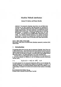
Figure 4 TTT plot for the Golden shiner data.

21 22 23 24 25 26 27 28 29 30 31 32 33 34 35

21

cm); xi4 —depth of the place (in cm); xi5 —abundance index of macro-thin plants (in percentage) and xi6 —transparency of the water (in cm). In many applications there is qualitative information about the hazard shape which can support a specified model. In this context, a device called the total time on test (TTT) plot [Aarset (1987)] is very useful. The TTT plot is obtained by

r

n plotting G(r/n) = [( i=1 Ti:n ) + (n − r)Tr:n ]/( i=1 Ti:n ) for r = 1, . . . , n against r/n, where Ti:n are the order statistics of the sample (i = 1, . . . , n). The TTT plot for Golden shiner data given in Figure 4 has first a convex shape and then a concave shape, thus indicating a bathtub shaped failure rate function. The Golden shiner data have been analyzed by Carrasco, Ortega and Paula (2008) using the LMW regression model. We now reanalyzed these data using the LGMW regression model. First, we consider the equation yi = β0 + β1 xi1 + β2 xi2 + β3 xi3 + β4 xi4 + β5 xi5 + β6 xi6 + σ zi ,

36 37 38 39 40 41 42 43

i = 1, . . . , 106,

22 23 24 25 26 27 28 29 30 31 32 33 34 35

(12)

where the random variable yi has the LGMW distribution. The MLEs (approximate standard errors and p-values in parentheses) are: λˆ = 0.001 (0.003), ϕˆ = 12.855 (20.066), σˆ = 5.086 (2.776), βˆ0 = −1.894 (5.904) (0.748), βˆ1 = 2.197 (0.536) (