The Logic and Expressibility of Simply-typed Call ... - Semantic Scholar

The Logic and Expressibility of Simply-typed Call-by-value and Lazy Languages by

Jon Gary Riecke B.A., Computer Science Williams College (1986) S.M., Electrical Engineering and Computer Science Massachusetts Institute of Technology (1989) Submitted to the Department of Electrical Engineering and Computer Science in partial ful llment of the requirements for the degree of Doctor of Philosophy at the MASSACHUSETTS INSTITUTE OF TECHNOLOGY August 1991

c Massachusetts Institute of Technology 1991 Signature of Author Certi ed by

Accepted by

Department of Electrical Engineering and Computer Science August 26, 1991 Albert R. Meyer Professor of Computer Science and Engineering Thesis Supervisor Campbell L. Searle Chair, Department Committee on Graduate Students

ii

The Logic and Expressibility of Simply-typed Call-by-value and Lazy Languages by Jon Gary Riecke

Submitted to the Department of Electrical Engineering and Computer Science on August 26, 1991, in partial ful llment of the requirements for the degree of Doctor of Philosophy

Abstract

We study the operational, denotational, and axiomatic semantics of lazy and call-by-value functional languages, and use these semantics to build a new expressiveness theory for comparing functional languages. The rst part of the thesis develops the theory of lazy and call-by-value languages separately, following paradigmatic studies of call-by-name functional languages. We rst describe the operational semantics of two simply-typed languages, lazy PCF and call-byvalue PCF. These two languages provide enough intuition to describe general de nitions of denotational models and logics for lazy and call-by-value languages. We prove, via a completeness theorem, that the de nitions of models and logic coincide for both the lazy and call-by-value theories. The second part of the thesis compares the two kinds of languages via translations. Speci cally, we develop the idea of a fully abstract translation and de ne new fully abstract translations from call-by-value PCF to lazy PCF, and vice versa. We then use the ideas to develop an expressiveness theory for languages. The theory shows that call-byvalue PCF and lazy PCF are equally expressive, and another language, call-by-name PCF, is strictly less expressive than either of the other two. Keywords: Operational semantics, denotational semantics, logics of programs, domains, callby-name, call-by-value, lazy languages, adequacy, full abstraction, translations. Thesis Supervisor: Albert R. Meyer Title: Professor of Computer Science and Engineering

iii

iv

v

Acknowledgements I owe a great debt to my advisor, Albert R. Meyer. It was his initial question that set me working on logics and translations for the two languages in this thesis, and his technical help and encouragement along the way were invaluable. My only regret of the time I spent at MIT was not having more time to work on research with Albert. His enthusiasm, philosophical wisdom, and good taste have made a deep impression on me, and I hope, through his example, to develop these qualities in myself. It has also been a pleasure working with two other coauthors: Bard Bloom, once a student at MIT and now a faculty member at Cornell, and Stavros Cosmadakis of IBM Research. I learned a lot from Bard and Stavros, including facts not always connected to computer science! I would also like to thank the members of my thesis committee, David Giord and Rishiyur Nikhil, who provided good comments on a draft of this thesis and during the defense, and Carl Gunter of the University of Pennsylvania, who gave me time to nish the thesis during the rst months of a postdoctoral position. My fellow semantics students (many of whom are now elsewhere) deserve my warmest thanks: Val Breazu-Tannen, Mike Ernst, Lalita Jategaonkar, Trevor Jim, Arthur Lent, Mark Reinhold, Arie Rudich, David Wald, and Paul Wang. They have all, at one time or another, read and critiqued drafts of papers, and helped me formulate my ideas before I started to write. I especially thank Trevor Jim and Mike Ernst for their perceptive comments on the thesis. Others around the Theory of Computation Group at MIT have been great friends and con dants: Arline Benford, Tom and Nicole Cormen, Lance Fortnow, Be Hubbard, David Jones, James Park, Cindy Phillips, Robert Schapire and Roberta Sloan, Eric Schwabe, and Mark and Margaret Tuttle. The softball team also kept me from working too hard. None of this would have been possible without the support of my parents, Gary and Beverly Riecke. They encouraged me to make my own decisions, tempered by Midwestern sensibility, early in my life|even when those decisions entailed going to a strange, liberal arts college far away from home. I feel very lucky to have grown up in a stable household full of common sense and the love of learning. But my deepest thanks go to my wife, Michelle Traina Riecke. She has been the backbone of our nascent family through four and a half years of graduate school, often picking up household

vi duties to allow me time to work. She has been a constant source of encouragement, strength, and most importantly, humor and perspective, in the midst of innumerable problem sets and nerveracking exams. I often doubt that I would have nished without her; and I wish I could give her half the hood I have been working so hard to obtain. I gratefully acknowledge the nancial support provided by the National Science Foundation under the Graduate Fellowship Program and contracts 851190-DCR and 8819761-CCR, and by the Oce of Naval Research under contract N00014-83-K-0125.

vii

Comments on Joint Results Portions of this thesis represent joint work with others. For instance, most of Chapter 3 appeared rst in a joint paper with Stavros S. Cosmadakis and Albert R. Meyer [12], with the exception of Theorem 3.25 which appeared in a joint paper with Bard Bloom [9]. Chapter 4, while my own work unless otherwise speci ed, draws heavily upon the methods of Chapter 3. The results of Chapter 4 appeared in [46]. Chapter 5, in contrast, is almost entirely my own work; the results in this chapter were previously reported in [47].

viii

Contents 1 Introduction

1

1.1 The Theory of Call-by-name PCF : : : : : : : : : : : : : : : : : : : : : : : : : : 2 1.2 Lazy and Call-by-value Languages : : : : : : : : : : : : : : : : : : : : : : : : : : 7 1.3 Outline of the Thesis : : : : : : : : : : : : : : : : : : : : : : : : : : : : : : : : : : 10

2 Syntax and Operational Semantics of PCF 2.1 Simply-typed -calculus : : : : : 2.2 Syntax of PCF : : : : : : : : : : 2.3 Operational Semantics of PCF : 2.3.1 Call-by-name PCF : : : : 2.3.2 Lazy PCF : : : : : : : : : 2.3.3 Call-by-value PCF : : : : 2.4 Comparing the Three Languages

: : : : : : :

: : : : : : :

: : : : : : :

3 Models and Logics of Lazy Languages

: : : : : : :

: : : : : : :

: : : : : : :

: : : : : : :

: : : : : : :

: : : : : : :

: : : : : : :

3.1 Models of Lazy Languages : : : : : : : : : : : : : : 3.1.1 Mathematical preliminaries : : : : : : : : : 3.1.2 Lazy environment models : : : : : : : : : : 3.1.3 Examples of lazy models : : : : : : : : : : : 3.2 Lazy Logic : : : : : : : : : : : : : : : : : : : : : : 3.2.1 Lazy sequent logic : : : : : : : : : : : : : : 3.2.2 Interpretation in at lazy models : : : : : : 3.2.3 Theorems about lazy sequent logic : : : : : 3.3 Completeness for Flat Lazy Models : : : : : : : : : 3.3.1 Henkin completion : : : : : : : : : : : : : : 3.3.2 Constructing lazy models from completions 3.4 Theory of Lazy PCF : : : : : : : : : : : : : : : : : 3.4.1 Review of the essentials of domain theory : 3.4.2 Denotational semantics for lazy PCF : : : : 3.4.3 Relationship to lazy theory : : : : : : : : : 3.4.4 Recursion-free approximations are co-r.e. : 3.5 Conclusion : : : : : : : : : : : : : : : : : : : : : : ix

: : : : : : : : : : : : : : : : : : : : : : : :

: : : : : : : : : : : : : : : : : : : : : : : :

: : : : : : : : : : : : : : : : : : : : : : : :

: : : : : : : : : : : : : : : : : : : : : : : :

: : : : : : : : : : : : : : : : : : : : : : : :

: : : : : : : : : : : : : : : : : : : : : : : :

: : : : : : : : : : : : : : : : : : : : : : : :

: : : : : : : : : : : : : : : : : : : : : : : :

: : : : : : : : : : : : : : : : : : : : : : : :

: : : : : : : : : : : : : : : : : : : : : : : :

: : : : : : : : : : : : : : : : : : : : : : : :

: : : : : : : : : : : : : : : : : : : : : : : :

: : : : : : : : : : : : : : : : : : : : : : : :

: : : : : : : : : : : : : : : : : : : : : : : :

: : : : : : : : : : : : : : : : : : : : : : : :

: : : : : : : : : : : : : : : : : : : : : : : :

: : : : : : : : : : : : : : : : : : : : : : : :

11

11 12 13 14 15 17 17

19

19 19 20 23 24 24 29 29 30 32 36 39 39 40 45 46 49

CONTENTS

x

4 Models and Logics of Call-by-value Languages

4.1 Models of Call-by-value Languages : : : : : : : : : : : : : : 4.1.1 Call-by-value environment models : : : : : : : : : : 4.1.2 Examples of call-by-value models : : : : : : : : : : : 4.2 Call-by-value Logic : : : : : : : : : : : : : : : : : : : : : : : 4.2.1 Interpretation in at call-by-value models : : : : : : 4.2.2 Theorems about call-by-value sequent logic : : : : : 4.3 Completeness for Flat Call-by-value Models : : : : : : : : : 4.3.1 Henkin completion : : : : : : : : : : : : : : : : : : : 4.3.2 Constructing call-by-value models from completions 4.4 Theory of Call-by-value PCF : : : : : : : : : : : : : : : : : 4.4.1 Denotational semantics for call-by-value PCF : : : : 4.4.2 Relationship to call-by-value theory : : : : : : : : : 4.4.3 Recursion-free approximations are co-r.e. : : : : : : 4.5 Conclusion : : : : : : : : : : : : : : : : : : : : : : : : : : :

5 Fully Abstract Translations

5.1 Introduction : : : : : : : : : : : : : : : : : : : : : : : 5.2 Translation from Call-by-Value to Lazy PCF : : : : 5.2.1 The basic translation : : : : : : : : : : : : : : 5.2.2 Adequacy : : : : : : : : : : : : : : : : : : : : 5.2.3 Failure of full abstraction : : : : : : : : : : : 5.2.4 Full abstraction : : : : : : : : : : : : : : : : : 5.3 Call-by-name to Call-by-value PCF : : : : : : : : : : 5.4 Lazy to Call-by-value PCF : : : : : : : : : : : : : : 5.5 Corollaries of Full Abstraction : : : : : : : : : : : : 5.6 Functional Translations : : : : : : : : : : : : : : : : 5.6.1 Godelnumbering translations : : : : : : : : : 5.6.2 De nition of functional translations : : : : : 5.6.3 Distinctions made by functional translations : 5.7 Conclusion : : : : : : : : : : : : : : : : : : : : : : :

: : : : : : : : : : : : : :

: : : : : : : : : : : : : :

: : : : : : : : : : : : : :

: : : : : : : : : : : : : :

: : : : : : : : : : : : : :

: : : : : : : : : : : : : :

: : : : : : : : : : : : : :

: : : : : : : : : : : : : :

: : : : : : : : : : : : : :

: : : : : : : : : : : : : :

: : : : : : : : : : : : : :

: : : : : : : : : : : : : :

: : : : : : : : : : : : : :

: : : : : : : : : : : : : :

: : : : : : : : : : : : : :

: : : : : : : : : : : : : :

: : : : : : : : : : : : : :

: : : : : : : : : : : : : :

: : : : : : : : : : : : : :

: : : : : : : : : : : : : :

: : : : : : : : : : : : : :

: : : : : : : : : : : : : :

: : : : : : : : : : : : : :

: : : : : : : : : : : : : :

: : : : : : : : : : : : : :

: : : : : : : : : : : : : :

: : : : : : : : : : : : : :

: : : : : : : : : : : : : :

6 Conclusion A Sequent Logic

51

51 52 54 56 56 57 57 58 59 62 62 64 65 68

71

71 73 73 74 77 78 86 87 88 89 90 91 98 99

101 105

A.1 Syntax : : : : : : : : : : : : : : : : : : : : : : : : : : : : : : : : : : : : : : : : : : 105 A.2 Basic Axioms and Rules : : : : : : : : : : : : : : : : : : : : : : : : : : : : : : : : 106 A.3 Deduction Theorems : : : : : : : : : : : : : : : : : : : : : : : : : : : : : : : : : : 106

B Proofs of Full Abstraction Theorems

B.1 Translation of Call-by-name to Call-by-value PCF : B.1.1 A fully abstract model for call-by-name PCF B.1.2 Properties of the functions : : : : : : : : : B.1.3 Adequacy : : : : : : : : : : : : : : : : : : : : B.1.4 Translations are in the range of retractions : B.1.5 Surjectivity of the relations R : : : : : : : : :

: : : : : :

: : : : : :

: : : : : :

: : : : : :

: : : : : :

: : : : : :

: : : : : :

: : : : : :

: : : : : :

: : : : : :

: : : : : :

: : : : : :

: : : : : :

: : : : : :

: : : : : :

109

: 109 : 109 : 110 : 112 : 116 : 119

CONTENTS B.1.6 Full abstraction : : : : : : : : : : : : : : : : B.2 Translation of Lazy to Call-by-value PCF : : : : : B.2.1 Properties of the functions : : : : : : : : B.2.2 Adequacy : : : : : : : : : : : : : : : : : : : B.2.3 Translations are in the range of retractions B.2.4 Surjectivity of the relations R : : : : : : : : B.2.5 Full abstraction : : : : : : : : : : : : : : : :

xi

: : : : : : :

: : : : : : :

: : : : : : :

: : : : : : :

: : : : : : :

: : : : : : :

: : : : : : :

: : : : : : :

: : : : : : :

: : : : : : :

: : : : : : :

: : : : : : :

: : : : : : :

: : : : : : :

: : : : : : :

: : : : : : :

: 122 : 123 : 123 : 124 : 129 : 132 : 135

xii

CONTENTS

Chapter 1

Introduction When checking the correctness of a program, programmers use many dierent styles of informal reasoning. First, some informal knowledge of the interpreter may guide the programmer: a while statement, for instance, causes the interpreter to loop over a section of code \while" a certain condition is satis ed. Second, mathematical intuitions about the constructs of the language may provide insight. For example, the + operator satis es many principles governing actual addition. Third, encapsulated principles gained from experience may be employed. These vague ideas have been formalized into three styles of assigning meaning to programs. 1. Operational Semantics: Specifying a complete de nition of the language interpreter, together with a notion of what is \observable" about the interpreter. 2. Denotational Semantics: Formalizing the language constructs into more mathematicallooking entities, where the meaning of code is determined by the meaning of its parts. For example, in a functional language, we might choose to denote user-de ned functions by true mathematical functions. 3. Axiomatic Semantics: Developing logical principles for proving facts about code. Hoare logics [24] and pure -calculus equational reasoning [4] fall into this category. None of these three forms of semantics can convincingly be claimed superior to the others; on an informal level, programmers seem to use them all. It is therefore worthwhile to develop all three semantics. 1

2

CHAPTER 1. INTRODUCTION

This thesis studies the operational, denotational, and axiomatic semantics of lazy and callby-value functional languages. Much of the thesis will focus on two simple languages, lazy and call-by-value PCF (Programming language for Computable Functions), which are languages based on the simply-typed -calculus that include basic arithmetic, conditionals, and recursion [41, 51]. These languages are important precisely because they are simpli ed versions of some of the more familiar, widely-used functional languages, e.g., Scheme [1, 44], LISP [65], ML [28, 29], and Haskell [23]. Ultimately, by studying the semantics of PCF, we hope to gain insight into the semantics of more complicated languages. The thesis has two main parts. The rst part studies the operational, denotational, and axiomatic semantics of lazy and call-by-value PCF in isolation, and proves theorems that show the close connections between the three semantics. The second part describes the relationships between lazy and call-by-value PCF using translations. We nd that lazy PCF and call-byvalue PCF can be translated into one another in a way that preserves the meaning of code. The translations are entirely mechanical, and do not rely on the inherent computing power of the two languages. The existence of meaning-preserving translations has important consequences. First, if a meaning-preserving translation is used as the basis of a compiler, optimizations carried out on either source or target programs can be shown to be valid. Other semantical properties carry over as well. Second, translations have a close connection to expressiveness; intuitively, language A is no more expressive than language B if one can mechanically translate programs written in language A into language B. We develop this idea to build a rudimentary but new expressiveness theory based on translations, which we then use to compare the expressiveness of call-by-name, lazy, and call-by-value PCF.

1.1 The Theory of Call-by-name PCF The studies of call-by-name PCF and the simply-typed -calculus [41, 43, 49, 63] provide a paradigm for developing the semantics of lazy and call-by-value languages. The connections between operational, denotational, and axiomatic semantics for call-by-name PCF are the ones we will seek for lazy and call-by-value languages. Also, many, though not all, of the proof techniques from the call-by-name case will carry over to the lazy and call-by-value cases.

1.1. THE THEORY OF CALL-BY-NAME PCF

3

Operational semantics is the most familiar place to begin. In general, designing an operational semantics involves building an interpreter and deciding which properties of the interpreter are observable. For functional languages, we typically choose the observations to be the \printable values" of computations, e.g., numerals, booleans, or lists of printable values [7, 27, 41], since these observations have the most to do with the correctness of code. In the case of call-byname PCF, the observations are the ground constants, i.e., the numerals.1 Thus, for example, the PCF terms (succ 3) and (pred 5) both produce the observable output 4. Of course, these observations tell us nothing about the behavior of functional pieces of code. In call-by-name PCF, for example, functions produce no observable behavior. Nevertheless, many functional terms may be distinguished by placing them in a context|a term with one or more \holes." For example, the context C [] = ([] 1) distinguishes (x succ x) from (x pred x), since C [x succ x] reduces to 2 whereas C [x pred x] reduces to 0.

De nition 1.1 Two terms M and N are observationally distinguishable with respect to some collection O of observations in some language L if for some L-context C [], C [M ] and C [N ] yield dierent observable behavior (according to O). The negation of observational distinguishability is what we will mean by code equivalence.

De nition 1.2 Two terms M and N are observationally congruent with respect to some collection O of observations in some language L (written M OL N ) i they are not observationally distinguishable with respect to O. Observational congruence in call-by-name PCF is written M name N . Observational congruence gives precise meaning to the programmer's intuition of equivalent pieces of code. For example, when observing the nal outputs of programs and not their time or space usage, mergesort and quicksort are equivalent in most languages since they produce identical behavior in all contexts. Observational congruence can also be used in proving that code meets a speci cation. To check the correctness of a sort routine S , for instance, we could write the routine D that tries all permutations of a list until it reaches the sorted version, and then show that this \dumb" sort routine D and the original routine S are observationally 1

The versions of PCF considered here do not have booleans.


4

congruent when observing nal answers. Finally, observational congruence captures the notion of correct optimizations: replacing M by a faster but observationally congruent term N will not change the nal answer of the program. Some examples of observational congruences in call-by-name PCF are 1. (succ 3) name 4: Both terms produce the same numeral and from this, one may show that the terms are observationally congruent. In general, two closed, call-by-name PCF terms of type \integer" (henceforth abbreviated ) are observationally congruent i they either both reduce to the same numeral, or both diverge. 2. Two de nitions of addition: Consider the following recursive speci cations of functions over pairs of natural numbers. 8 > : f1 (x ? 1; y ) + 1 otherwise 8 > : f2 (x ? 1; y + 1) otherwise The addition function satis es the equations for f1 and f2 . Both recursive speci cations may be translated into call-by-name PCF by the terms

F1 = f x y cond x y (succ (f (pred x) y)) F2 = f x y cond x y (f (pred x) (succ y))

Here, f M is a recursive declaration, where a recursive call to f may appear in the body M . The cond operator of call-by-name PCF is a conditional: if the rst argument is 0, cond returns its second argument, and if the rst argument is greater than 0, cond returns its third argument. The reader may recognize that both F1 and F2 compute the addition function, but in slightly dierent ways: F2 is tail-recursive and hence may be faster than F1 depending on the implementation of the interpreter [1]. Nevertheless, either may be used in a context with the same results, i.e., F1 name F2 .

3. The previous example may be generalized to a broader principle: observational congruence in call-by-name PCF is extensional, viz., functional terms are congruent i they are congruent when applied [7, 8, 27, 41]. Formally,

1.1. THE THEORY OF CALL-BY-NAME PCF

5

Proposition 1.3 Let M and N be any terms of type ( ! ). Then M name N i for all P of type , (M P ) name (N P ). This implies that

(x M x) name M

(where x is not free in M ) for any term M of functional type. Intuitively, a function M cannot be distinguished from a function that takes an argument x and immediately applies M to that argument. 4. The \functional" behavior of -abstractions is often characterized by the observational congruence ((x M ) N ) name M [x := N ]

where M [x := N ] denotes substitution of N for x in M , with the necessary renaming of bound variables to avoid capture of free variables [4]. Each of the above congruences can be justi ed informally, but how can one formally verify these congruences? Formal proofs from the operational semantics alone can be tedious and long; the skeptical reader may wish to attempt a proof of F1 name F2 using the interpreter in Chapter 2. Some general lemmas, such as operational extensionality given in Proposition 1.3, can be used to simplify the proof, but collecting these facts is dicult without further insight. Denotational semantics can provide this insight. Instead of reasoning with the interpreter, we translate terms into some mathematical \meaning" in the denotational model. A well-chosen denotational semantics, suciently divorced from the details of the interpreter, can be used to verify observational congruences more easily. Standard mathematical concepts can be used to assign denotational semantics to call-byname languages. Points 3 and 4 above show that functionally-typed terms indeed have certain logical properties like those of mathematical functions. It is therefore not surprising that most denotational models for call-by-name languages are constructed out of function spaces. For callby-name PCF, the most familiar denotational semantics is the model N built out of continuous functions over certain partially-ordered sets known as Scott domains [22, 52]. (This model is de ned precisely in Appendix B, page 109.) These domains provide an interpretation for recursion and the other constructs of call-by-name PCF.


6

For denotational reasoning to be sound, there must be some connection between denotational equivalence and the operational semantics. The minimum desired property is adequacy, which states that the denotational model faithfully predicts the observable behavior of code. For callby-name PCF,

Theorem 1.4 The model N is adequate. That is, for any closed PCF term M of type , N [ M ] = k i M evaluates to the numeral denoted by k. There are a number of adequate semantics for call-by-name PCF [41]. The deeper connection between operational and denotational semantics is called full abstraction [26, 27, 41, 66].

De nition 1.5 A denotational semantics [ ] is equationally fully abstract if for any terms M and N , [ M ] = [ N ] i M OL N . It turns out that N is equationally fully abstract for call-by-name PCF.2

Theorem 1.6 (Plotkin,Sazonov) For any call-by-name PCF terms M and N , N [ M ] = N [ N ] () M name N: The full abstraction theorem allows us to substitute denotational for operational reasoning, usually with great bene t: observational congruences are often easier to prove denotationally than operationally. For instance, it is not hard to prove that the terms F1 and F2 are both denoted by the addition function in the model N . Since their meanings are equivalent in a fully abstract model, the terms are observationally congruent. More general congruences are also easy to verify. For example, the familiar equational axioms ( ) ( )

((x M ) N ) = M [x := N ] (x M x) = M; where x not free in M

hold in the model and hence by full abstraction are valid when we interpret = as the observational congruence relation name . The familiar congruence rules (substitution of equals for equals, and the axioms and rules for equivalence relations) are also easy to check using the model N . 2 The expert reader may recall that call-by-name PCF must have certain \parallel" operators for this full abstraction theorem to hold. The versions of PCF studied here will always include these parallel operators.

1.2. LAZY AND CALL-BY-VALUE LANGUAGES

7

Collecting principles such as ( ) and ( ) is a way to build the third form of semantics, an axiomatic semantics. In general, an axiomatic semantics is a formal system for proving facts about code. The axiomatic semantics for call-by-name PCF proves equations between terms. Other styles, such as Hoare logics [24], prove rst-order statements about code. Just as for denotational semantics, there must be some connection between the operational and axiomatic semantics. A good axiomatic semantics must be sound, i.e., everything provable is true. It should also prove as many facts about code as possible; if it proves all true facts about code, the system is called complete. In the case of call-by-name PCF, the equations ( ) and ( ) are sound when we interpret = as name . Other equations, e.g., F1 = F2 , are sound but not provable alone from ( ), ( ), and the congruence rules. We might try to capture all observational congruences in a complete proof system for call-by-name PCF, but this is impossible in an r.e. proof system [51]. Nevertheless, we can obtain a connection between -equality and denotational semantics: -equality axiomatizes precisely those equations that hold in all denotational models of call-byname languages. Friedman proves this fact by de ning the notion of a call-by-name denotational model based on function spaces between sets, and showing that -equality captures those equations that hold in all models [17]. Since N ts this de nition of a model, the axioms ( ) and ( ) provide a good basis for reasoning about call-by-name PCF. We may then extend the proof system with axioms for other constructs (successor and predecessor, numerals, conditionals), and add rules for reasoning about recursion (e.g., Scott induction [20, 51]).

1.2 Lazy and Call-by-value Languages Call-by-name PCF is admittedly a toy language, but we expect its semantics to be a re ection of the semantics of real functional languages. Unfortunately, this is only true up to a certain point: most real functional languages either pass arguments by-name but have more possible observations at functional type, or pass arguments by-value instead of by-name. The semantical theory of call-by-name languages is inapplicable to both situations. Consider, for instance, the operational semantics of call-by-name languages such as Haskell [23]. Printable values (e.g., numerals) are observable in Haskell, just as in call-by-name PCF; but there is another computational behavior that is observable, namely termination of evaluation. A Haskell interpreter


8

halts not only on printable values, but also halts and prints a prompt at -abstractions, viz., when it can build a closure. A language will be called lazy if one can observe termination at functional type.3 The call-by-name theory is not suited to proving facts about lazy languages. One example in a -calculus-based language clari es this point: let be a divergent term of type ( ! ), and let M1 = (x x) and M2 = . Under most interpreters for call-by-name languages (cf. [9, 21, 41]), the evaluation of M1 converges and the evaluation of M2 diverges. The axiom ( ), however, states that the terms M1 and M2 are equivalent. Therefore, ( ) is not sound when observing termination. The example of M1 and M2 also shows that N is not even adequate for observing termination, since there is no denotational distinction made between the observably distinct terms M1 and M2 . More obvious obstacles in applying the theory of call-by-name PCF arise when we consider the parameter-passing mechanism. Languages such as Scheme [1, 44], LISP [65], and ML [28, 29] pass arguments by-value instead of by-name, i.e., arguments are reduced to values (constants or -abstractions) before substitution in function bodies. Call-by-value interpreters are generally easier and more ecient to implement than call-by-name interpreters; for this reason, call-byvalue is the most widely-used parameter-passing mechanism in functional languages. The call-by-name theory is unsound for reasoning in call-by-value languages. For instance, let be a divergent term of type ( ! ). Then the terms ((x! 3) ) and 3 are equivalent via ( ) but are not observationally congruent in the call-by-value version of PCF: the rst diverges whereas the second halts. This example also points to denotational problems; the model N fails to be adequate for call-by-value PCF. These examples show that lazy and call-by-value languages|the most widely used functional languages|require new denotational and axiomatic principles. This fact is somewhat surprising, for it shows a large gap between the theoretical community (which has been largely content to study call-by-name languages) and the practical community. Good denotational models for lazy and call-by-value languages are not dicult to de ne. Like the model N , models for these languages can be built using partially-ordered sets and

3 The word \lazy" here does not refer to lazy lists. This is somewhat confusing terminology, but it maintains a link with the earlier work of Abramsky [2, 3] and Ong [38, 39].

1.2. LAZY AND CALL-BY-VALUE LANGUAGES

9

function spaces [9, 11, 57, 58], although the meanings of functionally-typed terms are not quite functions, since the operational semantics of lazy and call-by-value languages do not obey the extensionality property. Full de nitions appear in Chapters 3 and 4. In contrast, logical principles dier greatly from the call-by-name case. It is not hard to gather some sound logical principles together. For instance, the restricted version of the ( ) equation ( v )

((x M ) V ) = M [x := V ]; for V a value

is sound for call-by-value [40]. A similarly-restricted version of ( ) is sound for both lazy and call-by-value languages. But it seems dicult to restrict the ( ) and ( ) axioms to cover all equations that hold in lazy or call-by-value languages. As we shall point out in Chapters 3 and 4, no equational axiom system can be complete for proving those equivalences that hold in all simply-typed lazy or call-by-value languages. It turns out that reasoning by cases is needed in both situations. The logics of Chapters 3 and 4 capture reasoning by cases using sequents (de ned more formally later). This is not a new idea; in [34], Moggi develops higherorder sequent logics for call-by-value languages, and in [39], Ong develops a natural deduction logic, a slightly restricted form of a sequent logic, for lazy languages. We shall point out the dierences between our logics and theirs in Chapters 3 and 4. Reasoning about lazy and call-by-value languages also seems to require proving approximations rather than equations. In addition to obvious connections to the partial order structure of denotational models of lazy and call-by-value languages, approximations have a purely operational characterization:

De nition 1.7 A term M observationally approximates a term N with respect to L and O, written M vOL N , i, for any L context C [], if C [M ] yields an observation in O, then C [N ] yields the same observation.

Of course, M OL N i M vOL N and N vOL M . Approximations and the predicates of convergence and divergence will form the basis of the sequent logics for lazy and call-by-value languages.

10


1.3 Outline of the Thesis Chapter 2 de nes operational semantics of the lazy and call-by-value versions of PCF. Each language is based on call-by-name PCF, whose de nition is also included in Chapter 2. We de ne interpreters for the languages and also de ne precisely the observational approximation relations. Chapters 3 and 4 develop denotational and axiomatic semantics for lazy and call-by-value languages. De nitions of denotational models and sequent logics for these classes of languages appear in these chapters, along with completeness theorems that demonstrate the match between the class of models and the logic. Chapters 3 and 4 also consider the particular denotational and axiomatic semantics of lazy PCF and call-by-value PCF, describing fully abstract models and their relationship to the axiomatic semantics. Despite the major dierences between call-by-name, call-by-value, and lazy PCF, there are quite a few similarities. Chapter 5 exploits these similarities, showing how to translate languages into others. The translations will yield corollaries on the complexity of certain decision problems in the denotational and operational semantics. We also develop a notion of \functional translation" that generalizes our translation technique, and use it as the basis of an expressiveness theory. We are able to show that call-by-name PCF is strictly less expressive than either lazy or call-by-value PCF, and that lazy and call-by-value PCF are equally expressive. Chapter 6 concludes the thesis with a discussion of open problems.

Chapter 2

Syntax and Operational Semantics of PCF This chapter brie y de nes the syntax and operational semantics of three versions of PCF, callby-name, call-by-value, and lazy PCF. PCF is a higher-order functional language with basic arithmetic operators, conditionals, and recursion. The syntax thus contains the core of many functional languages, but is complex enough to bring out many of the subtle problems arising in assigning semantics to functional languages. The main dierences between the three languages appear in their operational semantics, and in particular, in the parameter-passing mechanisms employed. These dierences will be important in the following chapters.

2.1 Simply-typed -calculus The simply-typed -calculus is the core of PCF. Each term in the simply-typed -calculus comes with a simple type. Simple types are de ned inductively to be the base type , usually taken to be the type of natural numbers, and ( ! ), the type of functions from to , where and themselves are types.1 We often drop parentheses from types with the understanding that ! associates to the right: for example, ( ! ( ! )) is abbreviated ( ! ! ). Thus, any simple type can be written in the form (1 ! 2 ! : : :n ! ) for some n 0. 1 We use only one base type for simplicity; other formulations of the simply-typed -calculus include more than one base type, e.g., [41].

11

CHAPTER 2. SYNTAX AND OPERATIONAL SEMANTICS OF PCF

12

xi : , where i 2 N Constants -abstraction (x MM) :: ( ! ) Application i

Variables

c : , if c 2 M : ( ! ) N : (M N ) :

Table 2.1: Syntactic formation rules for the simply-typed -calculus. Terms in the simply-typed -calculus are given over a set of typed constants called a signature; for simplicity, signatures are always assumed to be countable. The simply-typed -calculus over is the least set closed under the operations of Table 2.1. The set of pure terms is the set of simply-typed -calculus terms over the empty signature. A simply-typed language is any countable set of terms over a signature , where every term is assigned a simple type, and which is closed under the operations of variables, constants, -abstraction, and application. A simply-typed language may therefore have more means of constructing terms than just -abstraction and application. An extension L0 to a simply-typed language L is a simply-typed language in which L L0; extensions will often be constructed by adding more constants and closing up under -abstraction and application. We adopt many of the standard notational conventions of the -calculus [4]. For instance, terms are denoted by the letters M , N , P , Q, S , and T . Parentheses may be dropped from applications under the assumption that application associates to the left, i.e., (M N P ) is short for ((M N ) P ). We will also drop types from variables whenever the types are unimportant or can be deduced from the context, and use the letters u, v , w, x, y , and z to denote variables. The usual de nitions of free and bound variables apply here, and terms are identi ed up to renaming of bound variables [4]. Finally, syntactic substitution is written M [x := N ], where the substitution renames bound variables to avoid capturing the free variables of N [4].

2.2 Syntax of PCF PCF (Programming language for Computable Functions) is a simply-typed language which has some simple constructs for computing with integers. The set of PCF-terms is the least set closed under the operations of variables, -abstraction, application, and the formation rules of

2.3. OPERATIONAL SEMANTICS OF PCF

Numerals Successor Conditional

0; 1; 2; : : : :

M : (succ M ) : M : N : P : (cond M N P ) :

13

Recursion Predecessor Parallel conditional

M : x M : M : (pred M ) : M : N : P : (pcond M N P ) :

Table 2.2: Additional syntactic formation rules for PCF. Table 2.2.2 A term is a value if it is a numeral or -abstraction; values are denoted by V . The sequential conditional (cond M N P ) reduces its rst argument, returning the value of the second if the rst halts at 0 and the value of the third if the rst halts at a numeral greater than 0. The parallel conditional (pcond M N P ), where M , N , and P have type , diers from (cond M N P ) operationally in one respect: if N and P reduce to the same numeral, (pcond M N P ) reduces to that numeral even if M diverges. As we shall brie y argue in Chapters 3 and 4, pcond is necessary for making the standard denotational models fully abstract. PCF is the syntax of call-by-name and call-by-value PCF. For lazy PCF, we add the rule Convergence-testing

M :

N : (conv M N ) :

and call the resultant set of terms LPCF. Informally, (conv M N ) returns the value of N if the interpretation of M halts, and otherwise diverges.

2.3 Operational Semantics of PCF The operational semantics of PCF can be de ned by a deductive semantics.3 A deductive semantics de nes a binary relation + on terms by rules based on the structure of terms; we There are alternative ways of building a syntax of PCF. Most notably, the syntax can be de ned using constants instead of term constructors [41]. Using constants for conditionals, however, leads to a rather arcane operational semantics of call-by-value PCF (cf. [59]). 3 This form of semantics has been given the unfortunate title \natural semantics" by Gilles Kahn and others; it has also been called an \observation calculus" by Bloom [8]. We call this form of semantics a \deductive semantics" to emphasize the resemblance of the interpretation of terms to proof trees. 2


14

V + V; V a value M +n

(succ M ) + (n + 1) M + (n + 1) (pred M ) + n M +0 (pred M ) + 0 M [x := x M ] + V (x M ) + V

M +0 N +V (cond M N P ) + V M + (n + 1) P + V (cond M N P ) + V M +0 N +k (pcond M N P ) + k M + (n + 1) P + k (pcond M N P ) + k N +k P +k (pcond M N P ) + k

Table 2.3: Deductive semantics rules for applying constants and reducing conditionals. write M + V (read \M halts at value V ") when there is a proof tree with result M + V , whose nodes are instances of the rules de ning the relation +. It is important to understand the substantial dierence between deductive semantics and rewrite or \structured operational semantics" [4, 42]. In deductive semantics, terms are written to values in one big step, whereas in rewrite semantics, the single-step relation may need to be used multiple times in order to rewrite a term to a value. Each language has its own + relation, called +n , +v , and +l for call-by-name, call-by-value, and lazy PCF respectively. The rules de ning these relations include the rules of Table 2.3.4 Rules speci c to the three languages appear in Table 2.4.

2.3.1 Call-by-name PCF The call-by-name interpreter requires one more rule beyond those appearing in Table 2.3. This is the rule for evaluating applications of -abstractions to arguments, where the arguments are passed call-by-name, i.e., without evaluation, which appears in Table 2.4. For call-by-name PCF, we observe only numerals [41], and hence the observational approximation relation is The expert reader may recall that Plotkin's interpreter for call-by-name PCF diverges on (pred 0) [41], whereas our interpreter returns 0. This is a minor design change that makes the denotational semantics of the three languages easier to use. 4

2.3. OPERATIONAL SEMANTICS OF PCF

15

M +n x M 0 M 0[x := N ] +n V (M N ) +n V

Call-by-name

M +l x M 0 M 0 [x := N ] +l V (M N ) +l V

Lazy

M +v x M 0

Call-by-value

M +l V 0 N +l V (conv M N ) +l V

N +v V 0 M 0 [x := V 0 ] +n V (M N ) +v V

Table 2.4: Deductive semantics rules speci c to the three languages.

De nition 2.1 M vname N if for any PCF-context C [], C [M ] +n k implies C [N ] +n k. For example, let = f ! f ; then (x x) vname . The examples of Chapter 1 are also examples of call-by-name observational approximations.

2.3.2 Lazy PCF Like the call-by-name interpreter, the lazy interpreter also passes arguments by-name. Nevertheless, there is one signi cant dierence between the two languages: lazy PCF includes extra terms for convergence-testing. These extra terms are interpreted by the rule given in Table 2.4. In lazy PCF we observe numerals, so

De nition 2.2 M vlazy N if for any LPCF-context C [], C [M ] +l k implies C [N ] +l k. Some examples of lazy approximations and congruences are 1. (succ 3) lazy 4: As with call-by-name PCF, two closed terms of type are lazy congruent i both produce the same numeral, or both diverge. 2. vlazy M : In the empty context, a looping term never produces any observable behavior. Suppose, however, that C [ ] produces a numeral output. Then the lazy interpreter never gets stuck reducing , and thus never evaluates the term in the \hole." Hence, for any term M , the term C [M ] must produce the same observation as C [ ].


16

3. (x P ) 6vlazy : Note that the left side converges whereas the right side diverges. The context (conv [] 0) distinguishes these two terms, since (conv (x P ) 0) +l 0 but (conv 0) *l.

4. M vlazy (x M x), where M is closed: If M diverges, the fact that M vlazy (x M x) follows from the previous example. If M converges, these terms are actually observationally congruent: the only way to distinguish convergent terms of higher type is to apply them to other terms, and M and (x M x) have the same behavior when applied. Note, however, that (x M x) vlazy M does not hold in general, since M may diverge whereas (x M x) always converges.

5. ((x M ) N ) lazy M [x := N ]: As in the call-by-name PCF, the operational version of the ( ) axiom holds by the fact that parameters are passed by-name.

These informal arguments can be turned into operational proofs, or the approximations can be veri ed in the fully abstract model of Chapter 3. It is important to notice that one may observe termination and obtain the same observational approximation relation. Suppose, for example, M 6vlazy N by the context C [] and C [M ] +l m and C [N ] +l n with m < n. Then the context D[] = (cond (predm C []) 0 ), where (predm P ) = (|pred (pred {z : : : (pred} P ))) m times forces D[M ] to converge but D[N ] to diverge. Both numeral and termination observations will be important in the de nitions of Chapter 5, even though only one kind of observation is essential in de ning the lazy observational congruence relation. In contrast, observing termination in call-by-name PCF yields a dierent observational approximation relation than vname . For instance, (x x) name where is a divergent term of functional type, but in the empty context, the (x x) +n but *n . As an intermediate problem, one could study the semantics (operational, denotational, and axiomatic) of observing termination in call-by-name PCF (which lacks convergence-testing). We leave this study open, mainly because convergence-testing is necessary in order to obtain a full abstraction theorem for the most straightforward denotational models (see Chapter 3).

2.4. COMPARING THE THREE LANGUAGES

17

2.3.3 Call-by-value PCF The call-by-value version of PCF diers little from call-by-name or lazy PCF. The main difference between the languages arises in the parameter-passing mechanism implemented by the interpreter: in call-by-value PCF, all arguments are reduced to values before being substituted for formal parameters. The formal rule appears in Table 2.4. The observations of call-byvalue PCF are numerals, so as before,

De nition 2.3 M vval N if for any PCF-context C [], C [M ] +v k implies C [N ] +v k. Some examples of call-by-value congruences are 1. (cond 3 2 1) val 1: This observational congruence follows from the fact that the left hand side reduces to the right hand side. As with call-by-name and lazy PCF, two closed terms of type are call-by-value observationally congruent i both produce the same numeral, or both diverge. 2. (x x) val (x y x y ): Suppose both terms are placed in a context C []. If x is ever instantiated by a term N during the evaluation of C [x x], that term N must be a value. Since values always halt, N val (y N y ). The observational congruence now follows from this fact.

One may also verify these observational congruences using the fully abstract model of Chapter 4.

2.4 Comparing the Three Languages At the level of interpreters, the three languages de ned above are all quite similar. Lazy PCF is merely an extension of call-by-name PCF to include convergence-testing; likewise, the call-byvalue PCF interpreter is a restricted version of the call-by-name PCF interpreter. But on the level of observational approximations, the similarities seem to disappear: for any two of the three languages, there is an observational congruence that holds in one that does not hold in the other. For example, ((x 0) (f f )) name 0 but ((x 0) (f f )) 6val 0. Nevertheless, there are similarities between the three languages, even at the level of observational approximation. This fact will become somewhat clearer in the next two chapters, when we develop the denotational

18


and axiomatic theory of lazy and call-by-value languages, but will only become truly clear in Chapter 5 when we build translations among the three languages.

Chapter 3

Models and Logics of Lazy Languages In order to reason about programs, it is useful to have denotational and axiomatic means to supplement operational reasoning. This chapter develops the denotational and axiomatic semantics of lazy languages. First, we de ne the notion of a at lazy model and a corresponding logic for reasoning about lazy models. We then prove a completeness theorem: every statement valid in all at lazy models is provable in the logic, and vice versa. We next consider the particular case of lazy PCF, de ning a at lazy model that is adequate and inequationally fully abstract for lazy PCF. For a signi cant subset of LPCF-terms, we also show that the set of approximations not valid in the fully abstract model is r.e.

3.1 Models of Lazy Languages 3.1.1 Mathematical preliminaries We brie y review some of the technical de nitions associated with partially-ordered sets (posets) and domain theory. The informed reader may care to skim this section and refer to it only when necessary. A more complete explanation of the de nitions may be found in [22, 52]. A relation vD on a set D is a partial order if it is re exive (d v d), antisymmetric (d v e and e v d implies d = e) and transitive (d v e and e v f implies d v f ). A partially ordered 19

CHAPTER 3. MODELS AND LOGICS OF LAZY LANGUAGES

20

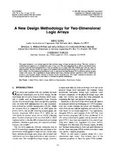
Figure 3-1: A pointed partial order and its lifted version. The arrows show the collapse of the lifted space via drop.

set (D; vD) is a set of elements D with a partial order vD on those elements. We often write D for the partial order and drop the subscript on vD when no confusion can arise. A poset D is pointed if it has a least element, i.e., there exists d 2 D such that for all e 2 D, d v e. A poset D is discretely-ordered if d vD e implies d = e.

One way of building new posets from others is by lifting. If D is a poset, D? denotes the poset comprising D and a new element ?, with ? ordered below every element of D. Furthermore, if D is pointed, there are well-de ned injections lift : D ! D? and projections drop : D? ! D. Figure 3-1 depicts a pointed poset, its lifted version, and the action of the projection function drop. Note that drop(lift(d)) = d and lift(d) 6= ? for all d 2 D. Function spaces over posets will be a key ingredient in the de nitions of models. Let D and E be posets. A function f from D to E is monotone if it preserves the partial order structure of D, viz., d vD e implies that f (d) vE f (e). The monotone function space [D !m E ] is a poset composed of all total monotone functions from D to E , ordered pointwise, i.e.,

f v[D!m E] g () 8d 2 D:f (d) vE g(d): If E is a pointed poset, the monotone function space [D !m E ] is also pointed; the minimum element in this space is the function that maps every d 2 D to the minimum element of E .

3.1.2 Lazy environment models Models of call-by-name languages are usually built out of function spaces. For lazy languages, though, certain principles from the usual mathematical theory of functions are not operationally sound. Extensionality is the key principle that fails. For example, the lazy PCF terms M1 =

and M2 = (x x), where is a divergent term of type ( ! ), are extensionally the same|

3.1. MODELS OF LAZY LANGUAGES

21

both diverge when applied. Nevertheless, M1 diverges whereas M2 converges, so the two terms are not lazy observationally congruent. Extensionality fails only on this kind of example. In lazy PCF, two closed terms M and N of functional type are observationally congruent i both diverge or both converge, and for all closed terms P , (M P ) and (N P ) are observationally congruent. This property may be extended to observational approximation in the obvious way:

Proposition 3.1 Let M; N be closed LPCF-terms of type ( ! ). Then M vlazy N i 1. (M +l ) implies (N +l ); and 2. For any closed LPCF-term P of type , (M P ) vlazy (N P ).

We call this property lazy extensionality (called \conditional weak extensionality" in other studies [3, 38, 39]); it is a key principle of lazy functional languages. Proposition 3.1 is essentially a lazy version of the Context Lemma [27] or operational extensionality [8], and can be proven directly in a similar way or can easily be seen to be a consequence of a full abstraction theorem for the model L de ned below. We omit the proof of the proposition. Two other operational facts, which we also state without proof, provide guidance in building the de nition of \lazy model." The rst of these facts concerns the behavior of functional terms when applied to arguments. Consider, for instance, a divergent term , and suppose (M ) converges under the lazy PCF interpreter. Then (M N ) must also converge for any other term N of the appropriate type: if (M N ) diverges for some term N 6lazy , then M would be able to solve the halting problem. More generally,

Proposition 3.2 Suppose M is a term of type ( ! ), and P vlazy Q where P and Q are terms of type . Then (M P ) vlazy (M Q). In other words, the application of a lazy PCF term is monotone with respect to vlazy . We therefore take monotonicity as a key property of lazy languages. The second fact concerns the behavior of base type terms.

Proposition 3.3 Suppose M and N are closed LPCF-terms of type . If M converges and M vlazy N , then M lazy N .

22


This property is called atness, since for terms of type , there are no proper vlazy -chains of length more than two. Flatness is a key property of the most familiar base types (e.g., numerals, booleans, reals), but there are natural examples of lazy languages with non- at base types. We leave further discussion of this issue to Chapter 6. These properties are essential in de ning the notion of a lazy model. Lazy models have two components. The rst component is a lazy type frame, which is built from a collection of posets indexed by types. The elements of these posets will give meaning to terms, and will satisfy the lazy extensionality, monotonicity, and atness properties. Two other pieces are needed to ensure that these three properties are satis ed: a collection of predicates for interpreting divergence, and an abstract application operator for \applying" elements in the poset assigned to type ( ! ) to elements in the poset assigned to type .

De nition 3.4 A lazy type frame is a tuple (fD : a typeg; f" : a typeg; fA; : ; typesg); where each D is a poset, " D is a set with at most one element, and A; : D ! D ! D . We write d " whenever d 2 ", and d # whenever d 62 ". The components of a lazy type frame must also obey the following properties: 1. If d ", then d v e for all e 2 D ; 2. If d ", then A(d; e) "; and 3. f vD ! g i (a) f # implies g #, and (b) for all d vD e, A(f; d) vD A(g; e). A at lazy type frame is a lazy type frame (fD g; f" g; fA; g) in which D is either discretely-ordered or D = E? where E is discretely-ordered.1 Second, there is a meaning function [ ] that assigns elements of a lazy type frame to terms. Free variables are assigned meanings using environments.

De nition 3.5 Let D be a lazy type frame. A D-environment is a map from variables to elements of D that respects types, i.e., (x ) 2 D for all x . 1 This is a slightly nonstandard usage of the term \ at"; usually, a poset D is said to be at if D = E? for some discretely-ordered E . The generalized de nition allows a slightly expanded class of models.

3.1. MODELS OF LAZY LANGUAGES

23

We use the notation [x 7! d] for a new environment such that ([x 7! d])(y ) = (y ) if y 6= x and d otherwise.

De nition 3.6 Let L be a simply-typed language. A lazy environment model over L is a lazy type frame D with a meaning function [ ] that satis es the equations [ x ] = (x ) [ (M N )]] = A([[M ] ; [ N ] ) [ x M ] = f; where f # and A(f; d) = [ M ] [x 7! d]

and where [ M ] 2 D for any L-term M of type .2 A at lazy environment model is a lazy environment model built from a at lazy type frame. By the de nition of lazy type frame, the meaning of pure simply-typed terms is uniquely determined. Note that the meaning of a closed term is independent of the choice of environment, i.e., if M is closed, then [ M ] = [ M ] 0 for any environments and 0. Therefore, for brevity, the environment will often be dropped when describing the meaning of a closed term. The de nition of lazy model is quite close to the de nition of untyped lazy model given originally by Abramsky [2, 3] and further examined by Ong [39]. Almost all of the ingredients| the de nition of an abstract divergence set, the requirement of lazy extensionality|are present in these de nitions. The only criterion missing is atness, which is not needed for models of untyped lazy languages without constants.

3.1.3 Examples of lazy models There are a number of natural examples of lazy models. For instance, one model can be built out of lifted, monotone functions as follows. If D is any poset, then the full monotonic lazy hierarchy over the poset D, de ned

F = D F ! = [F !m F ]? " = f?g A; (f; d) = drop(f )(d) 2 This clause is necessary in case the language L includes constants or term constructors, e.g., our formulation of PCF.

24


is a lazy model for the pure simply-typed language. The equations in the de nition of model uniquely determine a meaning function F [ ] such that F [ M ] 2 F for any M of type . If D is either discretely-ordered or D = E? for some discretely-ordered E , then the model is a

at lazy model. Other examples of at lazy models include the classical type hierarchy of total functions over a set B , de ned

S = B S ! = [S ! S ] " = ; A; (f; d) = f (d) where [S ! S ] is the set of total functions from S to S . Indeed, any model of the call-byname -calculus (cf. [17, 21]) is a at lazy model.

3.2 Lazy Logic 3.2.1 Lazy sequent logic Axiomatizing the theory of at lazy models cannot be done without some form of reasoning by cases; reasoning using inequational logic alone is necessarily incomplete. For example,

Proposition 3.7 Let A be the set of equations and approximations valid in all at lazy models over the simply-typed -calculus with signature = fa ; b ; ; f ! g. Let A0 be the closure, under the usual congruence rules of inequational logic, of the set

A = fa = (f ); v xg: Then A0 is incomplete for all at lazy models satisfying A0 .

In other words, beginning with a speci c set of axioms, the proof rules of inequational logic are too weak to derive the approximations valid in all at lazy models satisfying those axioms.

Proof of Proposition 3.7: For each equation below, there is a lazy model which denies it: a=

b=

a=b

3.2. LAZY LOGIC

25 2

1

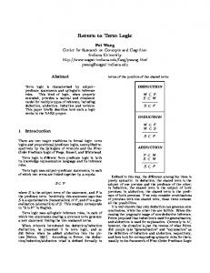
0

Figure 3-2: A non- at poset. Thus, none of these equations are in A. We claim that ()

a = (f (f ))

is not in A0 . The full monotonic lazy model M0 over the base type given in Figure 3-2, where M0[ ]] = 0, M0[ a] = 1, A(M0[ f ] ; 0) = 1, and A(M0[ f ] ; 1) = 2, is a model of A0. It follows that Equation (*) is not in A0, since

M0[ f (f )]] = 2 6= 1 = M0[ a] : The model M0, of course, is not a at lazy model. Nevertheless, any at lazy model satisfying A also satis es Equation (*). This is not hard to prove by a simple case analysis. Let M be a at lazy model satisfying A. If M[ ]] = M[ a] , then M[ f (f )]] = M[ f a] = M[ f ]] = M[ a] where the rst and last equality follow from the fact that a = (f ) holds in the model. If M[ ]] 6= M[ a] , then by monotonicity, M[ a] = M[ f ]] v M[ f (f )]], and so by the atness of the base domain, M[ a] = M[ f (f )]]. In either case M[ a] = M[ f (f )]], so Equation (*) holds for all at lazy models satisfying A. Thus, A0 is incomplete. Even axiomatizing the theory of lazy models (either at or non- at) requires principles beyond inequational logic.

Proposition 3.8 Let A be the set of equations and approximations valid in all lazy models over the simply-typed language with constants ff ! ! ! ; a! ; ! g. Let A0 be the closure, under the usual rules of inequational logic, of the set A [ f v x! g. Then A0 is incomplete (

for all lazy models satisfying A0 .

)

(

)


26

1

Figure 3-3: A poset for giving meaning to terms of type ( ! ).

Proof: For each equation below, there is a lazy model satisfying L that does not satisfy the

given equation:

a = (y a y)

a=

Thus, neither equation is in A. We claim that (y)

(f (f (y a y ))) = (f (x f (y a y ) x))

is not in A0 . To see this, note that a model M0 of A0 exists where the elements of type ( ! ) are assigned meaning in a poset with shape given in Figure 3-3, with M0[ ]] = ?, M0[ a] = 1, M0[ f a] = ?, and M0[ f (y a y)]] = 1. Hence the Equation (y) is not in A0, since

M0[ f (f (y a y))]] = ? =6 1 = M0[ f (x f (y a y) x)]]:

The model M0 is not a lazy model, since the posets on which it is based do not satisfy the conditions for being a lazy type frame. Nevertheless, a simple case analysis shows that any lazy model satisfying A also satis es Equation (y). Let M be any lazy model satisfying A. If M[ f (y a y )]] #, then M[ x f (y a y) x] = M[ f (y a y)]] and hence

M[ f (x f (y a y) x)]] = M[ f (f (y a y))]]:

If M[ f (y a y )]] ", then

M[ f (x f (y a y) x)]] = M[ f (x x)]] = M[ f ]] = M[ f (f (y a y))]]

where the second equality follows from the fact that v a and therefore that M[ f (x x)]] ". Thus, in either case, M satis es Equation (y), which concludes the proof.

3.2. LAZY LOGIC

27

These two examples suggest that reasoning by cases is a fundamental part of reasoning about at lazy models. Sequent logic can be used to capture this reasoning. Sequents have the form (' ` ), where ' and are nite sets of atomic formulas. Appendix A gives a more detailed account of the syntax and semantics of sequents. Lazy logic is a particular sequent logic derived by xing the set of atomic formulas to be convergences, divergences, and approximations of terms, denoted M #, M ", and (M v N ). A lazy sequent is a sequent over these atomic formulas. An atomic formula is closed if its constituent terms are closed; a sequent (' ` ) is closed if all atomic formulas in ' [ are closed. Substitution of terms for free variables also extends to atomic formulas and sets of atomic formulas in the obvious way (by substituting into the constituent terms). The basic axioms and rules of sequent logic appear in Table A.1 of Appendix A. Table 3.1 contains some additional axioms in lazy logic for reasoning about convergences and divergences. For instance, the axiom ( at) captures Proposition 3.3 in the form of a sequent. One of the more important axioms is (div-or-conv), which allows us to reason by cases depending on whether a term diverges or converges. Table 3.2 states the axioms and rules for proving approximations among terms. One may use the lazy axioms and rules as a basis for other lazy logics. Fix some simplytyped language L. A lazy axiom set is a set of lazy sequents whose constituent terms are terms of L. Intuitively, a lazy axiom set is just an additional set of axioms that may be tuned to the particular simply-typed language. A sequent S is lazy provable (often shortened to \provable") from a lazy axiom set if there is a proof tree whose leaves are either sequents in or axioms of lazy logic, and where each step of the proof follows from the inference rules (left-intro), (right-intro), (case), or ( ). Of course, only the terms of the language L may appear in the proof. Figure 3-4 gives an example of a proof in lazy logic using no additional axioms. For practice in using lazy logic, the reader is encouraged to verify the derived rule (conv-cases)

' [ fM #g `

'`

' [ fM "g `

using (div-or-conv) and (case). The usual sequent formulation of consistency extends to the lazy sequent logic: a set of lazy sequents is consistent if the sequent (; ` ;) is not provable from (cf. Appendix A).


28

(div-approx) fM "g ` fM v N g (conv-approx) fM #; (M v N )g ` fN #g (div-or-conv) ; ` fM #; M "g (consis) fM #; M "g ` ; (div-apply)

fM "g ` f(M N ) "g (conv-) ; ` f(x M ) #g ( at) fM #; (M v N )g ` fN v M g

Table 3.1: Rules for reasoning about lazy convergences and divergences.

( -v) ( -w) ( -v) ( -w) (re ) (trans) (cong) ( ) (subst)

; ` f(x M )N v M [x := N ]g ; ` fM [x := N ] v (x M )N g ; ` fM v (x M x)g; x 62 FV (M ) fM #g ` f(x M x) v M g; x 62 FV (M ) ; ` fM v M g fM v M 0; M 0 v M 00g ` fM v M 00g fM v M 0; N v N 0g ` f(M N ) v (M 0 N 0)g ' ` fM v M 0g [ ' ` fx M v x M 0g [ ; x 62 FV (' [ ) '` '[x := M ] ` [x := M ]

Table 3.2: Rules and axioms for approximations in the lazy -calculus.

3.2. LAZY LOGIC

; ` fM "; M #g

29

fM #; (M v N )g ` fN #g fN "; M #; (M v N )g ` fN #g fN #; N "g ` ; fN "; M #; (M v N )g ` ; fN "; M #; (M v N )g ` fM "g fN "; (M v N )g ` fM "g

Figure 3-4: A formal proof of (fN "; (M v N )g ` fM "g) in lazy logic.

3.2.2 Interpretation in at lazy models Sequents and their constituent atomic formulas have a natural interpretation in at lazy models. Suppose M is a at lazy model over a language L and is an M-environment. Let M and N be terms in L. Then M satis es (M v N ) in environment , written M j= (M v N ), i M[ M ] v M[ N ] . A similar interpretation is used for divergences and convergences: M j= (M ") i (M[ M ] ) ", and M j= (M #) i (M[ M ] ) #. Sequents are intepreted as an implication between a conjunction and a disjunction of atomic formulas. Thus, M j= (' ` ) i

M j= for every 2 ' implies that M j= 0 for some 0 2 . We write M j= (' ` ) if M j= (' ` ) for all M-environments (and similarly for atomic formulas). For any lazy axiom set , we write M j= i M j= S for every sequent S 2 . Finally, we write j= S if for all at lazy models M j= , M j= S .

3.2.3 Theorems about lazy sequent logic The two deduction theorems of sequent logic, reviewed in Appendix A, extend to lazy sequent logic.

Theorem 3.9 (Left Deduction) Suppose is a closed atomic formula, and (' ` ) is provable from the set [ f; ` f gg. Then (' [ f g ` ) is provable from . Theorem 3.10 (Right Deduction) Suppose is a closed atomic formula, and (' ` ) is provable from the set [ ff g ` ;g. Then (' ` [ f g) is provable from .

30


Both theorems may be proved by modifying the proofs in Appendix A to account for the ( ) rule, which appears in lazy sequent logic but not in general sequent logics. The following lemma will also be helpful [34]:

Lemma 3.11 Suppose is a lazy axiom set over a simply-typed language L, and let c be a constant not in L. Then the sequent (' ` ) (over the terms in L) is provable from i the sequent ('[x := c] ` [x := c]) is provable from (in the enhanced language). Proof: (Sketch) ()) follows from (subst); (() follows by an easy induction on proof trees.

3.3 Completeness for Flat Lazy Models Lazy logic cannot be used to reach false conclusions in lazy models.

Theorem 3.12 (Soundness of Lazy Logic) Fix a simply-typed language L. Suppose is a lazy axiom set and S is a lazy sequent that is provable from . Then j= S . The proof proceeds by showing that all of the axioms are sound, and that validity is closed under the rules of lazy logic; we give two examples here and leave the proofs of soundness for the other axioms and rules to the reader. For instance, one may verify that the axiom ( -w) is valid in all at lazy models:

Lemma 3.13 j= (fM #g ` fx M x v M g).

Proof: Suppose M is a at lazy model with M j= . Let be any M-environment, and suppose M j= M #. Then M[ M ] #. Note also by the de nition of at lazy model, M[ x M x] #. Now consider any elements d; e with d v e; then

A(M[ x M x] ; d) = M[ M x] [x 7! d] = A(M[ M ] [x 7! d]; M[ x] [x 7! d]) = A(M[ M ] [x 7! d]; d) = A(M[ M ] ; d) v A(M[ M ] ; e)

3.3. COMPLETENESS FOR FLAT LAZY MODELS

31

where the fourth line follows from the fact that x 62 FV (M ), and the last line follows from condition (3) of the de nition of lazy type frame. Thus, it follows from condition (3) of the de nition of lazy type frame that M[ x M x] v M[ M ] , so M j= (x M x v M ) as desired.

Similarly, it is not hard to show that the rule ( ) preserves validity:

Lemma 3.14 Suppose j= (' ` fM v M 0g [ ) and x 62 FV (' [ ). Then j= (' ` fx M v x M 0 g [ ):

Proof: Suppose M is a at lazy model with M j= , and suppose M j= (' ` fM v M 0g[ ). Then for any M-environment , M j= (' ` fM v M 0 g [ ). So suppose is an Menvironment; there are three cases to consider:

1. M 6j= for some 2 ': Then M j= (' ` fx M v x M 0 g [ ) vacuously.

2. M j= for all 2 ' and M j= 0 for some 0 2 : Then it follows easily from the de nition of j= that M j= (' ` fx M v x M 0 g [ ).

3. M j= for all 2 ' and M 6j= 0 for all 0 2 : Since x 62 FV (' [ ), for any element d of M, M j=[x7!d] for all 2 ' and M 6j=[x7!d] 0 for all 0 2 . Since M j=[x7!d] (' ` fM v M 0g[ ) for any d, it must be the case that M j=[x7!d] (M v M 0). We want to prove that M j= (x M v x M 0 ). Note that both M[ x M ] # and M[ x M 0] #, so suppose d v e. Then

A(M[ x M ] ; d) = v v v

M[ M ] [x 7! d] M[ M 0] [x 7! d] A(M[ x M 0] ; d) A(M[ x M 0] ; e)

where the second line follows from the fact above, and the fourth line follows from condition (3) of the de nition of lazy type frame. Thus, M j= (x M v x M 0 ).

Thus, for any , M j= (' ` fx M v x M 0 g [ ). This completes the proof.

32


The soundness theorem and its converse are together called completeness. Completeness tells us that we have not overlooked any necessary logical principles to reason about models. The proof of completeness uses the idea of a \Henkin completion" from rst-order logic [5, 14]. Starting from a lazy axiom set and a sequent S not provable from , the goal is to build a model out of closed terms that satis es but not S . One cannot, however, simply build a model out of the closed, provable approximations of ; it may be the case that an unprovable approximation (M v N ) nevertheless holds when applied to any closed term in the language of . The Henkin completion process overcomes this diculty using witnesses; a witness is an extension of a lazy axiom set by extra constants and axioms so that there are arguments to which we can apply M and N and get dierent results. Thus, when completing the set is nished, we may construct a model from the resultant axiom set that does not satisfy S .

3.3.1 Henkin completion First we need the concept of a witness, which forces an unprovable, closed atomic sequent to be false. (Perhaps a witness is better called a \negative witness," but there will be no corresponding \positive witness.") For some atomic formulas, witnesses are relatively easy to construct. Suppose, for instance, that (; ` fM #g) is not provable from some set of lazy axioms. The witness for this sequent is its negation, the singleton set f; ` fM "gg. Similarly, the witness for (; ` fM "g) is f; ` fM #gg. Constructing witnesses for approximations is more dicult, mainly because lazy logic does not have negated approximations. Suppose the closed sequent (; ` fM v N g) is not provable from . The terms M and N might already be \observably" distinct according to the logic| that is, using the axiom set , M and N could be terms of base type which converge and cannot be proven equal, or M could converge and N diverge. In this case, already witnesses the dierence between M and N . Suppose, on the other hand, M and N have functional type and both converge. Then by lazy extensionality, there should be some term to which we can apply M and N to obtain dierent \observable" behavior. Witnessing the dierence between M and N can be achieved by adding constants to the language together with axioms that force M and N to have dierent behavior. Formally, a witness is an extension to a lazy axiom set.


33

De nition 3.15 Fix a simply-typed language L. Suppose is a consistent lazy axiom set over L and S = (; ` f g) is a closed sequent over L. Let (L0; 0)|a potential witness (there may be more than one)|be one of the following, depending on the form of :

= M #: Let L0 = L and 0 = [ f; ` fM "gg. = M ": Let L0 = L and 0 = [ f; ` fM #gg. = (M v N ): Let c ; : : :; ck (k 0) be fresh constants (with respect to L) and let 1

M 0 = (M c1 : : :ck ) and N 0 = (N c1 : : :ck ). Let L0 be the extension of L to the constants fc1; : : :; ckg (i.e., the least set of terms containing L, fc1; : : :; ckg, and closed under abstraction and application). Then let 0 be either

{ [ f(fM 0 v N 0g ` ;); (; ` fM 0 #g); (; ` fN 0 #g)g, where M 0 and N 0 have type ; or { [ f(; ` fM 0 #g); (; ` fN 0 "g)g. We say that the pair (L0; 0) witnesses S with respect to (L; ) if 0 is consistent. Witnesses may not exist for atomic sequents; that is, there may be no choice of 0 that is consistent. In fact, witnesses do not exist precisely for those closed atomic sequents that are provable from .

Lemma 3.16 Fix a lazy language L. Suppose is a consistent lazy axiom set and S = (; ` f g) is a closed atomic sequent. Then S is provable from i S has no witness with respect to (L; ).

Proof: The direction ()) is straightforward. For ((), suppose S has no witness with respect to (L; ). First suppose that = M ". Since S has no witness with respect to , the set 0 = [ f; ` fM #gg is inconsistent, i.e., (; ` ;) is provable from 0 . By Theorem 3.9, the sequent (fM #g ` ;) is provable from . Hence, by the rule (right-intro) and the axiom (hyp), (fM #g ` fM "g) and (fM "g ` fM "g) are provable from , so by the derived rule (conv-cases) the sequent (; ` fM "g) is provable from . The case when = M # is similar and omitted.

34


Finally, suppose = (M v N ) and M and N have type (1 ! : : : ! n ! ) for n 0. Pick fresh constants ci (with respect to L) of type i . For any 0 k n, let Mk = (M c1 : : :ck ), Nk = (N c1 : : :ck ), and L0 be the extension of L to include the constants fc1; : : :; ck g. We show, for all k, that the sequent (; ` Mk v Nk ) is provable from . The proof will proceed by induction on k, starting with n and working down to 0. This, of course, is enough to prove the lemma, since M0 = M and N0 = N . First consider the basis when k = n. Let 00 = [ f(fMn v Nn g ` ;); (; ` fMn #g); (; ` fNn #g)g 01 = [ f(; ` fMn #g); (; ` fNn "g)g Since S has no witness, both 00 and 01 are inconsistent, that is, (; ` ;) is provable from either 00 or 01. Using this fact, it is not hard to see that each of the following sequents is provable from : 1. (fMn "g ` fMn v Nn g): This sequent is provable from by the axiom (div-approx). 2. (fMn #; Nn #g ` fMn v Nn g): By Theorems 3.9 and 3.10 and the fact that 00 is inconsistent, the sequent (fMn #; Nn #g ` fMn v Nn g) is provable from . 3. (fMn #; Nn "g ` fMn v Nn g): By Theorem 3.9 and the fact that 01 is inconsistent, the sequent (fMn #; Nn "g ` ;) is provable from . Thus, by rule (right-intro), the sequent (fMn #; Nn "g ` fMn v Nn g) is provable from . It follows from the derived rule (conv-cases) that (; ` fMn v Nn g) is provable from . Now consider the induction case when 0 k < n. Let 0 = [ f(; ` fMk #g); (; ` fNk "g)g Since S has no witness, 0 is inconsistent. Therefore, the following sequents are provable from : 1. (fMk "g ` fMk v Nk g): This sequent is provable from by the axiom (div-approx). 2. (fMk #; Nk #g ` fMk v Nk g): By induction, (; ` f(Mk ck+1 ) v (Nk ck+1 )g) is provable from . As ck+1 does not appear in k , by Lemma 3.11 the sequent (; ` f(Mk x) v (Nk x)g)


35

is provable from . By rule ( ), (; ` f(x Mk x) v (x Nk x)g) is provable from , and so using the ( -v), ( -w), and (hyp) axioms, (fMk #; Nk #g ` fMk v Nk g) is provable from .

3. (fMk #; Nk "g ` fMk v Nk g): By Theorem 3.9, the fact that 0 is inconsistent, and rule (right-intro), (fMk #; Nk "g ` fMk v Nk g) is provable from . Using two applications of the derived rule (conv-cases), it follows that (; ` fMk v Nk g) is provable from . This concludes the induction case and hence the proof. Suppose is a consistent lazy axiom set over a simply-typed language L. A completion is built in stages by taking a closed, atomic sequent and either adding it to or adding a witness for it to . More formally, sequents in a completion are built over a simply-typed language L0, which includes the set L (recall from Chapter 2 that L is assumed to be countable), plus a countably in nite set of fresh constants for each type called Henkin constants. Fix some total ordering of the lazy sequents over L0 (this is a countable set of sequents). The stages of the completion are de ned as follows:

Stage 0: Let = and L = L. 0

0

Stage i + 1: Suppose S = (; ` f g) is the ith closed atomic sequent. Let L00 be the set of terms appearing in S , and L000 be the least simply-typed sublanguage of L0 containing Li and L00. If S is provable from i , let i+1 = i [ fS g and Li+1 = L000. Otherwise, pick the pair (Li+1 ; i+1) so that it witnesses S with respect to (L000; i), choosing Henkin constants for the \fresh" constants used in the construction of a witness.

S Finally, let the completion ! = i . (Of course, there may be many completion ! of a lazy axiom set , depending on the ordering of sequents and the witnesses we pick at each stage.) A completion ! is consistent, which follows easily from the following

Lemma 3.17 i is consistent for all i. Proof: An easy induction on i, using the fact that we have a witness at every stage of the construction (which implies that i+1 is consistent).

36


3.3.2 Constructing lazy models from completions For the remainder of the discussion, x a completion ! of a consistent axiom set . Our goal is to construct a at lazy model out of terms that satis es precisely the sequents provable from ! . The posets underlying the model are particularly easy to construct. De ne the relations v on closed terms of type by M v N i (; ` fM v N g) is provable from ! . The relations v induce relations = , where M = N i (M v N ) and (N v M ). Using this de nition of equality,

Lemma 3.18 v is a partial order. Proof: Antisymmetry follows easily from the de nition. Re exivity follows from the (re ) axiom. Similarly, transitivity follows from the (trans) axiom.

De ne T to be the posets composed of = -equivalence classes of closed terms, using [M ] to denote the equivalence class of M . The posets T are partially-ordered, of course, by the natural extension of v to equivalence classes. Divergence is also easy to de ne. If there exists N 2 [M ] such that (; ` fN "g) is in ! , we write [M ] ". Divergence is a well-de ned operation on equivalence classes:

Proposition 3.19 Suppose M 0 2 [M ]. Then the sequent (; ` fM 0 "g) is provable from ! i for all M 00 2 [M ], the sequent (; ` fM 00 "g) is provable from ! . The proof of this proposition uses axiom (div-approx). Finally, de ne application of two equivalence classes [M ] and [P ] by ([M ] [P ]) = [M P ]. This operation is also well-de ned on equivalence classes; the proof uses the (cong) axiom. Now we may put the ingredients together to build a lazy model. Let T = (fT g; f"g; fg). This collection of posets and operations de nes a lazy type frame.

Lemma 3.20 The operators satisfy the lazy extensionality property, i.e., [M ] v [N ] i [M ] # implies [N ] #, and For all [P ], ([M ] [P ]) v ([N ] [P ]).


37

Proof: The ()) direction follows from the derived rule of Figure 3-4 and the axiom (cong). Now suppose [M ] 6v [N ]. Then (; ` fM v N g) is not provable, which by the construction of ! implies that there is a witness for (M v N ). That is, for some sequence of constants ci (possibly null) and terms Mk = (M c1 : : :ck ) and Nk = (N c1 : : :ck ), either 1. (; ` fNk "g) and (; ` fMk #g) are provable, or 2. Mk and Nk are of type , and (; ` fNk #g), (; ` fMk #g), and (fMk v Nk g ` ;) are provable. It follows that (; ` M v N ) cannot be provable: if it were, using (cong), (conv-approx), (consis), and (case), one could prove that ! is inconsistent, which is a contradiction. Therefore, [M ] 6v [N ]. This concludes the (() direction and hence the proof. A T -environment is a type-respecting map from variables to equivalence classes of terms. Note that T -environments are intimately related to substitutions, which are maps from variables to terms. Substitutions can be naturally extended to terms, i.e., if ~x contains the free variables of M and is a substitution, then (M ) = M [~x := (~x)], where M [~x := (~x)] denotes the simultaneous substitution of (xi ) for xi .

De nition 3.21 Let be a T -environment. A substitution represents if for all variables x, (x) 2 (x). Lemma 3.22 T is a at lazy model under the meaning function T [ M ] = [(M )], where is any substitution representing .

Proof: First we verify that T is a at lazy type frame. Part (1) of the de nition of at lazy

model follows from axiom (div-approx), Part (2) follows from axiom (div-apply), and Part (3) follows from Lemma 3.20. Flatness follows follows from the axiom ( at). We therefore only need show that T [ ] satis es the equations given in the de nition of a at lazy environment model. But

T [ x] = [(x)] = (x)


38

T [ M N ] = [(M N )] = [(M )] [(N )] = (T [ M ] ) (T [ M ] ) For -abstractions, (T [ x M ] ) [N ] = [(x M )] [N ]

= [((x M ) N )]

= [(M [x := N ])] = T [ M ] [x 7! [N ]] where the second equality follows from the de nition of and the fact that N is closed, and third equality follows from the axioms ( -v)and ( -w). This completes the proof. Using a completion to construct the model is important precisely because all closed atomic formulas witnessed by ! are denied in T .

Lemma 3.23 Suppose S = (; ` f g) is not provable from ! . Then T 6j= . Proof: If = M ", then by the construction of ! , (; ` fM #g) is provable from ! . Thus, T 6j= S . The argument is similar if = M #. Finally, the case when = (M v N ) follows along the same lines as the proof of Lemma 3.20.

We may now prove the main completeness theorem.

Theorem 3.24 (Completeness for Flat Lazy Models) Let L be a simply-typed language,

and suppose is a lazy axiom set and S is a sequent over L. Then S is provable from i j= S .

Proof: The direction ()) is soundness. For ((), suppose S = (' ` ) is not provable from , where FV (S ) = fx ; : : :; xng. We begin by making S a closed sequent. Choose fresh constants 1

c1; : : :; cn not appearing in L. Let '0 = '[~x := ~c ] and 0 = [~x := ~c ]. By Lemma 3.11, S 0 = ('0 ` 0) is not provable from . Let 0 = [ f(; ` ) : 2 '0g [ f( 0 ` ;) : 0 2 0g:

3.4. THEORY OF LAZY PCF

39

We claim that 0 is consistent: if not, the sequent (; ` ;) is provable from 0 , and so by Theorems 3.9 and 3.10, the sequent S 0 is provable from , which is a contradiction. Let ! be a completion of 0, and let T be the associated term model. By Lemma 3.22 T j= ! and so T j= . Note that for all 0 2 0, (; ` f 0g) is not provable from ! |if it were, then since (f 0g ` ;) 2 ! , the sequent (; ` ;) would be provable from ! by rule (case), which contradicts the fact that ! is consistent. By Lemma 3.23, T 6j= 0 for all 0 2 0. Thus, T 6j= S 0, since T j= for all 2 '0 but T 6j= 0 for all 0 2 0. This term model T also denies S : one can pick an environment (namely, any environment which assigns a variable xi to the T -meaning of ci ) such that T 6j= S . Thus, T 6j= S , which completes the proof.

3.4 Theory of Lazy PCF The denotational and axiomatic theory developed above is a general theory of lazy languages. We now apply this general theory to a speci c language, lazy PCF, by building a fully abstract denotational model. This model will be a lazy model, and hence the logic will be sound for proving facts about lazy observational congruences and approximations.

3.4.1 Review of the essentials of domain theory We rst review the concepts of complete partial orders, continuous functions, and isolated elements from domain theory. Suppose D is a poset. If d and e are elements of D, the least upper bound of d and e, provided it exists, is written d t e. If d and e have an upper bound, they are said to be consistent. A subset X D is directed if for any pair of elements x; y 2 X , x and y are consistent. We say that D is a complete partial order (cpo) if for any F directed X D, ( X ) exists and is in D. A monotone function f : D ! E , where D and E F F are cpo's, is continuous if for any directed set X D, f ( x2X x) = x2X f (x). The poset [D !c E ] is the set of continuous functions ordered pointwise. If D and E are cpo's, [D !c E ] is also a cpo. Likewise, if D and E are pointed, [D !c E ] is pointed. Isolated elements are the building blocks of the cpo's. Suppose D is a cpo; then an element d 2 D is isolated (elsewhere called nite [41] or compact [22]) if for any directed set X , d vD (F X ) implies d v x for some x 2 X . A poset D is algebraic if for any d 2 D,


40

d = Ffe : e v d and e is isolatedg. Isolated elements in algebraic posets thus ll the same role

as rational numbers do in the case of the real numbers: that is, as any real can be de ned as a sequence of better and better rational approximations, an element of an algebraic cpo can be expressed as a sequence of better and better isolated approximations. All of the posets of this chapter will be Scott domains, viz., consistently-complete3 algebraic cpo's whose set of isolated elements is countable [22, 53]. For example, all elements of N? , the at cpo of natural numbers, are isolated. The isolated elements of [D !c E ], where D and E are Scott domains, are least upper bounds of nite sets of threshold functions. These threshold functions are often written in the form (d ) e), where d and e are isolated and 8 > < e if d v d0 0 (d ) e)(d ) = > : ? otherwise.

3.4.2 Denotational semantics for lazy PCF Finding a suitable intepretation for recursion is the main diculty in building a denotational model of lazy PCF. By restricting the class of functions to the continuous functions, it possible to interpret recursion via least xpoints [51, 67]. The use of continuous functions also has a purely operational justi cation: a term cannot return a dierent answer based on an \in nite" amount of information than it returns based on all \ nite" approximations. For instance, consider the terms

F0 = x cond x 1

F1 = x cond x 1 (cond (pred x) 1 ) F2 = x cond x 1 (cond (pred x) 1 (cond (pred (pred x)) 2 ))

.. .

Intuitively, each Fi : ( ! ) is a nite version of the factorial function; it can compute the factorial of all numbers i, but will diverge on numbers > i. Let F be any term representing the factorial function and let M be a term of type (( ! ) ! ), and suppose (M F ) halts. 3 A poset is consistently-complete if for any pair of elements x and y with an upper bound, x and y have a least upper bound. This notion will be unimportant here.


41

L[ x ] = (x) L[ n] = n

L[ x M ] = lift(g); where g(d) = L[ M ] [x 7! d] L[ M N ] = (G L[ M ] ) l (L[ N ] ) L[ x M ] = f n (?); where f (d) = L[ M ] [x 7! d]

L[ conv M N ] = L[ succ M ] =

n0

(

(

8 > < L[ pred M ] = > : 8 > < L[ cond M N P ] = > : 8 > > < L[ pcond M N P ] = > > :

?

if [ M ] = ? [ N ] otherwise

? if L[ M ] = ? L[ M ] + 1 otherwise ?

if L[ M ] = ? if L[ M ] = 0 L[ M ] ? 1 otherwise

0

L[ N ] if L[ M ] = 0 L[ P ] if L[ M ] > 0 ? otherwise L[ N ] L[ P ] L[ P ] ?

if L[ M ] = 0 if L[ M ] > 0 if L[ N ] = L[ P ] otherwise

Table 3.3: Equations for interpreting lazy PCF terms. Here, ? denotes the least element in the appropriate domain. Abusing notation, we write n for both the numeral denoting n and the natural number n itself. During this process, M can only test F at a nite number of places. Hence, (M Fi ) must also converge for all i n, where n is some xed value. The lazy type frame for lazy PCF is built out of lifted continuous functions. Let L = N? and L! = [L !c L ]? , " = f?g, and A(d; d0) = d l d0 = drop(d)(d0). Table 3.3 gives semantic equations for interpreting LPCF-terms. The continuous lazy model is both adequate and fully abstract.

Theorem 3.25 (Bloom and Riecke [9]) The model L satis es the following properties: 1. Adequacy: If M is closed, then M +l i L[ M ] 6= ?, and M +l k i L[ M ] = k;


42

2. Inequational Full Abstraction: M vlazy N i for all environments , L[ M ] v L[ N ] .

We will make extensive use of this theorem and the model L in Chapter 5. We pursue the proof of adequacy in detail and give a sketch of the proof of full abstraction. One direction of adequacy, the ()) direction, follows easily from the following two lemmas:

Lemma 3.26 For any LPCF terms P and Q, L[ P ] [x 7! L[ Q] ] = L[ P [x := Q]]]. Proof: (Sketch) By induction on the structure of P (cf. [4]). Lemma 3.27 If M is closed and M +l V , then L[ M ] = L[ V ] . Proof: By induction on the proof of M +l V . In the basis, M = V +l V ; then it follows trivially that L[ M ] = L[ V ] . In the induction step, there are eleven cases depending on the last rule used. We consider a few examples here and leave the others to the reader to verify. 1. M = (succ P ), where P +l k. By induction, L[ P ] = L[ k] , so

L[ M ] = (L[ P ] ) + 1 = (k + 1) = L[ V ] as desired. 2. M = (P Q), where P +l (x P 0 ) and P 0 [x := Q] + V . Then

L[ M ] = (L[ P ] l L[ Q] ) = (L[ x P 0 ] l L[ Q] ) = L[ P 0 ] [x 7! L[ Q] ] = L[ P 0 [x := Q]]] = L[ V ]

where the second and fth lines follow from the induction hypothesis, and the fourth line follows from Lemma 3.26. This completes the induction case and hence the proof. The (() direction of adequacy requires a much dierent technique. We use an inclusive predicate approach here, following the proofs of adequacy given in [10, 21]. First, we de ne a relation between elements of the model L and closed terms M .


43

De nition 3.28 For d 2 L and M a closed LPCF-term of type , we say that d either d = ?, or M +l V and d V , where

.

M if

.

1. k k; and .

2. f

.

! ) (x P ) i

(

for every e Q, (f l e) ((x P ) Q). .

.

The goal is to show that for any closed M , ()

L[ M ]

.

M:

From this it will be easy to conclude the (() direction of adequacy. To handle recursion properly, we rst need a condition on the relations : .

Lemma 3.29 If d v d v d v : : : and di 0

1

2

.

M for all i 2 N, then (F di )

.

M.

Proof: By induction on types. First consider the basis, when = . If (F di) = ?, then F F 6 ?, then some d 6= ? and hence M + V follows from the fact that ( di ) M . If ( di ) = j l F dj M . Also, since L is a at poset, ( di ) = dj . Thus, since dj M , it follows that .

.

F ( d) i

.

.

M as desired.

F Now consider the induction step when = ( ! ). Again, if ( di ) = ?, then F F ( di ) M . If, on the other hand, ( di) 6= ?, then some dj 6= ? and hence M +l V . Now suppose e Q. Then (di l e) (V Q), and hence by induction .

.

.

G G ( (di l e)) = (( di) l e) (V Q): .

F F F If (( di ) l e) = ?, then (( di ) l e) (M Q). If (( di) l e) 6= ?, then for some dj , it F must be that (dj e) 6= ?. Thus, (V Q) + V 0 and (( di) l e) V 0 . But then (M Q) +l V 0, F F so (( di ) l e) (M Q) as required. Thus, ( di ) M . .

.

.

.

The main lemma of the adequacy proof is a generalization of () to open terms.

Lemma 3.30 Suppose M is an LPCF-term of type whose free variables are contained in ~x and di i Ni . Then L[ M ] [~x 7! d~] M [~x := N~ ]. .

.


44

Proof: By induction on the structure of M . In the basis, M is either a numeral k or a variable xi . If M = k, then

L[ M ] [~x 7! d~] = k If M = xi , then

L[ M ] [~x 7! d~] = di

.

.

k = M [~x := N ~ ]:

i

Ni = M [~x := N~ ]

by hypothesis. There are eight cases in the induction step. We consider the three dicult cases and leave the others to the reader: 1. M = (P Q). Let f = L[ P ] [~x 7! d~] and e = L[ Q] [~x 7! d~], and P 0 = P [~x := N~ ] and Q0 = Q[~x := N~ ]. Our goal is to show that (f l e) (P 0 Q0). By the induction hypothesis, f ( !) P 0 and e Q0. If f = ?, then (f l e) = ? and hence (f l e) (P 0 Q0). If f 6= ?, it must be the case that P 0 +l (x P 00 ) and f ( !) (x P 00 ). By the de nition of , (f l e) ((x P 00 ) Q0): .

.

.

.

.

.

.

If (f l e) = ?, then (f l e) (P 0 Q0 ) automatically. If (f l e) 6= ?, then it follows that ((x P 00 ) Q0 ) +l V and (f l e) V . But note that (P 0 Q0 ) +l V , and hence (f l e) (P 0 Q0) as desired. .

.

.

2. M = (y P ), where = ( ! ) and y 62 ~x. Let f = L[ M ] [~x 7! d~] and M 0 be the term M [~x := N~ ]. Clearly, M 0 +l M 0 . Suppose e Q; we must show (f l e) (M 0 Q). If (f l e) = ?, then (f l e) (M 0 Q). Otherwise, if (f l e) 6= ?, then note that

.

.

.

(f l e) = .

L[ P ] [~x 7! d~; y 7! e] P [~x := N~ ][y := Q]

where the last line follows from the induction hypothesis. Since (f l e) 6= ?, it must be the case that P [~x := N~ ][y := Q] +l V and (f l e) V . But then (M 0 Q) +l V , so (f l e) (M 0 Q) as desired. .

.

3. M = (y P ), where y 62 ~x. Let P 0 = P [~x := N~ ] and M 0 = y P 0 , and de ne e0 = ? and ei+1 = L[ P ] [~x 7! d~; y 7! ei ]. We shall prove that for all i, ei M 0 . In the basis,

.

3.4. THEORY OF LAZY PCF e0

.

45

M 0 since e0 = ?. Now suppose ei

lemma,

.

M 0 . By the induction hypothesis of the

ei+1 = L[ P ] [~x 7! d~; y 7! ei]

.

P 0 [y := M 0]

If ei+1 = ?, then ei+1 M 0. If ei+1 6= ?, then P 0 [y := M 0 ] +l V with ei+1 V . But then M 0 +l V , and hence ei+1 M 0 . F Let e = ( ei ) = L[ M ] [~x 7! d~]; then by Lemma 3.29, e M 0 as desired. .

.

.

.

This completes the induction step and hence the proof.

Proof of Theorem 3.25: The ()) direction of adequacy follows directly from Lemma 3.27. For the (() directions, note rst that L[ M ] M by Lemma 3.30. Thus, if L[ M ] = 6 ?, M +l as desired. Similarly, if L[ M ] = k, then M + k. The (() direction of full abstraction follows from adequacy (cf. [41]). For the more complicated direction ()), suppose L[ M ] 6v L[ N ] . If ~x contains all the free variables of M and N , then L[ ~x M ] 6v L[ ~x N ] . By the properties of Scott domains, there must be a sequence of isolated elements di such that f = (L[ ~x M ] l d l : : : l dn ) = 6 ? and g = (L[ ~x N ] l d l : : : l dn ) = ?, or f and g are dierent numbers. It is possible to .

1

1

show that all isolated elements are de nable (using a proof similar to the proof given in [41] which is omitted) using LPCF-terms in the syntax

M ::= x j n j j (x M ) j (M M ) j (succ M ) j (pred M ) j (cond M M M ) j (pcond M M M ) j (conv M M )

where is an abbreviation for (x x). This set of terms is called ILPCF|for Isolated LPCF. Therefore, by Part (1), there is a sequence of arguments Di such that ((~x M ) D~ ) and ((~x N ) D~ ) yield dierent lazy observations. Thus, M 6vlazy N .

3.4.3 Relationship to lazy theory It is not dicult to prove that L is a at lazy model; this follows easily from the following

Lemma 3.31 For any term M of type , 1. L[ M ] 2 L ; and


46

F

F

2. For any directed set fdi : i 2 I g, L[ M ] [x 7! ( di )] = (L[ M ] [x 7! di].

Proof: (Sketch) By induction on the structure of M . Part (2) is an induction hypothesis

necessary to make Part (1) go through in the -abstraction case.

Therefore, lazy logic is sound for proving approximations in L|and hence by Theorem 3.25, the logic is sound for proving observational congruences in the lazy PCF. In the case of call-by-name PCF, however, there is a more intimate connection between the fully abstract model N (de ned in Appendix B) and its logic, -equality.

Theorem 3.32 (Plotkin [43], Statman [63]) Suppose M and N are pure terms (that is, terms containing no recursion, conditionals, numerals, or arithmetic). Then N j= (M v N ) i M and N are provably equivalent using -reasoning.

Thus, by the full abstraction theorem for N , -equality is complete for proving observational approximations between pure terms in call-by-name PCF. This is an important theorem, for it further demonstrates that -equality is a good basis for reasoning about call-by-name PCF. A similar theorem should hold for lazy logic.

Conjecture 3.33 For any pure LPCF-terms M and N , L j= (M v N ) i (; ` M v N ) is provable in lazy logic.

We retract the announcement of this result made in [12].

3.4.4 Recursion-free approximations are co-r.e. Given the completeness conjecture, it would follow that the pure approximations valid in the continuous model are r.e., and hence by the following theorem the approximations valid in the continuous model would be decidable:

Theorem 3.34 The following question is r.e.: Given any ILPCF-terms M and N , is it the case that L[ M ] 6v L[ N ] for some environment ? The proof of Theorem 3.34 relies upon an evaluator for ILPCF-terms, whose de nition appears in Table 3.4. The canonical terms (denoted c) of this interpreter are values and , so does not diverge in the modi ed interpreter. The new evaluator incorporates a few changes when

3.4. THEORY OF LAZY PCF c+c M +0 (pred M ) + 0

M +V0 N +V (conv M N ) + V M + (n + 1) P + V (cond M N P ) + V M +0 N +k (pcond M N P ) + k M + N +c P +c (pcond M N P ) + c M +

(M N ) +

47

M +n (succ M ) + (n + 1) M + (n + 1) (pred M ) + n M +

(conv M N ) +

M +0 N +V (cond M N P ) + V M + (n + 1) P + V (pcond M N P ) + V M + N + c P + c0 c 6= c0 (pcond M N P ) +

M + x M 0 M 0[x := N ] + V (M N ) + V

M +

(succ M ) +

M +

(pred M ) +

M +

(cond M N P ) +

Table 3.4: Interpreter for ILPCF. compared with the original lazy PCF interpreter of Chapter 2; the term (succ ), for instance, reduces to since its meaning is ?. Our goal is to show that all terms in this language halt under the modi ed interpreter, and then use the evaluator in an algorithm for testing whether two recursion-free terms do not approximate each other. We use Tait's computability method [41, 68] to prove that all terms halt under the modi ed interpreter. First,

De nition 3.35 A closed term M is stoppable if either 1. M is of type , and M + c for some canonical c; or 2. M is of type ( ! ), and M + c for some canonical c, and for any stoppable N , (M N ) is stoppable. An open term M is stoppable if any instantiation M 0 of M by closed, stoppable terms is stoppable.


48

Lemma 3.36 A closed term M is stoppable i for all closed stoppable terms Ni with k 0, (M N : : : Nk ) + c for some canonical c. 1

Proof: An easy induction on types. Thus, the intuitive idea behind a stoppable term is captured by its name|a stoppable term always halts whenever applied to stoppable terms.

Lemma 3.37 All terms are stoppable. Proof: Pick any term M ; we proceed by induction on the structure of M . In the basis, M is ei-

ther a numeral k, a constant , or a variable x. Obviously k is stoppable. Likewise, a variable x is stoppable, since any instantiation of x by a closed stoppable term is stoppable. The only case left is M = . Note, however, that for any closed stoppable terms Ni, ( N1 : : :Nk ) + . Thus, by Lemma 3.36, is stoppable. There are a number of cases in the induction step. We consider three illustrative cases: 1. M = (succ N ): Consider any instantiation M 0 = (succ N 0 ) of M by closed stoppable terms. Since N is stoppable by induction, N 0 is stoppable. Thus, either N 0 + k for some numeral k or N 0 + , and so either M 0 + (k + 1) or M 0 + . This shows that M 0 is stoppable, and hence M is stoppable. 2. M = (P Q): Let M 0 = (P 0 Q0 ) be any instantiation of M by closed stoppable terms. Since both P and Q are stoppable by induction, by de nition P 0 and Q0 are stoppable. Thus, (P 0 Q0 ) is stoppable since P 0 is stoppable, closed, and of functional type, and hence M is stoppable. 3. M = (x P ): Let M 0 = (x P 0 ) be any instantiation of M by closed stoppable terms. By induction, P is stoppable, so P 0 is stoppable. First note that M 0 + M 0 . Now consider any closed stoppable terms Ni. Then P 0 [x := N1 ] is an instantiation of P by closed stoppable terms, and hence ((P 0 [x := N1 ]) N2 : : :Nk ) + by Lemma 3.36. Thus, (M 0 N1 : : : Nk ) +, and hence by Lemma 3.36, M 0 is stoppable as desired.


3.5. CONCLUSION

49

Proof of Theorem 3.34: There are two important facts that hold for the model L: 1. The isolated elements of each Scott domain L can be recursively-enumerated [22, 41]; and

2. If x1 ; : : :; xn is a list of all free variables in M and N , and L[ ~x M ] 6v L[ ~x N ] , then there is a sequence of isolated elements di such that either f = (L[ ~x M ] l d1 l : : : l dk ) is not ? and g = (L[ ~x N ] l d1 l : : : l dk ) is ?, or f and g are distinct natural numbers.

The algorithm works as follows: choose a sequence of isolated elements di, encode them as Di in the restricted syntax of ILPCF (which is possible by the proof of Theorem 3.25), and evaluate the terms M 0 = ((~x M ) D1 : : :Dk ) and N 0 = ((~x N ) D1 : : :Dk ). By Lemma 3.37, these evaluations must halt at either a value V or . If N 0 + and M 0 does not, or they evaluate to dierent numerals, halt and say \yes;" the terms M 0 and N 0|and hence the terms M and N |are semantically dierent, since the model L is sound for the evaluator. If not, continue with another sequence of isolated elements. This procedure answers \yes" i L[ M ] 6v L[ N ] , for some environment , by the two properties above.

3.5 Conclusion We have shown that some of the important characteristics of the call-by-name theory carry over to the lazy setting, i.e., there is a logic (like the logic of ) that is complete for proving facts in all models of lazy languages. There are some dierences, however: we had to give up equational reasoning in favor of sequents and needed to reason explicitly about approximations, divergences, and convergences. Another dierence arises from the distinction between sequential and parallel languages. Theorem 3.32 shows that vname coincides with -equality on pure terms. Call-by-name observational congruence in the sequential version of PCF (the language without parallel conditional) on pure terms also coincides with -equality. The proof, due to Albert Meyer, follows from a simple term model construction for sequential call-by-name PCF and Statman's one-section theorem [63], which states a general condition on when -equality is complete for reasoning about a model. Thus, for pure terms, sequential and parallel call-by-name observational congruence theories are identical.


50

In contrast to the classical case, however, there is a dierence between sequential PCF and LPCF contexts. The following counterexample is due to Kurt Sieber [56]:

Example 3.38 (Sieber) Consider the pure terms P1 = f g x f (f (g x) (g x)) (f (g x) (g x)) P2 = f g x f (f (g x) (g (y x y))) (f (g (y x y)) (g x))

where f has type ( ! ! ), g has type (( ! ) ! ), and x has type ( ! ). Then P1 and P2 are congruent in sequential lazy PCF but P1 6lazy P2 .

Proof: For any f programmable in (sequential) PCF, f is either strict in one of its arguments

or is a constant function. A case analysis shows that P1 and P2 are sequential congruent. However, if Q1 is the term that tests either of its arguments for 0 and returns 0 if either is 0, Q2 is the convergence testing function that returns 0 if its argument converges, and Q3 diverges, then (P1 Q1 Q2 Q3 ) diverges while (P2 Q1 Q2 Q3) returns 0. Note that Q1 , Q2, and Q3 are programmable in LPCF; hence, P1 6lazy P2 . Given the problems associated with nding suitable sequential models (cf. [6, 37]) for these languages, we expect the problem of axiomatizing sequential lazy observational congruence| even on pure terms|to be dicult. We have shown that the pure approximations in L are co-r.e, and conjectured that the pure approximations are r.e. as well. This would imply that the pure approximations holding in L|and hence the pure observational approximations for lazy PCF|are decidable. But this decision procedure sheds no light into the complexity of deciding validity of pure equations. Indeed, the decision procedure for -equality between pure terms has an iterated-exponential upper and lower bound [61]. An iterated-exponential lower bound for lazy logic can be deduced from Statman's results. The upper bound remains unknown. One might also want extended logics for proving lazy congruences in richer languages. Certain extensions to the type structure, e.g., non-recursive type-constructors like pairing, sum, and lifting (which plays a distinguished role in the lazy theory of [11]), should not be problematic, but we have not yet tried to develop these extensions.

Chapter 4

Models and Logics of Call-by-value Languages To supplement operational reasoning in call-by-value languages, it is useful to have a denotational and axiomatic semantics. This chapter develops the denotational and axiomatic theory of call-by-value languages, which diers only in a few respects with the denotational and axiomatic theory of lazy languages developed in Chapter 3. We rst de ne the notions of a at call-by-value model and call-by-value logic, and prove a completeness theorem that shows the correspondence of these denotational and logical theories. We then de ne an adequate and inequationally fully abstract model for call-by-value PCF, and brie y discuss its relationship to the logic. We also prove, using the model, that observational approximation between terms in a subset of call-by-value PCF is co-r.e. Although most of the proofs of this chapter are similar to the previous chapter, we develop most of them in full.

4.1 Models of Call-by-value Languages Call-by-value languages share certain operational properties. Many of these properties, like lazy extensionality, monotonicity, and atness carry over from the lazy case. Consider, for instance, the language call-by-value PCF:

Proposition 4.1 Let M and N be closed PCF-terms of type ( ! ). Then M vval N i M +v implies N +v , and for any closed P , (M P ) vval (N P ). 51

52

CHAPTER 4. MODELS AND LOGICS OF CALL-BY-VALUE LANGUAGES

This could be called call-by-value extensionality, but it is the same as lazy extensionality. The proof of the proposition can be carried out purely syntactically or by appealing to the fully abstract denotational model V de ned below. Similarly, one can prove that, with respect to the ordering vval , functional terms are monotone and the base type is at. One important property that distinguishes call-by-value from lazy languages is the reduction of applications. In a call-by-value language, if an operand diverges, the entire application must diverge. The denotational concept of strictness is strongly related to this behavior of call-byvalue languages. Let D and E be pointed posets (recall that a pointed poset is one with a least element) with least elements ?D and ?E . A function f from D to E is strict if f (?D ) = ?E . Functions in call-by-value languages are strict: since the least element ? is the meaning of any divergent term, the meaning of a call-by-value function should send ? to ?. The poset of strict functions from D to E ordered pointwise is denoted [D !s E ]. Since we will also at times require monotonicity, we will denote the set of strict monotone functions from D to E as [D !s;m E ]; likewise, the poset of strict, continuous functions ordered pointwise is denoted [D !s;c E ]. There is also a canonical way to turn an arbitrary function f between two pointed posets into a strict function: 8 > < ? if d = ? strict(f )(d) = > : f (d) otherwise.

4.1.1 Call-by-value environment models The principles of lazy extensionality, monotonicity, atness, and strictness all play a crucial role in the de nition of a call-by-value denotational model. There are two components to a call-by-value model: a call-by-value type frame, which de nes spaces of possible meanings, a divergence predicate, and an abstract application operator; and a meaning function that assigns meaning to terms. First,

De nition 4.2 A call-by-value type frame is a tuple (fD g; f"g; fA; g), where each D is a poset, " D , and A; : D ! D ! D . We write d " whenever d 2", and d # whenever d 62". The components of a call-by-value type frame must also obey the following properties: 1. If d ", then d v e for all e 2 D ;

4.1. MODELS OF CALL-BY-VALUE LANGUAGES

53

2. If either d " or e ", then A(d; e) "; and 3. f vD ! g i f # implies g #, and for all d vD e, A(f; d) vD A(g; e). A at call-by-value type frame is a call-by-value type frame in which D is either discretelyordered or D = E? for some discretely-ordered E . Call-by-value type frames dier from lazy type frames only in clause (2) of the de nition: if either the rst or the second argument to A diverges, then the result diverges. This re ects the call-by-value parameter-passing mechanism, and is a more general characterization of strictness (it is more general because the set " may be empty). Second, there is a meaning function that assigns meaning to terms based on their structure. As in Chapter 3, free variables are given meaning via environments:

De nition 4.3 Let (fD g; f"g; fA; g) be a call-by-value type frame. A D-environment is a map from variables to elements of D where (x ) 2 D . De nition 4.4 Let L be any simply-typed language. A call-by-value environment model for L is a call-by-value type frame D with a meaning function [ ] , such that the meaning function satis es the equations

[ x ] = (x ) [ (M N )]] = A([[M ] ; [ N ] ) [ x M ] = f; where f # and for any d such that d #, A(f; d) = [ M ] [x 7! d]

and where [ M ] 2 D for any L-term M of type . A at call-by-value model is a call-byvalue model based on a at call-by-value type frame. Given any call-by-value environment model, the meaning of a closed term is independent of the choice of environment, i.e., if M is closed, then [ M ] = [ M ] 0 for any environments and 0. Therefore, for brevity, the environment will often be dropped when describing the meaning of a closed term. The connection between lazy and call-by-value environment models means that the de nition of \call-by-value model" is quite close to Abramsky's [2, 3] and Ong's [39] de nitions of lazy models. It also is related to Moggi's de nition of call-by-value models [34], but there

54


are two signi cant dierences. First, variables may never be bound to divergent elements in Moggi's de nition of an environment; according to the de nition here, they may be. This change simpli es the logic, but it also is necessary in the case of interpreting call-by-value PCF. For instance, under Moggi's de nition of model, the equation x = (y x y ) always holds, but in call-by-value PCF, x 6val (y x y ): the context (x []) causes x to diverge and (y x y ) to converge. Second, the de nition here incorporates atness, which Moggi's de nition omits. Indeed, the class of models with at base types satisfy more approximations than those without; a precise example will be given later when we consider the logic of call-by-value PCF.1

4.1.2 Examples of call-by-value models Many call-by-value type frames t the conditions for being a model. For example, the full lifted, strict monotonic type frame over N? , de ned

F = N? F ! = [F !s;m F ]? " = f?g A; (f; d) = drop(f )(d) is one example of a call-by-value model over the simply-typed language with no extra constants or constructs. That is, the equations in the de nition of model uniquely determine a meaning function F [ ] such that F [ M ] 2 F for any M of type . The classical set-theoretic model over a set B , de ned by the frame

S = S S ! = [S ! S ] " = ; A; (f; d) = f (d) is also a call-by-value model for the language with no constants or other constructs. (Each poset in this model is discretely-ordered.) 1 The reader familiar with Moggi's models may also remember that they are based on partial rather than total functions, but this dierence is unimportant.

4.1. MODELS OF CALL-BY-VALUE LANGUAGES

55

fM "g ` fM v N g (conv-approx) fM #; (M v N )g ` fN #g ; ` fM #; M "g (consis) fM #; M "g ` ; (div-apply) fM "g ` f(M N ) "g (conv-) ; ` f(x M ) #g (div-operand) fN "g ` f(M N ) "g ( at) fM #; (M v N )g ` fN v M g

(div-approx) (div-or-conv)

Table 4.1: Rules for reasoning about convergences and divergences of -terms in call-by-value, where c ranges over constants.

( v -v) ( v -w) ( -v) ( -w) (re ) (trans) (cong) ( )

fN #g ` f(x M )N v M [x := N ]g fN #g ` fM [x := N ] v (x M )N g ; ` fM v (x M x)g; x 62 FV (M ) fM #g ` f(x M x) v M g; x 62 FV (M ) ; ` fM v M g f(M v M 0); (M 0 v M 00)g ` fM v M 00g f(M v M 0); (N v N 0)g ` f(M N ) v (M 0 N 0)g ' ` fM v M 0g [ (' ` fx M v x M 0g [ ; x 62 FV (' [ ) '` '[x := M ] ` [x := M ]

(subst)

Table 4.2: Rules and axioms for call-by-value approximations.

56


4.2 Call-by-value Logic Call-by-value logic has the same avor as lazy logic; we again use sequents of approximations (M v N ), convergences M #, and divergences M " as a basis. Table 4.1 gives basic axioms about divergence and convergence of terms, and Table 4.2 details more axioms dealing speci cally with approximations. For example, (div-or-conv) states that every term either converges or diverges. The axiom (consis) states that a term cannot both converge and diverge. Most of these axioms appear elsewhere; see [34], for example.2 The key axiom missing from most axioms systems is the axiom ( at), which states that the base type is at. The essential dierences between call-by-value logic and lazy logic lie in the (div-operand), ( v -v), and ( v -w) axioms. Lazy logic does not include the (div-operand) axiom, since applications in lazy languages may converge even though their operands diverge. This fact is re ected in the ( v -v) and ( v -w) axioms as well: in lazy languages, one need not show that the argument converges before substituting it for a formal parameter.

4.2.1 Interpretation in at call-by-value models The interpretation of call-by-value sequents in call-by-value models is much the same as for lazy sequents in lazy models. Suppose M is a at call-by-value model for the language L, and is an M-environment. Then M j= (M v N ) i M[ M ] v M[ N ] . Similarly, M j= (M ") i (M[ M ] ) ", and M j= (M #) i (M[ M ] ) #. Sequents are interpreted as implications from conjunctions to disjunctions. Thus, M j= (' ` ) i

M j= for every 2 ' implies M j= 0 for some 0 2 . We write M j= (' ` ) if for all M-environments , M j= (' ` ). Finally, for a call-by-value axiom set (i.e., a set of call-by-value sequents), we write M j= i M j= S for every sequent S 2 , and j= S i for all M j= , M j= S . 2 Moggi's logics in [34] are more complicated than ours; in particular, he builds in extensionality as an axiom using quanti cation.

4.3. COMPLETENESS FOR FLAT CALL-BY-VALUE MODELS

57

4.2.2 Theorems about call-by-value sequent logic The usual deduction theorems of sequent logic hold in call-by-value logic.

Theorem 4.5 (Left Deduction) Suppose is a closed atomic formula, and (' ` ) is provable from the set [ f; ` f gg. Then (' [ f g ` ) is provable from . Theorem 4.6 (Right Deduction) Suppose is a closed atomic formula, and (' ` ) is provable from the set [ ff g ` ;g. Then (' ` [ f g) is provable from . The proofs of these two theorems are identical to the proofs of the corresponding deduction theorems from Chapter 3. One may also change free variables into constants using the following lemma:

Lemma 4.7 Suppose is a call-by-value theory over a simply-typed language L, and let c be a constant not in L. Then the sequent (' ` ) (over the terms in L) is provable from i the sequent ('[x := c] ` [x := c]) is provable from (in the enhanced language).

4.3 Completeness for Flat Call-by-value Models Call-by-value logic cannot be used to derive false conclusions in at call-by-value models.

Theorem 4.8 (Soundness of Call-by-value Logic) Fix a simply-typed language L. Suppose is a call-by-value sequent theory, and S is provable from . Then j= S . The proof is not dicult and hence is omitted; one proceeds by induction on the length of the proof of S , showing that each axiom of call-by-value logic holds in every at call-by-value model, and that the rules preserve validity. Soundness and its converse, together called completeness, demonstrate the intimate connection between the class of call-by-value models and the call-by-value logic. The proof of completeness follows the same ideas as the proof of Theorem 3.24 given in Chapter 3: given a call-by-value axiom set and a sequent S not provable from , we construct a completion set ! which provides witnesses for all closed, unprovable atomic sequents, and also does not prove S . From the completion set we can construct a term model that satis es but denies S .

58


4.3.1 Henkin completion Witnesses to atomic sequents have the same formulation as before.

De nition 4.9 Fix a simply-typed language L. Suppose is a call-by-value theory over L and S = (; ` ) is a closed sequent over L. Let (L0; 0)|a potential witness|be one of the following, depending on the form of :

= M #: Let L0 = L and 0 = [ f; ` fM "gg. = M ": Let L0 = L and 0 = [ f; ` fM #gg. = (M v N ): Let c ; : : :; ck (k 0) be fresh constants (with respect to L) and let 1

M 0 = (M c1 : : :ck ) and N 0 = (N c1 : : :ck ). Let L0 be the extension of L to the constants fc1; : : :; ckg (i.e., the least set of terms containing L, fc1; : : :; ckg, and closed under abstraction and application). Let 0 be either

{ [ f(fM 0 v N 0g ` ;); (; ` fM 0 #g); (; ` fN 0 #g)g, where M 0 and N 0 have type ; or { [ f(; ` fM 0 #g); (; ` fN 0 "g)g. We say that the pair (L0; 0) witnesses S with respect to (L; ) if 0 is consistent. (Recall that a sequent theory is consistent if (; ` ;) is not provable from .) Witnesses only exist for unprovable atomic formulas.

Lemma 4.10 Let L be a simply-typed language. Suppose is a consistent call-by-value axiom set over L, and S = (; ` f g) is a closed sequent over L. Then S is provable from i S has

no witness with respect to (L; ).

Proof: Identical to the proof of Lemma 3.16. Suppose is a consistent call-by-value axiom set over a simply-typed language L. A completion for is built using sequents over a simply-typed language L0, which includes the set L (recall from Chapter 2 that L is assumed to be countable), plus a countably in nite set of Henkin constants for each type. Fix some total ordering of the call-by-value sequents over L0 (this is a countable set of sequents). The stages of the completion are de ned as follows:


59

Stage 0: Let = and L = . 0

0

Stage i + 1: Suppose S = (; ` f g) is the ith closed atomic sequent. Let L00 be the

set of terms appearing in S , and L000 be the least subset of L0 containing Li and L00. If S is provable from i , let i+1 = i [ fS g and Li+1 = L000. Otherwise, pick the pair (Li+1; i+1 ) so that it witnesses S with respect to (L000; i ), choosing Henkin constants for the \fresh" constants used in the construction of a witness. S Finally, let the completion theory ! = i . A completion of is always consistent, since we start from a consistent set and form witnesses at each stage (which are always consistent).

4.3.2 Constructing call-by-value models from completions Given a completion theory ! , we now construct a model that satis es the sequents holding in ! . The model is built out of terms. De ne the relations v on closed terms of type by (M v N ) i (; ` fM v N g) is provable from ! . Also, let (M = N ) i both (M v N ) and (N v M ). Under this interpretation of equality, it is easy to prove that v is a partial order on terms; re exivity and transitivity of the relation follow easily from the (re ) and (trans) axioms of call-by-value logic. We may now construct a term model. De ne T to be the set of = -equivalence classes. We use [M ] to denote the equivalence class of a closed term M . It is relatively easy to partially-order these sets: [M ] v [N ] i (M v N ). Note that by the (trans) axiom, it does not matter which representatives of the equivalence class we pick, so the partial order is well-de ned. Divergence is also easy to de ne: if (; ` fM "g), then we write [M ] ". Again, this is a well-de ned operation on equivalence classes:

Proposition 4.11 Suppose M 0 2 [M ]. Then (; ` fM 0 "g) is provable i for all M 00 2 [M ], the sequent (; ` fM 00 "g) is provable. The proof of this proposition uses the axiom (div-approx); we omit the relatively straightforward argument. De ne \application" of two equivalence classes [M ] and [P ] by [M ] [P ] = [M P ]. This operation is also well-de ned on equivalence classes using the axiom (cong). Now we may put the ingredients together to build a call-by-value model. De ne the structure T to be (fT g; f"g; fg). First, this structure satis es that lazy extensionality property

60


(recall that this property was the one appropriate for call-by-value languages).

Lemma 4.12 [M ] v [N ] i [M ] # implies [N ] #, and For all [P ], ([M ] [P ]) v ([N ] [P ]).

Proof: The ()) direction follows from the derived rule of Figure 3-4 from Chapter 3 (this is also a derived rule of call-by-value logic). Now suppose [M ] 6v [N ]. Then (; ` fM v N g) is not provable, which by the construction of ! implies that there is a witness for (M v N ).

That is, for some sequence of constants ci (possibly null) and terms Mk = (M c1 : : :ck ) and Nk = (N c1 : : :ck ), either 1. (; ` fNk "g) and (; ` fMk #g) are provable, or 2. Mk and Nk are of type , and (; ` fNk #g), (; ` fMk #g), and (fMk v Nk g ` ;) are provable.

It follows that (; ` fM v N g) cannot be provable: if it were, using (cong), (conv-approx), (consis), and (case), one could prove that ! is inconsistent, which is a contradiction. Therefore, [M ] 6v [N ]. This concludes the (() direction and hence the proof. A T -environment is a type-respecting map from variables to elements of T , viz., equivalence classes. Related to T -environments are substitutions , which are maps from variables to terms. (A substitution can be applied to a term as well, i.e., if ~x contains the free variables of M and is a substitution, then (M ) = M [~x := (~x)].)

De nition 4.13 Let be a T -environment. A substitution represents if for all variables x, (x) 2 (x). Lemma 4.14 T is a at call-by-value model under the meaning function T [ M ] = [(M )], where is any substitution representing .

Proof: First we verify that T is a at call-by-value type frame. Part (1) of the de nition follows

from axiom (div-approx), Part (2) follows from axiom (div-apply) and (div-operand), and Part (3)


61

follows from Lemma 4.12. Flatness follows from the axiom ( at). We therefore only need show that T [ ] satis es the equations given in the de nition of a call-by-value environment model. But this is not hard:

T [ x] = [(x)] = (x)

T [ M N ] = [(M N )] = [(M )] [(N )] = (T [ M ] ) (T [ M ] ) For -abstractions, if [N ] #, (T [ x M ] ) [N ] = [(x M )] [N ]

= [((x M ) N )]

= [(M [x := N ])] = T [ M ] [x 7! [N ]] where the second equality follows from the de nition of and the fact that N is closed, and third equality follows from the axioms ( v -v) and ( v -w). This completes the proof. Using a completion to construct the model is important precisely because all closed atomic formulas witnessed by ! are denied in T .

Lemma 4.15 Suppose S = (; ` f g) is not provable from ! . Then T 6j= S . Proof: If = M ", then by the construction of ! , (; ` fM #g) is not provable from ! . Thus, T 6j= S . The argument is similar if = M #. Finally, the case when = (M v N ) follows along the same lines as the proof of Lemma 4.12.

We may now prove the main completeness theorem.

Theorem 4.16 (Completeness for Call-by-value Models) Let L be any simply-typed lan-

guage, and suppose is a sequent theory and S is a sequent over L. Then S is provable from i j= S .

62


Proof: The direction ()) is soundness. For ((), suppose S = (' ` ) is not provable from .

We begin by making S a closed sequent. Let x1 ; : : :; xn contain the free variables of S , and choose fresh constants c1; : : :; cn not appearing in L. Let '0 = '[~x := ~c ] and 0 = [~x := ~c ]. By Lemma 4.7, S 0 = ('0 ` 0) is not provable from . Let 0 = [ f(; ` f g) : 2 '0g [ f(f 0g ` ;) : 0 2 0g: We claim that 0 is consistent: if not, the sequent (; ` ;) is provable from 0 , and so by Theorems 4.5 and 4.6, the sequent S 0 is provable from , which is a contradiction. Let ! be a completion of 0, and let T be the associated term model. By Lemma 4.14 T j= ! and so T j= . Note also that for all 0 2 0, the sequent (; ` f 0g) is not provable from ! |if it were, then since (f 0g ` ;) 2 ! , the sequent (; ` ;) would be provable, which contradicts the fact that ! is consistent. By Lemma lem:not-prov-val, T 6j= 0 for all 0 2 0. Thus, T 6j= S 0 . But T also denies S : one can pick an environment (namely, any environment which assigns a variable xi to the T meaning of ci) such that T 6j= S . This completes the proof.

4.4 Theory of Call-by-value PCF Both the denotational and logical theories outlined above are general theories of call-by-value languages. We now apply both theories to study a particular call-by-value language|call-byvalue PCF.

4.4.1 Denotational semantics for call-by-value PCF In building a denotational semantics for call-by-value PCF, we come across much the same problems as with lazy PCF. In order to interpret recursion, we use the continuous functions as a building block. It is then not hard to build a denotational model for call-by-value PCF out of lifted, strict continuous functions. De ne V = N? and V ! = [V !s;c V ]? , " = f?g, and d v e = drop(d)(e). The equations for interpreting call-by-value PCF-terms in this frame may be found in Table 4.3.

Theorem 4.17 (Sieber [55]; Sitaram & Felleisen [58]) The model V is adequate and inequationally fully abstract for call-by-value PCF.

4.4. THEORY OF CALL-BY-VALUE PCF

63

V [ x] = (x) V [ n] = n

V [ x M ] = lift(strict(g)); where g(d) = V [ M ] [x 7! d] V [ M N ] = (G V [ M ] ) v (V [ N ] ) V [ x M ] = f n (?); where f (d) = V [ M ] [x 7! d]

V [ succ M ] =

n0

(

8 > < V [ pred M ] = > : 8 > < V [ cond M N P ] = > : 8 > > < V [ pcond M N P ] = > > :

? if V [ M ] = ? V [ M ] + 1 otherwise ?

if V [ M ] = ? if V [ M ] = 0 V [ M ] ? 1 otherwise

0

? if V [ M ] = ? V [ N ] if V [ M ] = 0 V [ P ] otherwise V[N] V[P ] V[P ] ?

if V [ M ] = 0 if V [ M ] > 0 if V [ N ] = V [ P ] otherwise

Table 4.3: Equations for interpreting call-by-value PCF.

64

CHAPTER 4. MODELS AND LOGICS OF CALL-BY-VALUE LANGUAGES 1. Adequacy: If M is closed, M +v i V [ M ] 6= ?, and M +v k i V [ M ] = k; 2. Inequational Full Abstraction: M vval N i for all environments , V [ M ] v V [ N ] .

Proof: (Sketch) The proof of both parts is similar to the proof of Theorem 3.25: the proof of adequacy may be found in [21], and the proof of the ()) direction of full abstraction relies upon

a lemma that shows that all isolated elements are de nable. As before, recursion is necessary only to de ne nonterminating terms; we only need PCF-terms in the syntax

M ::= x j n j j (x M ) j (M M ) j (succ M ) j (pred M ) j (cond M M M ) j (pcond M M M )

where is an abbreviation for x x, are needed. We call this restricted syntax IPCF (for Isolated PCF). The fact that all isolated elements are de nable in this syntax will be used below.

4.4.2 Relationship to call-by-value theory It is not hard to verify that V is a call-by-value model.

Lemma 4.18 For any PCF-term M of type , 1. V [ M ] 2 V ; and

F

F

2. For any directed set fdi : i 2 I g, V [ M ] [x 7! ( di )] = (V [ M ] [x 7! di ]).

Proof: (Sketch) By induction on the structure of M . Part (2) is an induction hypothesis

necessary to make Part (1) go through in the -abstraction case.

Thus, by Theorem 4.8, call-by-value logic is sound for proving denotational (and hence, by the full abstraction theorem, observational) approximations between call-by-value terms. It would be best if the logic proved exactly those pure approximations (those between terms without numerals, successor, predecessor, conditionals, and recursion) that held in the model V , since then we would have a complete way to reason about pure call-by-value terms.

Conjecture 4.19 For any pure PCF-terms M and N , V j= (M v N ) i (; ` fM v N g) is provable in lazy logic.


65

Unfortunately, we must retract the announcement of this result made in [46]. Other attempts at solving this conjecture have overlooked the key principle of atness, which is necessary to achieve a completeness theorem for reasoning about pure terms in call-by-value PCF. Moggi, for instance, conjectured that his Kmonp logic (de ned in [34]) was complete for reasoning about pure PCF-terms in the model V . His logic is sound for the model V , but it misses the following example.

Example 4.20 Let be the type ( ! ! ), and let x have type ( ! ), u have type ( ! ), and v have type . Let

P1 = x u v (z z) (x (u v)) P2 = x u v (z x (y1 y2 u v y1 y2 )) (x (u v)):

Then P1 val P2 , but P1 and P2 are not provably equivalent in Moggi's logic.

The argument that P1 and P2 are not provably equivalent follows from a simple model-theoretic argument, viz., there is a model of Moggi's axioms in which the above equation fails. We omit the proof. It is relatively easy to prove that (P1 v P2) in our call-by-value logic, using the axiom ( at).

4.4.3 Recursion-free approximations are co-r.e. The completeness conjecture, together with the following theorem, would imply that the pure approximations valid in V are decidable.

Theorem 4.21 The following question is r.e.: For IPCF-terms M and N , is V [ M ] 6v V [ N ] for some environment ?

The proof technique is the same as was used for Theorem 3.34. First, we say that an IPCF-term M is a canonical form if M is either a value or the term . Our goal is to show that all IPCF-terms halt to canonical forms under the modi ed interpreter in Table 4.4.

De nition 4.22 A closed term M is stoppable if either 1. M is of type , and M + c for some canonical c; or


66

M +

M +n (succ M ) + (n + 1) (succ M ) +

M + (n + 1) M +

M +0 (pred M ) + 0 (pred M ) + n (pred M ) +

M +V0 N +V M +

(conv M N ) + V (conv M N ) +

M +0 N +V M +

M + (n + 1) P + V (cond M N P ) + V (cond M N P ) + V (cond M N P ) +

M + (n + 1) P + V M +0 N +k (pcond M N P ) + k (pcond M N P ) + V M + N + k P + k M + N + m P + n m 6= n (pcond M N P ) + k (pcond M N P ) +

N +

M +

(M N ) +

(V N ) +

M + x M 0 N + V 0 M 0 [x := V 0] + V (M N ) + V c+c

Table 4.4: Interpreter for IPCF. The symbol c stands for a canonical form of this system, i.e., either a value V or the term . 2. M is of type ( ! ), and M + c for some canonical c, and for any stoppable N , (M N ) is stoppable. An open term M is stoppable if for any instantiation M 0 of M by closed, stoppable terms, M 0 is stoppable.

Lemma 4.23 A closed term M is stoppable i for all closed stoppable terms Ni with k 0, (M N : : : Nk ) + c for some canonical c. 1

Proof: An easy induction on types. Thus, a stoppable term always halts whenever applied to stoppable terms.

Lemma 4.24 All terms are stoppable.


67

Proof: Pick any term M ; we proceed by induction on the structure of M . In the basis, M is ei-

ther a numeral k, a constant , or a variable x. Obviously k is stoppable. Likewise, a variable x is stoppable, since any instantiation of x by a closed stoppable term is stoppable. The only case left is M = . Note, however, that for any closed stoppable terms Ni, ( N1 : : :Nk ) + . Thus, by Lemma 4.23, is stoppable. There are a number of cases in the induction step. We consider three illustrative cases and leave the others for the reader: 1. M = (succ N ): Consider any instantiation M 0 = (succ N 0 ) of M by closed stoppable terms. Since N is stoppable by induction, N 0 is stoppable. Thus, either N 0 + k for some numeral k or N 0 + , and so either M 0 + (k + 1) or M 0 + . This shows that M 0 is stoppable, and hence M is stoppable. 2. M = (P Q): Let M 0 = (P 0 Q0 ) be any instantiation of M by closed stoppable terms. Since both P and Q are stoppable by induction, P 0 and Q0 must be. Thus, (P 0 Q0) is stoppable since P 0 is stoppable, closed, and of functional type, and hence M is stoppable. 3. M = (x P ): Let M 0 = (x P 0 ) be any instantiation of M by closed stoppable terms. Since P is stoppable by induction, P 0 must be. First note that M 0 + M 0 . Now consider any closed stoppable terms Ni . If N1 + , then (M N1 : : : Nk ) + and hence (M N1 : : : Nk ) is stoppable. Suppose, on the other hand, N1 + V . Note that P 0 [x := V ] is an instantiation of P by closed stoppable terms, and hence ((P 0[x := V ]) N2 : : :Nk ) + by Lemma 3.36. Thus, (M 0 N1 : : : Nk ) +, and hence by Lemma 3.36 M 0 is stoppable as desired.


Proof of Theorem 4.21: There are two important facts that hold for the model V : 1. The isolated elements of every domain in V can be recursively-enumerated [22, 41]; and 2. If x1 ; : : :; xn is a list of all free variables in M and N , and V [ M ] 6v V [ N ] for some environment , then there is a sequence of isolated elements di and an environment 0 mapping variables xi to isolated elements such that either f = (V [ M ] 0 l d1 l : : : l dk ) is not ? and g = (V [ N ] 0 l d1 l : : : l dk ) is ?, or f and g are distinct natural numbers.

68


The algorithm works as follows: choose two sequences of isolated elements di and ej , encode them as Di and Ej in the restricted syntax of IPCF (which is possible by the proof of Theorem 4.17), and evaluate the terms M 0 = (M [~x := E~ ]) D~ ) and N 0 = (N [~x := E~ ]) D~ ). By Lemma 4.24, these evaluations must halt at either a value V or . If N 0 + and M 0 does not, or they evaluate to dierent numerals, halt and say \yes;" the terms M 0 and N 0|and hence the terms M and N |are semantically dierent, since the model V is sound for the evaluator. If not, continue with another sequence of isolated elements. This procedure eventually answers \yes" i V [ M ] 6v V [ N ] , for some environment , by the two properties above.

4.5 Conclusion We have formulated de nitions of call-by-value models and logics that incorporate atness; proved that the two de nitions coincided using a completeness theorem; and applied the theory to studying call-by-value PCF. As with the lazy logic, the logic is tuned to proving facts about call-by-value PCF, a language that includes parallel conditional. The following counterexample due to Sieber shows that the logic is incomplete for sequential call-by-value PCF [56].

Example 4.25 Let f have type ! ! and g have type , where = ! ! . De ne the terms

P1 = f g f (f g g) (f g g) P2 = f g f (f g (z x g z x)) (f (z x g z x) g)

Then P1 6val P2 but P1 and P2 are observationally congruent in all sequential call-by-value PCF contexts.

Proof: In the sequential language, f can either ignore one or both of its arguments, or apply

them to numerals. The rst case is easy, so suppose f applies its rst argument to a numeral, say 3. Then if (g 3) does not halt, neither P1 nor P2 halts. Otherwise, (g 3) and (x g 3 x) are equivalent. One can continue this (albeit informal) argument based on the number of times the arguments to f are applied during reduction; the sequential nature of the interpreter forces the

4.5. CONCLUSION

69

reduction of the terms to proceed in lock step. (See [45, 60] for formal methods for verifying such congruences.) In call-by-value PCF, however, there is a simple distinguishing context. Suppose

Q1 = u v (x V ) (pcond ((w 0) (u 3)) 0 ((w 0) (v 3))) Q2 = x

where V is any closed value of type ; then ((P1 Q1) Q2) diverges but ((P2 Q1 ) Q2) halts. Thus, P1 6val P2 . There are many other open problems. For instance, in the call-by-name theory, there is a close correspondence between cartesian closed categories and ( ) reasoning. There may well be such a relationship between the call-by-value logic de ned here and partial cartesian closed categories [13, 33, 48], but the connections seems more unwieldy in view of the complications inherent in the logic. One may also consider extensions to both the language and the logic. We leave these investigations open.

70


Chapter 5

Fully Abstract Translations 5.1 Introduction There are many ways to compare the expressive power of programming languages. For instance, for two strongly-typed languages A and B, we might say that language B is more expressive if it can type-check more expressions. Another criterion might be the constructs provided by the programming languages: language A is more expressive than language B if language A can de ne all of the operators of language B; this idea of \de nable operators" is explored in [16]. This chapter explores a third criterion, related to the idea of de nable operators: whether a language can be translated into another. Here we will be interested in transforming whole programs instead of focusing on a handful of operators. In general, a translation is syntactically-de ned, meaning-preserving map from a source language to a target language. A compiler is a familiar example of a translation. A compiler is syntactically-driven, generating target code based on the parse tree of the source code, and compiled code (when interpreted) produces precisely the same results as the source code (when interpreted). This latter property, which captures the notion of compiler correctness, is crucial, since otherwise a \compiler" could be any program that generates code in the target language. It is useful to formalize this correctness criterion. First we pick a set of observations of the source and target languages; a translation is adequate if it preserves observable behavior:

De nition 5.1 Suppose the observations of language L and L are O. A translation M 7! Mf f yields the same observation. from L to L is adequate if M yields an observation in O i M 1

1

2

71

2

72

CHAPTER 5. FULLY ABSTRACT TRANSLATIONS

Adequacy is a minimal connection between source and translated code, and is, of course, closely related to the idea of an adequate denotational model (see pages 6, 41, and 62). Most reasonable translations are adequate. There are other properties which may hold for a given translation, e.g., the translation may be time- or space-bounded. Another semantic criterion requires that a translation preserve equivalences of arbitrary pieces of code|that is, observational congruences. Adopting terminology from denotational semantics, we say that a translation is fully abstract if it preserves observational congruences.

De nition 5.2 Let O be the observations of L and L . A translation P 7! Pe from L to L is equationally fully abstract if for any L -terms M and N , 1

2

1

2

1

e f OL2 N: M OL1 N () M Likewise, a translation P 7! Pe is inequationally fully abstract if for any L1-terms M and N , f vOL2 Ne . M vOL1 N i M Fully abstract translations are important for a number of reasons. First, fully abstract translations can be used to reduce questions about code equivalence or nonequivalence from one language to another. For example, if there is an eective means of proving equivalences (observational congruences) in language B and there is an eective, fully abstract translation from language A to language B, then there is an eective proof procedure for observational congruences in language A: rst translate terms and then reason about them. Moreover, if the translation is time-bounded, we may be able to deduce lower and upper bounds on decision procedures for proving equivalences. Second, the concept of fully abstract translations yields a notion of expressiveness: language A is \no more expressive" than B if there is a fully abstract translation from A to B. This idea is not new; Mitchell [30, 32] uses the idea of compositional, fully abstract translations to compare languages. Others have examined similar ideas. Felleisen's notion of expressiveness [16] based on \de nable operators" is a restricted version of fully abstract translations (where some of the operators of a language are not translated). More recently, Shapiro [54] uses a de nition of homomorphic translation to derive a theory of expressiveness of concurrent languages.

5.2. TRANSLATION FROM CALL-BY-VALUE TO LAZY PCF

73

Here we explore the problem of nding fully abstract translations between the three versions of PCF found in Chapter 2. Section 5.2 begins with a description of an adequate translation from call-by-value to lazy PCF. It is then shown that the translation is not fully abstract. Section 5.2 repairs the translation using syntactically-de nable retractions, and proves that the translation is fully abstract. Sections 5.3 and 5.4 de ne other fully abstract translations from call-by-name to call-by-value PCF, and from lazy to call-by-value PCF. These translations also rely upon de nable retractions, and the proofs of full abstraction (which are given in full in Appendix B) use the same basic technique as the call-by-value to lazy case. Section 5.5 discusses some complexity-theoretic corollaries to the full abstraction theorems. Other eective, fully abstract translations based on godelnumberings of terms can be given. Section 5.6 de nes the notion of a functional translation that eliminates such godelnumbering translations from consideration. We then show that lazy and call-by-value PCF cannot be translated into call-by-name PCF via a functional translation. This is evidence that the notion of a functional translation leads to a nontrivial expressiveness theory. Section 5.7 concludes with a discussion of some open problems.

5.2 Translation from Call-by-Value to Lazy PCF This section thoroughly explores one translation from call-by-value to lazy PCF. First we de ne a basic, albeit naive translation. This translation will satisfy the adequacy property but not the full abstraction property. The translation is then repaired so that it becomes fully abstract. The proofs of adequacy and full abstraction are developed in detail in this section, since the basic techniques employed, right down to the statements of lemmas, may be carried over for the other translations considered in Sections 5.3 and 5.4.

5.2.1 The basic translation In [39], Ong de nes a translation from call-by-value to lazy PCF. The idea behind this translation is familiar and simple. Since the call-by-value interpreter forces evaluation of operands in applications, the translation converts call-by-value functions to lazy functions which check their arguments for convergence. The translation is de ned by induction on the structure of


74 terms:1

x (M N ) (succ M ) (pred M ) (x M )

= = = = =

x n (M N ) (x M ) (succ M ) (cond M N P ) (pred M ) (pcond M N P ) (x M )

= = = =

n (x conv x M ) (cond M N P ) (pcond M N P )

5.2.2 Adequacy Importantly, this translation satis es the adequacy property, i.e.,

Theorem 5.3 For any closed term PCF-term M , M +v n i M +l n; and M +v i M +l. Most proofs of adequacy for translations are based on connections between the interpreters of the language [39, 40]. Ong, for instance, proves the adequacy of his translation by setting up a tight correspondence between steps in the interpreters for his two languages. But a technically simpler, semantic proof is also possible for this translation, using the models V and L and the fact that these models are adequate. This is the approach we will take. The proof relies upon showing that there are elements of the lazy model (corresponding to strict functions) that represent elements of the call-by-value model. The following inductivelyde ned relation, an instance of a logical relation [31, 64], states this relationship between elements of the two models:

De nition 5.4 De ne the relations R V L by induction on types as follows: 1. d R e i d = e; and 2. f R! g i (f 6= ? () g 6= ?), and for any d R e, (f v d) R (g l e). There are a few technical dierences between this translation and Ong's: Ong's translation tests for convergence in the application case rather than in the abstraction case, and works with untyped languages without conditionals, arithmetic, or recursion. Nevertheless, the spirit of the translations is the same, and both are adequate but not fully abstract. 1


75

This de nition should be compared to the de nitions of logical relations in [12, 34, 46]. There is an operational justi cation for this relation. For instance, recall that divergent terms mean ? in both V and L. Thus, R relates the meanings of all divergent terms in call-by-value and lazy PCF. We begin with a technical lemma on the relations that will be needed to handle recursions. Lemma 5.5 Suppose di R ei, and (F di) and (F ei) exist. Then (F di) R (F ei).

Proof: By induction on types. The basis is straightforward since R is the identity relation.

F F Now consider the induction case, and let d = ( di ) and e = ( ei ). It is not hard to see that d = ? i e = ?. Now suppose d0 R e0. By hypothesis, (di v d0) R (ei l e0 ), so by induction G G (di v d0) R (ei l e0 ) F F By the continuity of v and l, (( di) v d0) R (( ei ) l e0 ) and so (d v d0) R (e v e0 ) as desired. This property which is sometimes called \inclusivity" or \directed completeness," since R preserves least upper bounds of directed sets. The key lemma needed for the proof of Theorem 5.3|an analog of the Fundamental Theorem of Logical Relations [31, 64]|shows that the meanings of all call-by-value terms are related to their lazy translates. To relate the meanings of open terms (which will be encountered inductively), we need a condition on environments: a V -environment and an L-environment 0 are compatible if for any variable x , (x ) R 0 (x ). Then

Lemma 5.6 For any PCF-term M and compatible and 0, V [ M ] R L[ M ] 0. Proof: By induction on the structure of terms. In the basis, M is either a variable or numeral.

If M is a variable x , then by hypothesis

V [ x ] = (x ) R 0(x ) = L[ x ] 0 If M is a numeral n, then V [ n] = n R n = L[ n] 0. There are seven cases in the induction step; we consider application, -abstraction, and recursion here and leave the remaining cases dealing with successor, predecessor, and the conditionals to the reader. First, suppose M = (M1 M2 ). By induction, for any compatible


76

and 0 , V [ Mi ] R L[ Mi ] 0. Thus, by the de nition of R,

V [ M ] = (V [ M ] ) v (V [ M ] ) R (L[ M ] 0) l (L[ M ] 0) R L[ M ] 0 1

2

1

2

as desired. Second, suppose M = x N . Let d = V [ M ] and e = L[ M ] 0. Obviously d 6= ? and e 6= ?, since both are the meanings of -abstractions. Now we consider their meanings when applied. Suppose d0 R e0 . If d0 = ?, then e0 = ? and thus d v d0 = ? R ? = e l e0 since e checks its argument for convergence. If, on the other hand, d0 6= ?, then e0 6= ? and so

d v d0 = V [ N ] [x 7! d0] R L[ N ] 0[x 7! e0 ] R e l e0 where the second line follows from the induction hypothesis and the fact that [x 7! d0] and 0[x 7! e0 ] are compatible. Thus, d R e as desired. Finally, suppose M = x N . Let f (d) = V [ N ] [x 7! d] and g (e) = L[ N ] 0[x 7! e]. First, it follows easily from the de nition of the relations that f 0 (?) = ? R ? = g 0(?). By the induction hypothesis,

f 1(?) = V [ N ] [x 7! ?] R L[ N ] 0[x 7! ?] = g 1(?) since [x 7! ?] and 0[x 7! ?] are compatible environments. Thus, using a simple induction on n, it is easy to see that f n (?) R g n (?) for all n. Since ff n (?) : n 0g and fg n(?) : n 0g are both chains, their lub's exist and hence by Lemma 5.5 we may conclude G G V [ M ] = f n(?) R gn(?) = L[ M ] 0 n0

n0

as desired.

Proof of Theorem 5.3: Suppose, for instance, that M is a closed PCF-term and M +v . Then by the adequacy for V (Theorem 4.17 from Chapter 4), V [ M ] 6= ?. Since it follows from


77

Lemma 5.6 that V [ M ] R L[ M ] , it must be the case that L[ M ] 6= ?. Thus, by the adequacy theorem for L (Theorem 3.25 from Chapter 3), M +l . The converse and the case when M is of type follow along similar lines.

5.2.3 Failure of full abstraction Theorem 5.3, together with the fact that the translation is compositional|i.e., the translation of a term is de ned by the translation of its components|implies one direction of full abstraction.

Corollary 5.7 For any PCF-terms M and N , M vlazy N implies M vval N . Proof: Suppose M 6vval N . Then there is a context C [] in which either C [M ] +v and C [N ] *v ; or C [M ] +v m and C [N ] +v n, where m and n are distinct numerals. Suppose the former of these cases holds (the latter case can be argued similarly). By Theorem 5.3, it follows that C [M ] +l and C [N ] *l . Because the translation is compositional, C [M ] = C [M ], where \holes" in contexts are translated to \holes." Similarly, C [N ] = C [N ]. Thus, this context C [] distinguishes M and N , so M 6vlazy N . The converse of Corollary 5.7 fails, and hence the translation is not fully abstract. A simple example demonstrates this fact. Consider the PCF-terms M1 = x! x and M2 = x! y (x y). One may verify that M1 val M2 using the model V , but the terms

M1 = x! conv x x M2 = x! conv x (y conv y (x y))

are not lazy observationally congruent: the context C [] = [] (z 3) (where is any divergent term of type ) causes the rst term to return 3 and the second to diverge under the lazy interpreter. What is the problem with the translation? The problem lies in the translation of variables. For instance, the variable x in M1 can be instantiated with any LPCF-term, including (x 3) which is not strict in its argument. In other words, M1 contains variables that do not range


78

over the target of the translation. The term M2 , on the other hand, forces x to diverge if its argument y diverges. If there were some uniform way to force a term of functional type to be strict, we could guarantee that the variable x in M1 would range over only strict functions. There are two possible recourses for obtaining full abstraction. On the one hand, one could change the de nition of vlazy so that contexts with strict functions are the only ones allowed. This would probably be enough to guarantee that M vval N i M vlazy N . On the other hand, one could change the translation so that it becomes fully abstract. We shall take the second course, since we want to see if it is possible to obtain a fully abstract translation; the other course is left open, although it has been considered elsewhere for other translations [70].

5.2.4 Full abstraction Forcing terms of functional type to be strict is the key idea in repairing the translation. De ne terms of type ( ! ) as follows:

= x x ! = x ! conv x (y conv y ( (x ( y))))

These 's are \strictifying" functions. The function ! makes its rst argument x strict by checking the second argument y for convergence, then passing the strict version of y to x and \strictifying" the result. A rst important observation is that \strictifying" twice is the same as \strictifying" once. Abusing notation, we write for L[ ] .

Lemma 5.8 is a retraction, i.e., l ( l e) = l e. Proof: By induction on types. The basis is easy to verify, since is the identity function. Now consider the induction step, where = ( ! ). There are two cases: either e = ? or e 6= ?. If e = ?, then l e = ? = l ( l e). If e = 6 ?, note that neither ( l e) nor ( l ( l e)) is ?,

since both are the meanings of -abstractions. Thus, both elements are in the lifted part of the domain L ! , or in other words, both ( l e) and ( l ( l e)) are lifted functions. Thus, to show these elements are equivalent, it is enough to show that they agree when applied to any element in L via l (recall that d l d0 = drop(d)(d0)). So suppose e0 2 L . If e0 = ?, then


79

( l e) l e0 = ? = ( l ( l e)) l e0 . If e0 6= ?, then ( ! l ( ! l e)) l e0 = l (( ! l e) l ( l e0)) = l ( l (e l ( l ( l e0 )))) = l (e l ( l e0 )) = ( ! l e) l e0 where the rst and fourth lines follow from the de nition of ! , and the third line follows by the induction hypothesis. Thus, since neither ( l e) nor ( l ( l e)) is ?, the elements ( l e) and ( l ( l e)) are the same lifted function. The functions are the essential ingredient to repairing the translation. We modify the translation so that variables are translated via the clause

x = ( x ) with all other clauses as given before. From now on, let M denote the translation of a term M under the modi ed translation. This translation is adequate and fully abstract.

Theorem 5.9 The new translation satis es the following properties: 1. Adequacy: For any closed PCF-term M , M +v i M +l . Moreover, if M is of base type, then M +v n i M +l n. 2. Inequational Full Abstraction: For any M and N , M vval N i M vlazy N .

The proof of adequacy of the new translation follows along the same lines as the proof of Theorem 5.3: the only modi cation necessary is the variable case of Lemma 5.6, which may easily be seen to follow from

Lemma 5.10 If d R e, then d R ( l e). Proof: (Sketch) By induction on types. The (() direction of full abstraction now follows from the adequacy result, using the same argument given in the proof of Corollary 5.7.

80


In contrast, the proof of the ()) direction of full abstraction requires some new ideas, although as before, the proof relies on the models V and L. By the full abstraction theorems for L (Theorem 3.25) and for V (Theorem 4.17), it is sucient to show that V [ M ] v V [ N ] implies L[ M ] v L[ N ] . Suppose M and N are closed terms h1 = L[ M ] 6v L[ N ] = h2 . Thus, there is some way of applying h1 and h2 (using l) to other elements ei to obtain some distinction. Our goal is to show that

Theorem 5.11 For any M of type and L-environment , L[ M ] = ( l L[ M ] ). which will imply that ei can be assumed to be in the range of , and that

Theorem 5.12 For any e 2 L in the range of (i.e., e = ( l e0) for some e0), there is a d 2 V such that d R e. That is, the relation R is surjective on the range of . Intuitively, then, h1 and h2 can be distinguished by legal representations of call-by-value elements. It will follow that V [ M ] and V [ N ] are distinguishable. We begin by proving Theorem 5.11, for which we need the following lemma.

Lemma 5.13 For any PCF term M , variable x of type , and L-environment , L[ M ] = L[ M ] [x 7! ( l (x))]:

Proof: By induction on the structure of M , using the fact that x is translated to ( x). Proof of Theorem 5.11: By induction on the structure of the term M . In the basis, M is either a variable x or a numeral k. If M = x, then

L[ M ] = ( l (x)) = ( l ( l (x))) = ( l L[ M ] ) where the second equality follows from Lemma 5.8. If M = k, then

L[ M ] = k = ( l k) = ( l L[ M ] ) as desired. There are seven cases in the induction step; we consider three cases here and leave the others to the reader.


81

1. M = (P Q). Then by the induction hypothesis,

L[ M ] = (L[ P ] ) l (L[ Q] ) = ( ! l L[ P ] ) l (L[ Q] ) If either L[ P ] or L[ Q] is ?, then L[ M ] = ? = ( l L[ M ] ). Otherwise, ( ! l L[ P ] ) l (L[ Q] ) = ( l ((L[ P ] ) l ( l L[ Q] ))) = ( l ((L[ P ] ) l (L[ Q] ))) = ( l L[ M ] ) where the rst line holds by the de nition of ! and the last line holds by induction. 2. M = (x P ), where = ( ! ). Let h1 = L[ x conv x P ] and h2 = ( l h1 ). Since h1 6= ?, it follows from the de nitions of that h2 6= ?. We therefore just need to show that h1 and h2 are equivalent when applied using l . So suppose d 2 L . If d = ?, then h1 l d = ? = h2 l d. If d 6= ?, then

h2 l d = ( l (h1 l ( l d))) = ( l L[ P ] [x 7! ( l d)]) = ( l L[ P ] [x 7! d]) = L[ P ] [x 7! d] = h1 l d where the rst line follows from the de nition of , the third line follows by Lemma 5.13, and the fourth line follows by induction. 3. M = (x P ). Let f (d) = L[ P ] [x 7! d]. Note that ? = ( l ?). Also, for any n 1,

f n(?) = L[ P ] [x 7! f n?1 (?)] = l L[ P ] [x 7! f n?1 (?)] = l f n (?) where the second line holds by induction. Thus, G G G L[ M ] = f n(?) = ( l f n (?)) = ( l ( f n (?))) = ( l L[ M ] ): n0

n0


n0


82

The main part of the argument is to prove Theorem 5.12. We follow a method due to Friedman [17] and Plotkin [43], showing that the relations R are functional, continuous, and surjective on the range of . (The additional requirements are just extra hypotheses necessary to prove surjectivity.) De ne the auxiliary functions : V ! L and : L ! V , where

(d) = d8 > < ? if d = ? ! (d) = > : f otherwise

(e) = e8 > < ? if e = ? ! (e) = > : g otherwise

where f 6= ? and g 6= ? and

8 > < 0 f l e = > : 8 > < 0 g v d = > :

?

if e0 = ? (d v ( l e0)) otherwise

?

if d0 = ? (e l (d0)) otherwise

It is not at all clear that these functions are well-de ned. For instance, the result of ! (f ) may not be in the set L! = [N? !c N? ]? . The following lemma shows that this cannot happen.

Lemma 5.14

1. For any d 2 V and e 2 L , (d) 2 L and (e) 2 V ; and

2. and are continuous functions.

Proof: By induction on types. The basis is not dicult, since V = L and and are the identity functions. Now consider the induction case for the type = ( ! ): 1. We will show that f = (d) 2 L ; showing that (e) 2 V is similar and omitted. If d = ?, then f = ? 2 L ! . Now suppose d 6= ?. We need to show that f is a (lifted) continuous function from L to L . Pick any e0 2 L . If e0 = ?, then f l e0 = ? 2 L . If e0 6= ?, then f l e0 = (d v ( ( l e0 ))) 2 L by induction. Thus, all we need to show is that f is a lifted, continuous function. So F suppose X L is a directed set. If X = ?, then all elements of X are ? and hence


83

f l (F X ) = ? = Fx2X (f l x). If F X 6= ?, then some element in X is not ? and hence G G f l ( X ) = (d v ( ( l ( X )))) G = ( (d v ( ( l x)))) x2X G = (f l x) x2X

where the second line follows by induction (the continuity of and ) and the continuity of v and . Thus, f 2 L ! . 2. Again, we will only show ! is continuous, since the proof that ! is continuous F is similar. Suppose Y V ! is directed; our goal is to show that u = ! ( Y ) is F the same lifted continuous function as v = y2Y ( ! (y )). Suppose, on the one hand, F ( Y ) = ?; then all elements y 2 Y are equal to ?. Thus, u = ? = v . Suppose, on the F other hand, ( Y ) 6= ?. Then u 6= ? and v 6= ?. To show u and v are equal as lifted functions, suppose e0 2 L . If e0 = ?, then G u l e0 = ? = ( ( ! (y))) l e0 = v l e0 y2Y

If e0 6= ?, then

G u l e0 = (( Y ) v ( ( l e0 ))) G = ( (y v ( ( l e0)))) y2Y G ! = ( (y ) v e0) y2Y G = ( ( ! (y ))) l e0 =

y2Y v l e0

where the second line follows from the continuity of and v , and the third line follows from the de nition of ! . This completes the induction step and hence the proof. Theorem 5.12 follows directly from Part (1) of the following lemma.

Lemma 5.15 For any d 2 V and e 2 L ,


84 1. ( l e) R ( l e); and

2. If d R ( l e), then (d) = ( l e).

Proof: By induction on types. In the basis, Part (1) follows immediately since R is the identity relation on V = L and ( l e) = ( l e). For Part (2), suppose d R ( l e). By the de nition of the relation, d = ( l e). Thus, by the de nition of , (d) = d = ( l e) as

desired. Now consider the induction case for type = ( ! ). There are two parts to verify.

1. By the de nition of ! , ! (f ) = ? i f = ?. Thus, ! ( ! l e) = ? i ( ! l e) = ?. Now suppose ( ! l e) 6= ? and d0 R e0 . If d0 = ?, then e0 = ? and so ( ! ( ! l e)) v d0 = ? R ? = ( ! l e) l e0 Suppose, on the other hand that d0 6= ?; then e0 6= ?. By Lemma 5.10, d0 R ( l e0 ). Therefore, ( ! ( ! l e)) v d0 = (( ! l e) l ( (d0))) = (( ! l e) l ( l e0 )) = ( l (e l ( l ( l e0 )))) = ( l (e l ( l e0 )))

R l (e l ( l e0 )) R ( ! l e) l e0 where the second and fth lines hold by induction, and the fourth line holds by Lemma 5.8. 2. Suppose d R ( l e). If d = ?, then (d) = ? = ( l e). If d 6= ?, then ( ! l e) 6= ?. To show that ! (d) = ( ! l e), we therefore only need to show that they agree when applied using l. So consider any element e0 2 L . If e0 = ?, then

! (d) l e0 = ? = ( ! l e) l e0 Now suppose e0 6= ?. By induction, ( l e0 ) R ( l e0 ) and so (d v ( l e0 )) R ( ! l e0 ) l ( l e0 )


85

Therefore,

! (d) l e0 = (d v ( l e0 )) = ( ! l e) l ( l e0 ) = l (e l ( l ( l e0 ))) = l (e l ( l e0 )) = ( ! l e) l e0 where the rst line holds by the de nition of ! , the second line holds from the fact above and the induction hypothesis, and the fourth line holds from Lemma 5.8. This completes the induction step and hence the proof.

Proof of Theorem 5.9, Part (2), ()): Suppose M 6vlazy N . Then by the full abstraction theorem for L, L[ M ] 0 6v L[ N ] 0 for some environment 0. Let h = L[ M ] 0 and h = L[ N ] 0. By the properties of lazy models, 1

2

there is some sequence of arguments e1 ; : : :; ek (possibly the null sequence) such that either 1. (h1 l e1 l : : : l ek ) 6= ? and (h2 l e1 l : : : l ek ) = ?; or

2. (h1 l e1 l : : : l ek ) = m and (h2 l e1 l : : : l ek ) = n, and m and n are dierent natural numbers. Let us consider only the rst case, since the second case can be proven similarly. By Lemma 5.13, we may assume without loss of generality that for all variables x , 0(x ) is in the range of . By Theorem 5.11, h1 and h2 are in the range of , and hence we may also assume without loss of generality that ei are in the range of the 's (since hi = ( l hi ) forces its arguments to be in the range of the 's). By Theorem 5.12, there are elements di 2 V with di R ei , and moreover, there is a V -environment that is compatible with 0. We will use these elements di to distinguish h01 = V [ M ] from h02 = V [ N ] . By the analog of Lemma 5.6 for the modi ed translation, h0i R hi . By the de nition of the relations, (h01 v d1 v : : : v dk ) 6= ? but (h02 v d1 v : : : v dk ) = ?. Thus, h01 6v h02 , which by the full abstraction theorem for V implies that M 6vval N . This completes the proof.

86


5.3 Call-by-name to Call-by-value PCF We might take the same kind of approach in translating call-by-name PCF to call-by-value PCF, and translate call-by-name -abstractions to call-by-value -abstractions. There are, however, a few technical obstacles to overcome, because evaluation of applications is dierent in the two languages. Consider, for instance, the PCF-terms ((x 3) (f f )) and 3. Under call-by-name, both terms reduce to 3; under call-by-value, however, the rst diverges. We therefore need a new idea to translate call-by-name to call-by-value PCF. We use the standard trick of delaying the evaluation of a term; under call-by-value, all -abstractions terminate, so delaying may be accomplished by wrapping a term in a dummy -abstraction. This guarantees that all terms|and hence all operands in applications|terminate, so that the call-by-value interpreter never diverges when evaluating an operand. For simplicity, dummy arguments will be of type , although one could use dummy arguments of any type. Terms of type are therefore translated to terms of type 0, where

0 = ! ( ! )0 = ! 0 ! 0 : The full translation from call-by-name to call-by-value appears in Table 5.1. Again, we need retractions |which force terms to be constant functions in their rst argument|to make the translation fully abstract.

Theorem 5.16 The translation M 7! Mc from call-by-name to call-by-value PCF is adequate and inequationally fully abstract. That is,

c 3) +v n; and 1. Adequacy: For any closed M of type , M +n n i (M c vval Nb . 2. Inequational Full Abstraction: For any M and N , M vname N i M The proof of this theorem uses the same methods as those outlined above: we build a logical relation from a fully abstract model of call-by-name PCF to the model V , and show that it is surjective on the range of . The complete proof may be found in Appendix B.

5.4. LAZY TO CALL-BY-VALUE PCF xc kb dM succ dM pred d x M (MdN ) cond d MNP pcondd MNP M xd

= = = = = = = = =

87 ( (z x0 z ))

z k c 3) z succ (M c 3) z pred0 (M c z x M

c 3) Nb ) ((M c 3) (Nb 3) (Pb 3) z cond (M c 3) (Nb 3) (Pb 3) z 0 pcond (M c x M

= x0 z0 x 3 0

! = x( !) z y ( (z x 3 ( y) z))

Table 5.1: Translation of call-by-name to call-by-value PCF. We always assume that z is a fresh variable not appearing in the term to be translated.

5.4 Lazy to Call-by-value PCF The same ideas may be adapted to building a translation from lazy to call-by-value PCF. Table 5.2 gives such a translation. Here, most of the clauses for terms are identical to the previous translation; the only exceptions are the de nition of the retractions , the clauses for translating variables and applications, and the additional clause for translating conv. This translation also turns out to be adequate and fully abstract:

c from lazy to call-by-value PCF is adequate and inTheorem 5.17 The translation M 7! M equationally fully abstract. That is,

c 3) +v k, and M +l i (M c 3) +v ; 1. Adequacy: For any closed LPCF-term M , M +l k i (M c vval Nb . 2. Inequational Full Abstraction: M vlazy N i M Again, the proof uses the same basic technique, constructing a logical relation from the model L to the model V that is surjective on the range of . The complete proof may be found in Appendix B.


88

xc kb dM succ dM pred d x M (MdN ) cond d MNP pcondd MNP M xd convd MN

= = = = = = = = = =

( (z x0 z ))

z k c 3) z succ (M c 3) z pred0 (M c z x M c 3) Nb ) z z ((M c 3) (Nb 3) (Pb 3) z cond (M c 3) (Nb 3) (Pb 3) z 0 pcond (M c x M c 3) z (w Nb ) (M

= x0 z 0 x 3 ! = x( !) z (w y 0 ( (z x 3 ( y) z))) (x 3)

Table 5.2: Translation of lazy PCF to call-by-value PCF. Again, z is a fresh variable not appearing in the term to be translated.

5.5 Corollaries of Full Abstraction There are a number of complexity-theoretic results, regarding the time required to prove observational approximations, that can be deduced from the full abstraction theorems. Recall from Chapter 1 that call-by-name observational approximations of pure terms|those not involving numerals, successor, predecessor, recursion, or conditionals|coincides with -equality. Thus, since -equality of pure terms cannot be solved in elementary recursive time [61], testing to see whether M vname N for pure M and N cannot be solved in elementary recursive time either. Non-elementary recursive time implies that a problem cannot be decided in time 2

2 :::

2

for any bounded height of exponents [50]. Since the translation from call-by-name to call-byvalue PCF works in linear time,

Corollary 5.18 The following question cannot be decided in elementary recursive time: given two pure PCF-terms P and Q, is it the case that P vval Q?

5.6. FUNCTIONAL TRANSLATIONS

89

Proof: Suppose P vval Q can be decided in elementary recursive time. Then one may decide c vval Nb . The result of whether M vname N for pure terms: rst translate and check whether M c vval Nb i M vname N . This would give a procedure that runs this procedure is correct, since M in elementary recursive time for determining whether M vname N , which is a contradiction. Thus, P vval Q cannot be decided in elementary recursive time. This corollary implies that deciding M vval N requires time beyond that expressed by any xed, nite stack of 2's. Along similar lines, one can show that the problem of deciding M vlazy N for pure convterms (those containing only the construct conv) cannot be decided in elementary recursive time. In fact, the decision problems M vlazy N for pure conv-terms, and M vval N for pure terms, are equivalent under polynomial-time reducibility: this follows immediately from the fact that there are linear time reductions|via the translations|between these two problems. We conjecture the following upper bound:

Conjecture 5.19 The decision problem M vval N for pure M and N can be solved in iterated

exponential time (i.e., within time determined by some stack of 2's, where the height is determined by the size of the term). Thus, the problem of deciding M vlazy N for M and N pure conv-terms can also be solved in iterated exponential time.

It is already known that the problem of M vname N for pure M and N can be decided in iterated exponential time [50, 61].

5.6 Functional Translations At the beginning of this chapter, we argued that fully abstract translations could provide the basis of an expressiveness theory. Nevertheless, there are trivial solutions to the problem of nding fully abstract translations between languages. This section considers such a trivial translation based on godelnumbering, and then attempts to build an expressiveness theory by placing conditions on translations.

90


5.6.1 Godelnumbering translations It is easy to design a fully abstract translation between any two programming languages. For instance, if the target language contains numerals and all numerals are observationally distinct, one could simply translate all terms in an observational congruence class to a unique numeral in the target language. This translation preserves observational congruences and non-congruences. Nevertheless, we would not consider it a reasonable translation, since it is not eective. But even the condition of eectiveness is not suciently strong to rule out unreasonable translations. Consider the case of translating lazy PCF into call-by-name PCF.

f of lazy to call-by-name PCF that Theorem 5.20 There exists an eective translation M 7! M f name Ne . is equationally fully abstract, i.e., M lazy N () M

Proof: (Sketch) We translate an LPCF-term M to (I #M ), for some godelnumbering # of LPCF-terms. The closed term I : ! ! represents a \two-argument interpreter" for

lazy PCF written in call-by-name PCF, where the rst argument is the term to interpret and the second argument is a godelnumbered tuple of arguments to M (possibly an empty tuple). It is not hard to design such an interpreter meeting the following requirements: 1. (I #M hn1 ; : : :; nmi) *n if any of n1 ; : : :; nm is not the godelnumber of a closed term; 2. (I #M h#N1; : : :; #Nmi) *n if the lazy term (M N1 : : :Nm ) is not well-typed; 3. (I #M h#N1; : : :; #Nmi) +n i (M N1 : : :Nm ) +l ; and 4. (I #M h#N1; : : :; #Nmi) +n k i (M N1 : : :Nm ) +l k. To verify that the translation preserves observational congruences, suppose M 6lazy N with M and N having type (1 ! : : : ! n ! ). By the proof of the full abstraction theorem for lazy PCF (Theorem 3.25), there are terms P1 ; : : :; Pm such that either 1. (M P1 : : :Pm ) +l and (N P1 : : :Pm ) *l ; or 2. (M P1 : : :Pm ) +l k and (N P1 : : :Pm ) +l k0 , where k 6= k0 and m = n.

f h#P1 ; : : :; #Pmi) has dierent behavior than (Ne h#P1 ; : : :; #Pm i). By the properties of I , (M f 6name Ne . The converse follows similarly and is omitted. Thus, M


91

Similar translations based on godelnumbers can be found between almost all universal programming languages, i.e., those languages that can represent all partial recursive functions. An expressiveness theory based on only full abstraction must therefore identify most languages.

5.6.2 De nition of functional translations In order to build an interesting expressiveness theory, we must place more stringent conditions on translations. There have been other attempts to nd suitable conditions on translations. In [30, 32], for example, Mitchell examines translations that are compositional and preserve observable behavior, and is able to prove that there are no compositional translations between certain languages. Others, including Felleisen [16] and Shapiro [54] have developed similar de nitions based on compositionality. Unfortunately, not all of the translations in this chapter t the de nitions of Mitchell, Felleisen, and Shapiro. In particular, two of the translations|the translations from lazy and call-by-name to call-by-value PCF|produce terms that do not have the same observable behavior as source terms: one must rst apply a \dummy" numeral argument to obtain an observable result. Other reasonable translations, e.g., continuation-passing style (cps), also require applications at the end of translation in order to produce results [40]. Of course, we might extend these de nitions so that a translation may place a term|generated from a source term in some compositional manner|into some uniform context. This would cover the case of translating from call-by-name to call-by-value. But this de nition would also allow godelnumbering translations, since one could explicitly compute the godelnumber of a term in the target language (which can be de ned compositionally) and then apply the interpreter function I to the result. The search for suitably restrictive syntactic conditions seems unclear and complicated. We therefore leave the search for syntactic conditions open, and instead look for semantic conditions. Since the proofs of full abstraction for all three translations above are similar semantically, we use the common structure in seeking suitable conditions on translations. For simplicity, we consider translations between a restricted class of functional languages:

De nition 5.21 A simply-typed functional language L is a set of terms and observations O in which every term is assigned a type in the grammar ::= j ( ! )


92

and where the set of terms is closed under application, i.e., (M N ) is a term of type whenever M and N are terms of types ( ! ) and respectively. Also, for any terms M : ( ! ) and N : ( ! ), there must exist a term (N M ) : ( ! ) such that for any term P , ((N M ) P ) OL (N (M P )). Finally, L must be operationally extensional (cf. [7, 8]) with respect to its observational congruence relation, i.e., M OL N i for all terms P1 ; : : :; Pk , (M P1 : : : Pk ) yields the same observations as (N P1 : : : Pk ). When we take the set of terms to be the closed terms, call-by-name, call-by-value, and lazy PCF are simply-typed functional languages.2 In order to obtain operational extensionality for call-by-value and lazy PCF, we need to observe both numerals and termination (see Propositions 3.1 and 4.1); nevertheless, observing both numerals and termination does not change the observational congruence relations for call-by-value and lazy PCF (see Chapter 2). It is instructive to rst consider the translation from call-by-value to lazy PCF. Under this translation, lazy versions are \functionally equivalent" to the original call-by-value terms, in the sense that translations of terms of type have the same values as the original terms, and translations of functionally-typed terms, when provided with strict arguments, return strict results. This tight correspondence between the source and target terms is captured by a logical relation. Logical relations will thus play a key role in the de nition below. Under the other two translations, the connection between source and target terms is not as clear: a translated term has a dierent type than its source term. Nevertheless, using a de nable projection function , we may recover some of the behavior of the source term. At ground type, : 0 ! is the function that applies a term of type 0 to a dummy argument (3 in our version of the translation) to obtain a numeric result. In fact, this projection function is generic, viz., it does not matter which numeral we pick to apply to terms. Similarly, one may de ne call-by-value functions

! : ( ! )0 ! ( 0 ! 0 ) that apply their argument to a dummy argument to obtain a function. Indeed, suitablyNote that simply-typed functional languages are not the same as \simply-typed languages" de ned in Chapter 2. In particular, simply-typed functional languages do not need to be closed under variables or -abstractions (which allows combinator-based languages). Also, the de nition of \simply-typed language" does not include any restrictions on operational semantics, whereas the de nition of \simply-typed functional language" does. 2


93

de ned projection functions are a key feature of each of the translations: the projections for the translation from call-by-value to lazy are simply the identity functions. Putting these ideas together, we arrive at the following de nition, slightly modi ed from the de nition appearing in [47]. To simplify the de nition, we use the notation L to denote Lterms of type , and the notation M * )O N (read \M mutually simulates N ") to signify that M and N yield the same observations in O when evaluated (M and N may in dierent languages).

De nition 5.22 Let L and L be simply-typed functional languages with observations O. f be a translation of L to L0 (note that this means the translation must work Let M 7! M uniformly on types). Then the translation is functional if there are L -de nable projections 1

2

1

2

2

: 0 ! ! : ( ! )0 ! ( 0 ! 0 ) and relations R L1 L2 0 such that

f). F1 (M R M F2 R is a logical relation: 1. M R N implies M * )O ( N ); and

2. M R ! N implies M * )O ( ! N ), and P R Q implies that (M P ) R (N Q), where N Q = (( ! N ) Q).

f) Ne ). F3 Applications are translated uniformly: (MgN ) OL2 (( M F4 Projections are generic: For any L2-term N in the range of R and any L2 -terms Qi of the appropriate type, ( N ) OL2 (N Q1 : : :Qn ). F5 Translated functions convert arguments to the range of R: For any M in the range of R ! and P of type 0, there exists a term P 0 in the range of R such that (M P ) OL2 (M P 0 ). F6 The target sublanguage is operationally extensional: Suppose M and N are in the range of R , and for all Pi in the range of R, ( (M P1 : : : Pk )) * )O1 ( (N P1 : : : Pk )): Then M OL2 N .


94

This de nition should be compared to the de nition of the relations R given in Section 5.2.2 and in Appendix B. The nal clause is necessary to achieve full abstraction: intuitively, it says that if two terms in the target of the translation are distinguishable operationally, there is a way of distinguishing them by terms in the target of the translation. We begin by proving that all functional translations are fully abstract.

f is a functional translation from L to L0 with projections Lemma 5.23 Suppose M 7! M and relations R . Suppose further that M R P and N R Q. Then M OL1 N i P OL2 Q. 1

2

Proof: (() Suppose M 6OL1 N . Then by the operational extensionality of L , there exist terms Pi with (M P : : :Pk ) * 6 O (N P : : :Pk ). By Clauses F1 and F2, ) 1

1

1

( (P Pf1 : : : Pfk )) 6* )O ( (Q Pf1 : : : Pfk )): Thus, P 6OL2 Q. ()) Suppose P 6OL2 Q. Then by Clause F6, there exist Pi in the range of R such that ( (P P1 : : : Pk )) * 6 O ( (Q P1 : : : Pk )). Now pick Pi0 such that Pi0 R Pi (these must ) exist). By Clause F2, (M P10 : : :Pk0 ) * 6 O (N P10 : : :Pk0 ). Thus, M 6OL1 N . )

Theorem 5.24 Let L and L be simply-typed functional languages. Suppose M 7! Mf is a f is equationally fully functional translation from L to L with relations R. Then M 7! M 1

2

1

2

abstract.

Proof: Follows easily from Lemma 5.23 and the fact that M R Mf. In order to be a suitable basis for an expressiveness theory, functional translations should be closed under composition. This has an intuitive justi cation: if language A is no more expressive than B (i.e., there is a functional translation from A to B), and B is no more expressive than C, then A should be no more expressive than C.

Theorem 5.25 Suppose there are functional translations M 7! M from L to L0 and M 7! Mf from L to L00 , and O is the set of observations for each of the three languages. Then there is 1

2

3

0 00 a functional translation from L1 to L3( ) .

2


95

Proof: Let Ri and i be the parameters of the functional translation from Li to Li 0 . De ne 0 00 R = R0 R L L = ( 0 ! f ) : (0)00 ! 0 0 0 ! ! = 0! 0 ( ! ! ! g ) : (( ! )0)00 ! ( 0)00 ! ( 0)00 +1

3

3

2

3

2

2

1

( 3

1

2

)

1

( 2

)

(

)

1

f; c=M The reader may check that these relations and terms have the advertised type. Let M we must verify the requirements F1{F6 hold for this composite translation: f. c: This is obvious, since M R1 M R2 M 1. M R3 M 2. R3 is a logical relation: There are two requirements to verify|R3-related terms produce the same observable behavior, and applying related terms to related arguments produces related results. For the rst part, suppose that M R3 P , i.e., there exists an N such that M R1 N R2 0 P . By Clause F2, M * )O (1 N ) and (1 N ) * )O (2 (f1 2 P )) OL3 (3 P ), where L 2 Q = ((2 L) Q). Thus, M * )O (3 P ) as desired. Now suppose = ( ! ), and there exists an N0 such that M0 R1 N0 R2 0 P0. Suppose further that M1 R1 N1 R2 0 P1 . By Clause F2, (M0 M1 ) R1 ((1 N0) N1) R2 ((f1 2 P0 ) 2 P1 ):

However, by the de nition of 3 , ((f1 2 P0 ) 2 P1 ) OL3 ((3 P0 ) P1 ), so by Clause F2 we may conclude (M0 M1 ) R1 ((1 N0) N1) R2 ((3 P0 ) P1 ): Thus, (M0 M1) R3 (P0 3 P1 ), where (P0 3 P1 ) = ((3 P0 ) P1 ), as desired.

c) Nb ): To make the notation a bit easier to read, de ne F (M ) = M f. 3. (MdN ) OL3 ((3 M Then c) Nb ) OL3 ((f1 2 M c) 2 Nb ) ((3 M

OL3 OL3 OL3 OL3 OL3

((f1 2 F (M )) 2 Nb ) ((F (1 M )) 2 Nb )

((F (1 M )) 2 F (N ))

F (( M ) N ) F (M N ) OL3 (MdN ) 1

96

CHAPTER 5. FULLY ABSTRACT TRANSLATIONS where the rst line follows from the de nition of 3 , and the third, fth, and sixth lines follow from Clause F3 of the de nition of functional translation. 4. 3 is generic: Suppose P is in the range of R3. Then there are terms M and N with (M R1 N R2 P ). By Clause F1, we know that N R2 Ne . By Lemma 5.23, P OL3 Ne . Thus, for any L3-terms Pi and Qi and L2-terms Sj of the appropriate types, (3 P ) OL3 (3 Ne )

OL3 OL3 OL3 OL3 OL3 OL3

(2 (f1 2 Ne ))

(2 F (1 N )) (F (1 N ) Q1 : : :Qk ) (F (N S1 : : :Sl ) Q1 : : :Qk ) ((Ne 2 Sf1 2 : : : 2 Sel ) Q1 : : :Qk ) (Ne P~1 Sf1 : : : P~l Sel Q1 : : :Qk )

where the second line follows from the de nition of 3 , the third and sixth lines follow from Clause F3, and the fourth, fth, and seventh lines follow from Clause F4. This is now almost in the form we want|except that some of the arguments are in the range of one of the translations. So consider any terms Si0. By Clause F5, there exists an Si00 in the range of R2 such that (Ne 2 S10 2 : : :2 Sl0) OL3 (Ne 2 S100 2 : : :2 Sl00). Since Si00 is in the range 000 of R2, there exists Si000 R2 Si00. Note by Clause F1 and Lemma 5.23, Si00 OL3 Sg i . Thus, we may assume Si00|and hence Si0|are in the range of the translation (e). Therefore, it is enough to consider only those arguments in the range of the translation, so it follows that (3 P ) OL3 (P P1 : : : Pm ) for any terms Pj of the appropriate type. 5. Translated functions convert arguments to be in the range of R3: Suppose P is in the f . Pick any term T range of R3, i.e., (M R1 N R2 P ). Note that by Lemma 5.23, P OL3 M such that (P 3 T ) is well-typed. By the de nition of 3, (5.1) (P 3 T ) OL3 ((f1 2 P ) 2 T ) Since (f1 2 P ) is in the range of R2, by Clause F5 there exists a T0 in the range of R2 such that (5.2) ((f1 2 P ) 2 T ) OL3 ((f1 2 P ) 2 T0 )


97

Pick any S R2 T0 (we know such an S exists since T0 is in the range of R2). Since S R2 Se, by Lemma 5.23, Se OL3 T0. Therefore,

f 2 T0 ) (f1 2 P 2 T0) OL3 (f1 2 M f 2 Se) OL3 (f1 2 M

(5.3) (5.4)

OL3 F (( M ) S )

(5.5)

1

where the last line follows from Clause F3. Now by Clause F5, there is an S0 in the range of R1 such that ((1 M ) S ) OL2 ((1 M ) S0 ). Pick Q such that Q R1 S0 ; then by Lemma 5.23, Q OL2 S0 . Thus, ((1 M ) S0 ) OL2 ((1 M ) Q) OL2 (M Q) where the last observational congruence follows from Clause F3. Thus, since (e) is fully abstract by Theorem 5.24, (5.6)

f Qe ) F (( M ) S ) OL3 F (( M ) S ) OL3 F (( M ) Q) OL3 (f M 1

1

0

1

1

2

2

Putting together Equations 5.1{5.6, we arrive at the fact that

f 2 Qe ) OL (P 3 Qe ): (P 3 T ) OL3 (f1 2 M 3 Since Qe is in the range of R3, we are done. 6. Operational extensionality: Suppose Mi R1 Ni R2 0 Pi and P0 6OL3 P1 . By Lemma 5.23, N0 6OL2 N1 and hence M0 6OL1 M1. Since L1 is operationally extensional, there exist Qi with (M0 Q1 : : : Ql ) 6* )O (M1 Q1 : : : Ql). Thus, (1 (N0 1 Q1 1 : : : 1 Ql )) 6* )O (1 (N1 1 Q1 1 : : : 1 Ql)) where S 1 S 0 = ((1 S ) S 0). Note that by Clause F2, (1 (Ni 1 Q1 )) * )O (2 (f1 2 ((f1 2 Pi ) 2 Qc1))) OL3 (3 (Pi 3 Qc1 )) In general,

(1 (Ni 1 Q1 1 : : : 1 Ql )) * )O (3 (Pi 3 Qc1 3 : : : 3 Qcl))


98 Thus,

cl )) 6* (3 (P0 3 Qc1 3 : : : 3 Q )O (3 (P1 3 Qc1 3 : : : 3 Qcl))

ci are in the range of R3. and Clause F6 now follows from the fact that Q This completes the veri cation of each part and hence the proof.

5.6.3 Distinctions made by functional translations The translations of Sections 5.2 and 5.4 demonstrate that call-by-value and lazy PCF are \equivalent" under the notion of functional translation: each can indeed be seen to be functional, when the observations of the two languages are chosen to be numerals and termination. Callby-name PCF can also be functionally translated into call-by-value|and by the Theorem 5.25, into lazy PCF as well|as long as specify what \termination" means in call-by-name PCF. Here, the correct choice is to say that all terms of higher-type terminate under the call-byname semantics; choosing this as our meaning of termination does not change the observational approximation relation vname , even though the call-by-name interpreter of Chapter 2 does not really terminate on all terms of higher-type. Nevertheless, call-by-name PCF is strictly less expressive (under the notion of functional translations) than either call-by-value or lazy PCF. For de niteness, we prove that call-by-name cannot be translated to call-by-value.

Theorem 5.26 There is no functional translation from call-by-value to call-by-name PCF. Proof: Suppose M 7! Mf is a functional translation with projections and relations R . Let and be divergent call-by-value PCF terms of types ( ! ) and respectively. Note that 6val x . Thus, by Theorem 5.24, 1

1

2

2

f1 6name xg 2 :

However, by the de nition of functional translation, ( (( ! xg 2) N )) for any closed N diverges. Similarly, ( (( ! f1 ) N )) diverges. By Clause F4 of the de nition of functional translation, ( (( ! xg 2 ) N )) name (xg 2 P~ N Q~ )

5.7. CONCLUSION

99

for any terms Pi and Qi . Similarly, ( (( ! f1 ) N )) name ( f1 P~ N Q~ ): Therefore, since both xg 2 and f1 diverge when applied to any arguments, both are call-byname observationally congruent to . Thus,

f1 name xg 2

This is a contradiction, so there can be no functional translation from call-by-value to call-byname PCF.

5.7 Conclusion Letting L1 L2 denote the proposition that there is a functional translation from L1 to L2, and L1 L2 denote L1 L2 and L2 L1 , the main results of the chapter may be summarized in symbols as follows: Call-by-name PCF < Call-by-value PCF Lazy PCF It seems quite likely that other fully abstract translations exist between other functional languages. Indeed, although we have not proven it here, there is a well-structured translation from the untyped call-by-value -calculus to the untyped lazy -calculus. This translation uses a fairly natural modi cation of the retractions in the call-by-value to lazy case. The proof relies on two models: the fully abstract model for the untyped lazy -calculus [3, 38, 39], and the fully abstract model for the untyped call-by-value -calculus composed of lifted, strict continuous functions (Felleisen and Sitaram, personal communication). Instead of logical relations, we use inclusive predicates. This example should provide clues for adding general recursive types, since untyped languages are essentially languages with one recursive type; it should also provide clues for extending the language with sums and products. All three of the languages considered here incorporate parallel conditional. Of course, we would like sequential fully abstract translations as well, e.g., from sequential call-by-value PCF to sequential lazy PCF. We believe our methods will carry over to this problem, albeit carried out directly on the language instead of through the use of models. Extending the languages

100


with richer type structures or other features, such as those captured by monads [35, 36], would also be interesting. We have only brie y discussed how the notion of functional translations leads to a de nition of expressiveness. Proving other algebraic properties beyond composition for functional translations would be a good start. Also, the de nition of functional translation may, on further insight, be too restrictive. In particular, Clause F4, which posits that the projections functions behave generically, seems very restrictive. It may well be that a less restrictive de nition would still rule out godelnumbering translations. We leave this question open as well.

Chapter 6

Conclusion Our goal has been to study some theoretical aspects of lazy and call-by-value languages. The approach we took was quite general: we rst identi ed two simple programming languages, lazy PCF and call-by-value PCF, which were both similar to the well-understood language of call-by-name PCF. From here, the study proceeded in two related directions. First, we used the operational semantics of lazy and call-by-value PCF to build denotational and axiomatic theories of simply-typed lazy and call-by-value languages, and proved, via a completeness theorem, that the denotational and axiomatic theories could be used interchangeably to reason about lazy or call-by-value languages. We also showed how the denotational and axiomatic theories could be applied to reason about the particular languages of lazy and call-by-value PCF. Second, we described how to compare the lazy and call-by-value theories using the idea of translations. We showed that both lazy and call-by-value PCF could be translated into the other in a way that preserved observational approximations of terms. We argued informally that lazy and call-by-value PCF were therefore equally expressive. To provide more evidence of the power of the methods, we showed that call-by-name PCF could be translated into callby-value PCF, and developed a general theory of functional translations that could be used as the basis of an expressiveness theory for simply-typed functional languages. The study has focused on theoretical issues and hence seems somewhat removed from real programming. On a practical level, one would never want to program in either lazy or callby-value PCF: the languages simply lack the convenient constructs provided by most modern functional programming languages. For instance, some form of pairing or non-lazy lists is an 101

102

CHAPTER 6. CONCLUSION

important construct not present in either lazy or call-by-value PCF. But given the experience in examining the semantics of call-by-name languages, we believe that incorporating pairing or lists would not be all that dicult, either into the denotational or axiomatic theory of the languages; and for this reason, we have been content to study functional types alone. Other extensions to the languages by non-functional features, such as references and control constructs (like call/cc), would be dicult to incorporate into this framework: the de nition of lazy and call-by-value models and logics would have to be completely reformulated. To get a feeling for the complexities that arise, consider the following Scheme expression with two free variables f and x (presumably declared in the global environment): (if (= (f x) 0) (f x) (f x))

The untyped version of the call-by-value logic of Chapter 4, extended with appropriate axioms for if and =, would predict that that this expression is equivalent to the expression (f x). But this is not a valid equivalence in Scheme: the call (f x) at the if may result in a side eect to a local variable of the function f, and hence the second call (f x) may return a dierent result than if the user entered only the expression (f x). Others have examined problems in reasoning with references and control (see [15, 25], for example). Nevertheless, our logics are sound when programs are restricted to the functional fragments of these languages. In other words, as long as the programmer avoids references and control, the programmer may use the logics or models developed here to prove properties of code. This may seem like a tight restriction to those used to using imperative features, but the style of functional languages usually discourages relying on such features. Even within the con nes of the two languages we have studied, there are a number of problems left open. Conjectures 3.33 and 4.19 are of primary importance|settling them would show that the lazy and call-by-value logics are complete for reasoning about the core of callby-value and lazy PCF. We are still optimistic that these conjectures hold, although it seems a novel method is required for proving them. Investigations of other functional languages, using the paradigms and proof techniques stated in the thesis, could also prove interesting. One may, for example, consider a lazy language in which successor is evaluated lazily. In the lazy PCF interpreter of Chapter 2, successors of numerals are evaluated eagerly, i.e., a numeral must be evaluated before we can compute its

103 (S(S 0)) (S 0) (S(S

))

0 (S

)

Figure 6-1: The poset of lazy natural numbers, where S denotes the lazy successor function. successor. It is possible, however, to allow the interpreter to halt on any expression of the form (succ M ): simply make terms of this form into values and get rid of the operational rule that evaluates under succ. It is easy to build a denotational model for this language by giving up

atness; the appropriate domain for interpreting the base type appears in Figure 6-1. Some of the classic theorems of the call-by-name theory that we have not highlighted here (e.g., typical ambiguity [62]), and which do not hold when the base type is assumed to be at, may hold in this \lazier" theory. Further study of the three translations and the notion of functional translations is another potentially fruitful line of research. It is dicult, for instance, to judge the implications of the three translations for interpreter and compiler design: can one build an ecient interpreter for call-by-value languages by translating into lazy and using an ecient lazy interpreter? Although we have not proved it here, we conjecture that the number of steps needed to reduce a call-byvalue term is asymptotically the same as the number of steps taken by the lazy translation, as long as the lazy interpreter is implemented using a call-by-need strategy. We can ask similar eciency questions for the other translations. There are many open questions worth investigating, but we have developed two paradigms in which to formulate and answer these questions. The connections between operational, denotational, and axiomatic semantics considered here provide one paradigm for investigating the semantics of any language; the idea of fully abstract translations provides another paradigm for comparing the expressiveness of languages. It is hoped that these two paradigms will provide methods for other studies of other programming languages.

104

CHAPTER 6. CONCLUSION

Appendix A

Sequent Logic This appendix reviews and develops some of the basic theory of sequent-style logics. The particular formulation here appears in [19]; other substantial developments of sequent logic are given in [18, 69].

A.1 Syntax A sequent logic is given over an initial set of atomic formulas. (In Chapters 3 and 4, for example, the atomic formulas are approximations, convergences, and divergences of simplytyped -terms.) A sequent has the form (' ` ), with ' and sets of atomic formulas. The intended meaning of the sequent (' ` ) is that the conjunction of formulas in ' implies the disjunction of the formulas in . For readability we will often abbreviate sequents by dropping the set braces from singleton sets of atomic formulas, and use the symbol for atomic formulas and ' and for sets of atomic formulas. We adopt the usual convention that an empty conjunction denotes \true" and an empty disjunction denotes \false." Sequents thus capture atomic formulas through empty conjunctions, e.g., (; ` ) asserts that the atomic formula is true. We call these simple sequents atomic sequents, since they assert the validity of an atomic formula. By using empty disjunctions, sequents can express negations of atomic formulas as well; ( ` ;) states that assuming implies a false conclusion, i.e., cannot be assumed to be true. 105

APPENDIX A. SEQUENT LOGIC

106 (hyp) ( ` )

'` '` ( right-intro ) 0 '[' ` '` [ 0 0 0 (case) ' ` f 'g [[ '0 ` ' [[ f 0 g `

(left-intro)

Table A.1: Basic rules and axioms for sequents.

A.2 Basic Axioms and Rules The one axiom and three rules for sequent logic are given in Figure A.1. The (case) rule is often called \cut" [19]. A particular sequent logic is speci ed by a set of sequents that we think of as axioms. A sequent S is provable from a set of sequents if S is the root of a proof tree, where each leaf is either an axiom in or an instance of the axiom (hyp), and each internal node is marked by the use of one of the above rules. Figure A-1 gives one example of a proof in sequent logic, proving that the rule

' ` f 1; 2g

' [ f 1g ` '`

' [ f 2g `

is a valid, derived rule in sequent logic. A set of sequents is consistent if the sequent (; ` ;) is not provable from .

A.3 Deduction Theorems The usual deduction theorem|a statement S is provable from A implies that (A ! S ) is provable without A|has its counterpart in sequent logic.

Theorem A.1 (Left Deduction) Suppose is an atomic formula, and S = (' ` ) is provable from the set [ f; ` g. Then S 0 = (' [ f g ` ) is provable from . Proof: By induction on the proof of S from [ f; ` g. In the basis, the proof tree consists of one sequent and is either an instance of (hyp), a sequent in , or (; ` ). In the rst

A.3. DEDUCTION THEOREMS

107

' ` f 1; 2g ' [ f 1g ` ' ` f 2g [ '`

' [ f 2g `

Figure A-1: An example proof in sequent logic. two cases, (' [ f g ` ) is provable from by using the rule (left-intro). In the third case, S = (; ` ), and so S 0 = ( ` ) is provable by the axiom (hyp). There are three cases to consider in the induction step, based upon the last rule used. We consider two illustrative cases and leave the last to the reader. 1. The rule (left-intro) is the last rule in the proof. Then ' = '1 [ '2 and ('1 ` ) is provable from [ f; ` g. By induction, ('1 [ f g ` ) is provable from , so by (left-intro) the sequent (' [ f g ` ) is provable from . 2. The rule (case) is the last rule in the proof. Then the sequents (' ` f 0g [ ) and ('0 [ f 0g ` 0) are provable from [ f; ` g. By induction, (' [ f g ` f 0g [ ) and ('0 [ f ; 0g ` 0) are provable from . Thus, by the (case) rule, (' [ '0 [ f g `

[ 0)

is provable from . This completes the induction case and hence the proof. A dual to the usual deduction theorem also holds in sequent logic. This theorem|the Right Deduction Theorem|can be used to eliminate negated atomic sequents from a set of axioms.

Theorem A.2 (Right Deduction) Suppose is an atomic formula, and S = (' ` ) is provable from the set [ f ` ;g. Then S 0 = (' ` [ f g) is provable from . Proof: By induction on the proof of S from [ f ` ;g. In the basis, the proof tree consists of one sequent and is either an instance of (hyp), a sequent in , or ( ` ;). In the rst two cases, (' ` [ f g) is provable from from the rule (right-intro). In the third case, S = ( ` ;), and so S 0 = ( ` ) is provable by the axiom (hyp).

APPENDIX A. SEQUENT LOGIC

108

There are three cases to consider in the induction step, based upon the last rule used. Here we show two of the three cases and leave the (right-intro) case to the reader. 1. The rule (left-intro) is the last rule in the proof. Then ' = '1 [ '2 and ('1 ` ) is provable from [ f ` ;g. By induction, ('1 ` [ f g) is provable from , so by (left-intro) the sequent (' ` [ f g) is provable from . 2. The rule (case) is the last rule in the proof. Then (' ` f 0g [ ) and ('0 [ f 0g ` are provable from [ f ` ;g. By induction, (' ` f ; 0g [ ) and ('0 [ f 0g ` f g[ are provable from . Thus, by the (case) rule, the sequent (' [ '0 ` f g [ [ 0) is provable from . This completes the induction case and hence the proof.

0)

0)

Appendix B

Proofs of Full Abstraction Theorems This appendix contains proofs of Theorems 5.16 and 5.17 from Chapter 5. In rough outline, the proofs proceed as follows: 1. Show that the functions (or ) are retractions. 2. De ne a logical relation R between two fully abstract models and show that terms are related to their translated versions. 3. Prove that translated terms are in the range of the retractions, and that the logical relations are surjective on the range of the retractions. 4. Finally, put these pieces together to obtain the proof of full abstraction. This is the same basic technique that was used to prove Theorems 5.3 and 5.9 in Chapter 5; therefore, the proofs will be given with very little comment.

B.1 Translation of Call-by-name to Call-by-value PCF B.1.1 A fully abstract model for call-by-name PCF A good denotational model of call-by-name PCF can be built out of continuous functions with no lifting. Let N ! = [N !c N ], where [A !c B ] is the Scott domain of continuous 109

APPENDIX B. PROOFS OF FULL ABSTRACTION THEOREMS

110

N [ x ] = (x) N [ n] = n

N [ x M ] = f; where f (d) = N [ M ] [x 7! d] N [ M N ] = (G N [ M ] ) (N [ N ] ) N [ x M ] = f n (?); where f (d) = N [ M ] [x 7! d]

n0

N [ succ M ] =

(

8 > < N [ pred M ] = > : 8 > < N [ cond M N P ] = > : 8 > > < N [ pcond M N P ] = > > :

? if N [ M ] = ? N [ M ] + 1 otherwise ?

if N [ M ] = ? 0 if N [ M ] = 0 N [ M ] ? 1 otherwise

? if N [ M ] = ? N [ N ] if N [ M ] = 0 N [ P ] otherwise N [N] N [P] N [P] ?

if N [ M ] = 0 if N [ M ] > 0 if N [ N ] = N [ P ] otherwise

Table B.1: Equations for interpreting call-by-name PCF in the continuous function model. functions from domain A to domain B ordered pointwise [22]. Table B.1 speci es the meaning of all PCF-terms in this model. Recall from Chapter 1 that this model is both adequate and inequationally fully abstract [41, 49]:

Theorem B.1

1. For any closed PCF-term M of type , M +n k i N [ M ] = N [ k] .

2. For any PCF-terms M and N , M vname N i for all , N [ M ] v N [ N ] .

B.1.2 Properties of the functions Recall the de nition of the call-by-value PCF-terms from Chapter 5:

= x0 z x 3

! = x( !)0 z y 0 ( (z x 3 ( y) z))

B.1. TRANSLATION OF CALL-BY-NAME TO CALL-BY-VALUE PCF

111

We shall often abuse notation and write for V [ ] . We rst introduce a bit of notation to simplify the statements and proofs below. For any e 2 V ! , de ne prot (e) = lift(drop(e)). This function (read \protect") forces ? up to lift(?), but is the identity function on all other elements of V ! .

Proposition B.2 If e is an element of one of the higher-type domains of V , 1. If e = 6 ?, then prot (e) = e; 2. If e 6= ?, then ( ! v e) 6= ?; and 3. If e 6= ?, n 6= ?, and e0 6= ?, then

(( ! v e) v n v e0 ) = ( v (prot (e v 3 v ( v e0 ))))

De nition B.3 Let ?max 2 V be de ned by induction on : ?max = ? ! = V [ x y ] [y 7! ? ] ?max max

In words, if = (1 ! : : : ! n ! ), ?max is an element which is never ? when applied (via v ) to fewer than n elements, and is ? when applied to n arguments. 0 . Lemma B.4 ( v prot (?)) = ?max

Proof: By induction on . In the basis, ( v prot (?)) = V [ z x 3]][x 7! prot (?)]

! = prot (?) = ?max

In the induction case, ( ! v prot (?)) = V [ z y 0 ( (z x 3 ( y ) z ))]][x 7! prot (?)]

0 ] = V [ z y 0 w] [w 7! ?max

! 0 ! 0 = ?( ! )0 = ?max max

where the rst line follows from the fact that prot (?) is not ?, and the second line follows from the induction hypothesis on . This concludes the induction step and hence the proof.

112


Lemma B.5 is a retraction, i.e., v ( v e) = v e. Proof: By induction on types. The basis is easy to verify. Now consider the induction step, where = ( ! ). There are two cases: either e = ? or e 6= ?. If e = ?, then

v e = ? = v ( v e): If e 6= ?, note that neither ( v e) nor ( v ( v e)) is ?. So suppose n 2 V and e0 2 V 0 . If either n = ? or e0 = ?, then ( v e) v n v e0 = ? = ( v ( v e)) v n v e0 . If both n 6= ? and e0 6= ?, then ( ! v ( ! v e)) v n v e0 = v (prot (( ! v e) v 3 v ( v e0))) = v (prot ( v (prot (e v 3 v ( v ( v e0)))))) = v (prot ( v (prot (e v 3 v ( v e0 ))))) = v ( v (prot (e v 3 v ( v e0 )))) = v (prot (e v 3 v ( v e0 ))) = ( ! v e) v n v e0 where the third and fth lines follow from the induction hypothesis, and the fourth line follows from the observation that ( v prot (f )) 6= ? and Proposition B.2, Part (1). Thus, since neither ( v e) nor ( v ( v e)) is ? and both are equivalent when applied via v , they are the same lifted, strict, continuous functions. This completes the induction step and hence the proof.

B.1.3 Adequacy De nition B.6 De ne the relations R N V 0 as follows: 1. d R e i e 6= ? and for all n 2 N, d = e v n; and 2. f R ! g i g 6= ?, and for all d R e and n 2 N, f (d) R (g v n v e).

Lemma B.7 If d R e, then d R ( v e).


113

Proof: By induction on types. In the basis, it follows from the de nition of R that for all n 2 N, (e v n) = d. Thus, for any n 2 N, ( v e) v n = e v 3 = d so d R ( v e). Now consider the induction case when = ( ! ). Note that by the de nition of R , e 6= ?, so it follows by Proposition B.2, Part (2) that ( v e) 6= ?. Now suppose n 2 N and d0 R e0. Then e0 6= ?, so

d(d0) R R R R R

e v n v e0 prot (e v n v e0 ) prot (e v n v ( v e0 ))

v (prot (e v n v ( v e0 ))) ( ! v e) v n v e0

where the second line follows from the observation that (e v n v e0) 6= ? and Proposition B.2, Part (1); the third and fourth lines follow from the induction hypothesis; and the fth line follows from Proposition B.2, Part (3). This completes the proof.

Lemma B.8 Suppose di R ei , and (F di) and (F ei) exist. Then (F di) R (F ei). Proof: By induction on types. For the basis, either (F di) = ? or (F di) 6= ?. In the rst case, di = ? for all i, so by the de nition of the logical relation, for all i, (ei v n) = ? for all n 2 N, and that ei = 6 ?. Thus, (F ei) v n = F(ei v n) = ? for all n 2 N, so (F di) R (F ei ). In the latter case, for some j , dj = k = 6 ?, so by the de nition of the relation R, (ej v n) = k for all n 2 N. It also follows that for all i and n 2 N, (ei v n) v k. Thus, for all i, ei v ej , and hence

G G ( di ) = k R ej = ( ei ):

This completes the basis. F Now consider the induction case, when = ( ! ). Since ei 6= ? for all i, e = ( ei ) 6= ?. So suppose n 2 N and d0 R e0; by hypothesis, di (d0) R (ei v n v e0 ) for all i. Thus by the


114 induction hypothesis,

G

G di(d0) R (ei v n v e0) F F so by the continuity of v , ( di) (d0) R ( ei ) v n v e0 . Therefore, we can conclude that F F ( di ) R ( ei ) as desired. We say that an N -environment and a V -environment 0 are compatible if for any variable x , (x ) R 0(x0 ). (Note the change in the type of the variable, as required by the translation.)

Lemma B.9 For any compatible environments and 0 and term M , N [ M ] R V [ Mc] 0. Proof: By induction on the structure of terms. In the basis, M is either a variable x or a numeral m. In the former case, note that 0(x0 ) = 6 ? by the compatibility of the environments

and 0 . Thus, by the hypothesis and Lemma B.7,

N [ x ] = (x )

0 (x0 )

v (0(x0 ))

v prot (0(x0 )) = V [ (z x0 z)]]0 = V [ xc ] 0

R R R

where the last line follows from the fact that 0(x0 ) 6= ?. In the latter case when M is some b ] = V [ z m] 6= ? and for any n 2 N, (V [ mb ] v n) = m. It therefore follows numeral m, V [ m b ] 0 . that N [ m] R V [ m There are seven cases in the induction step; we consider application, -abstraction, and recursion here and leave the remaining cases dealing with successor, predecessor, and the conditionals to the reader. First, suppose M = (M1 M2 ). By induction, for any compatible ci ] 0. Thus, by the de nition of R, and 0 , N [ Mi ] R V [ M

N [ M ] = (N [ M ] ) (N [ M ] ) d] 0) v 3 v (V [ M d] 0 ) = V [ M c] 0 R (V [ M 1

1

as desired.

2

2


115

c] 0 = V [ z x0 Nb ] 0, Second, suppose M = (x N ). Let f = N [ M ] and g = V [ M where z is a fresh variable. Of course, g 6= ? since it is the meaning of a -abstraction. So suppose n 2 N and d R e. Then

f (d) = N [ N ] [x 7! d] R V [ Nb ] 0[x 7! e] = (g v n v e) where the second line follows from the induction hypothesis and the fact that [x 7! d] and 0[x 7! e] are compatible. Thus, f R g as desired. Finally, suppose M = (x N ). Let f (d) = N [ N ] [x 7! d] and g (e) = V [ Nb ] 0[x 7! e]. First, a simple calculation shows that

0 ? R ?max

Similarly, it follows from the induction hypothesis that 0 (N [ N ] [x 7! ?]) R (V [ Nb ] 0[x 7! ?max ])

0 ] are compatible environments (because and 0 are). Thus, since [x 7! ?] and 0 [x 7! ?max 0 ) for all n. We just need using a simple induction on n, it is easy to see that f n (?) R g n (?max 0 can be replaced by ?. Recall from Lemma B.4 that ?0 = v (prot (?)), to see that ?max max so by Lemma B.5, 0 g(?max ) = g ( v prot (?))

However, since a variable x is translated to the term ( (z x z )), g (?) = g ( v prot (?)). 0 ) = g (?) and hence f n (?) R g n (?). Since ff n (?) : n 0g and fg n (?) : n 0g Thus, g (?max are both chains, their lub's exist and hence by Lemma B.8 we may conclude G G c] 0 N [ M ] = f n (?) R gn(?) = V [ M

n0

n0

as desired. This completes the induction step and hence the proof.

Theorem B.10 For any closed term PCF-term M , M +n n i (Mc 3) +v n. Proof: Suppose, for instance, that M is a closed PCF-term and M +n k. Then by the adequacy theorem for N (Theorem B.1), N [ M ] = k. Since it follows from Lemma B.9 that c] , it must be the case that (V [ M c] v 3) = k. Thus, by the adequacy theorem N [ M ] R V [ M c 3) +v k. The converse follows similarly. for V (Theorem 4.17), (M


116

Corollary B.11 For any PCF-terms M and N , if Mc vval Nb , then M vname N . Proof: Suppose M 6vname N . Then there is a context C [] in which C [M ] and C [N ] are closed

terms of base type and either

C [M ] +n and C [N ] *n; or C [M ] +n m and C [N ] +n n, where m and n are distinct numerals. Suppose the former of these cases holds (the latter case can be argued similarly). By Theorem B.10, it follows that (Cd [M ] 3) +v and (Cd [N ] 3) *v . Because the translation is compositional, c], where the \holes" are translated to \holes." Similarly, Cd Cd [M ] = Cb [M [N ] = Cb [Nb ]. Thus, c and Nb , so M c 6vval Nb . the context (Cb [] 3) distinguishes M

B.1.4 Translations are in the range of retractions Lemma B.12 For any PCF term M , variable x , and V -environment , c] = V [ M c] [x 7! ( v prot ((x0 )))]: V[M

Proof: By induction on M , using the fact that x is translated to ( (z x0 z)).

Theorem B.13 For any M of type and V -environment , V [ Mc] = ( v prot (V [ Mc] )). Proof: By induction on the structure of the term M . In the basis, M is either a variable x or

a numeral k. If M = x, then

c] = ( v prot ((x))) V[M = ( v ( v prot ((x)))) = ( v prot ( v prot ((x)))) c] )) = ( v prot (V [ M where the second line follows from Lemma B.5 and the third line follows from the fact that ( v prot ((x))) 6= ?. If M = k, then

c] = V [ z k] = prot (V [ z k] ) = ( v prot (V [ z k ] )) = ( v prot (V [ M c] )) V[M

as desired. There are seven cases in the induction step; we consider three cases here and leave the others to the reader.


117

1. M = (P Q). Then by the induction hypothesis,

c] = (V [ Pb ] ) v 3 v (V [ Qb ] ) V[M = ( ! v prot (V [ Pb ] )) v 3 v ( v prot (V [ Qb ] )) = ( v (prot ((V [ Pb ] ) v 3 v ( v ( v prot (V [ Qb ] )))))) = ( v (prot ((V [ Pb ] ) v 3 v ( v prot (V [ Qb ] ))))) = ( v (prot (V [ Pb ] v 3 v V [ Qb ] ))) c] ))) = ( v (prot (V [ M where the second line holds by induction; the third line holds by Proposition B.2, Part (3); the fourth line holds by Lemma B.5; and the fth line holds by induction. 2. M = (x P ), where = ( ! ). Let h1 = V [ z x 0 Pb ] , where z does not appear free in P , and h2 = ( v prot (h1)). Since h1 6= ?, it follows from Proposition B.2, Part (2) that h2 6= ? and that h2 = ( v h1 ). We just need to show that h1 and h2 are equivalent when applied using v . So suppose n 2 N and d 2 V 0 . If d = ?, then (h1 v n v d) = ? = (h2 v n v d). If d 6= ?, then

(h2 v n v d) = ( v (prot (h1 v 3 v ( v d)))) = ( v (prot (V [ Pb ] [x 7! ( v d)])))

= ( v (prot (V [ Pb ] [x 7! ( v prot (d))]))) = ( v (prot (V [ Pb ] [x 7! d]))) = V [ Pb ] [x 7! d] = (h1 v n v d)

where the rst line follows from Proposition B.2, Part (3); the third line follows from the fact that d 6= ?; the fourth line follows from Lemma B.12; and the fth line follows by induction. 3. M = (x P ). Let f (d) = V [ Pb ] [x 7! d]. Note that for any n 1,

f n (?) = V [ Pb ] [x 7! f n?1 (?)] = ( v prot (V [ Pb ] [x 7! f n?1 (?)])) = ( v prot (f n (?)))


118

where the second line holds by induction. Thus,

c] = V[M

G n0

G

f n(?)

( v prot (f n (?))) n0 G = ( v prot ( f n (?))) =

=

n0 c] )) ( v prot (V [ M


Corollary B.14 For any PCF-term M , elements ei 6= ?, and V -environment , c] ) v e1 v e2 : : : v e2k?1 v e2k = (V [ M c] ) v n1 v ( v e2) : : : v n2k?1 v ( v e2k ) (V [ M for any ni 2 N.

Proof: We consider the case when k = 1 and leave the generalization to the reader. By Theorem B.13,

c] = ( ! v prot (V [ M c] )): V[M

c] = ?: if it were, the left side would be ? but the right side It cannot be the case that V [ M c] = ( v V [ M c] ). Therefore, would not. Thus, V [ M c] ) v n1 v ( v e2 ) = ( ! v V [ M c] ) v n1 v ( v e2 ) (V [ M c] ) v 3 v ( v ( v e2 ))))) = ( v (prot ((V [ M c] ) v 3 v ( v e2 )))) = ( v (prot ((V [ M c] ) v e1 v e2 = ( ! v V [ M

c] v e1 v e2 = V[M

where the second and fourth lines follow from the fact that n1 ; e1; e2 6= ? and Proposition B.2, Part (3); and the third line follows by Lemma B.5. This concludes the proof.


119

B.1.5 Surjectivity of the relations R De nition B.15 Let the functions : N ! V 0 and : V 0 ! N as follows: (d) (e) ! (d) ! (e)

= lift(strict(d0)); where d0 is the constant function d = (e v 3) = lift(strict(f )) = g

where, for any n 2 N and e0 6= ?,

f (n) = lift(strict(f 0 )) f 0(e0 ) = (d( ( v e0))) g(d0) = (e v 3 v ( (d0)))

Lemma B.16

1. For any d 2 N and e 2 V 0 , (d) 2 V 0 and (e) 2 N ; and

2. and are continuous functions.

Proof: By induction on types. For the basis, note that since V and N are the same domains, (e) = (e v 3) 2 N . By the same token, if d 2 N , the element lift(strict(d0)), where d0 is the constant function d, is easily seen to be in V ! . Hence (d) 2 V ! . To see the continuity of , suppose Y V ! is directed. Then (

G

y2Y

y) = (

G

y2Y

y ) v 3 =

G

y2Y

(y v 3) =

G

y2Y

( (y )):

F F To check the continuity of , consider any directed X N . Then either X = ? or X = k for some k 2 N. In the rst case, every x 2 X is ?, so as (?) = lift(?), G G ( x) = lift(?) = ((?)) x2X

x2X

In the latter case, let d0 be the strict constant function k from V to V . Then G G ( x) = d0 = ( (x)) x2X

x2X

This completes the basis. Now consider the induction case for the type = ( ! ):

120


1. We will show that (d) = lift(strict(f )) 2 V 0 , where f is de ned as above; showing that g = (e) 2 N is similar and omitted. Clearly, lift(strict(f )) is a lifted, strict function; we just need to show that f is continuous in both of its arguments. So suppose X V F F and Y V 0 are directed. Then if ( X ) 6= ? and ( Y ) 6= ?, G G G (f ( X )) v ( y ) = (d ( ( v ( y )))) y2Y y2Y G = ( (d ( ( v y )))) y2Y G G = (f (x)) v y x2X y2Y

where the second line follows by induction (the continuity of and ) and the continuity of v and . Thus, lift(strict(f )) 2 V ! 0 ! 0 = V ( ! )0 . 2. Again, we will only show ! is continuous, since the proof that ! is continuous is F similar. Suppose Y V ! 0 ! 0 is directed. Let h = ! ( Y ). Suppose n 2 N and e0 2 V 0 , where e0 6= ?. Then G h v n v e0 = (( y) ( ( v e0))) G y2Y = ( (y ( ( v e0 )))) y2Y G = ( ( ! (y ))) v n v e0 y2Y

where the second and third lines follow from the induction hypothesis and the continuF ity of v . Thus, since h and y2Y ( ! (y )) are not ?, and for any n, (h v n) and F F ( y2Y ( ! (y ))) v n are not ?, it follows that h = ( y2Y ( ! (y ))) as desired. This completes the induction step and hence the proof.

Lemma B.17 For any d 2 N and e 2 V 0 with e 6= ?, 1. ( v e) R ( v e); and 2. If d R ( v e), then (d) = ( v e).

Proof: By induction on types. In the basis, Part (1), note that ( v e) = V [ z x 3]][x 7! e], so it follows by a simple calculation that for any n 2 N,

( v e) = (e v 3) = ( v e) v n:


121

For Part (2), suppose d R ( v e). By the de nition of , (d) is the lifted, strict, constant function d. Thus, for any n 2 N,

(d) v n = d = ( v e) v n where the second equality follows from the fact that d R ( v e). Thus, (d) = ( v e) as desired. Now consider the induction case for type = ( ! ): 1. Note rst that ( v e) 6= ?. Now suppose n 2 N and d0 R e0 . By Lemma B.7, d0 R ( v e0 ). Therefore, ( ! ( ! v e)) (d0) = (( ! v e) v 3 v ( (d0))) = ( v prot (e v 3 v ( v ( (d0))))) = ( v prot (e v 3 v ( v e0 )))

R v prot (e v 3 v ( v e0 )) R ( ! v e v n v e0) where the second line follows from Proposition B.2, Part (3); and the third and fourth lines hold by induction. Thus, ( v e) R ( v e). 2. Suppose d R ( v e). Note that (d) 6= ? and for any n 2 N, ( (d) v n) 6= ?. To show that (d) = ( v e), we just need to show that they agree when applied to values. So consider any n 2 N and e0 2 V 0 , where e0 6= ?. By induction, ( v e0 ) R ( v e0 ), so d ( ( v e0 )) R ( ! v e) v n v ( v e0 ) Therefore,

! (d) v n v e0 = (d ( ( v e0 ))) = ( ! v e) v n v ( v e0 ) = ( v prot (e v 3 v ( v ( v e0 )))) = ( v prot (e v 3 v ( v e0 ))) = ( ! v e) v n v e0

122

APPENDIX B. PROOFS OF FULL ABSTRACTION THEOREMS where the second line holds from the fact above and the induction hypothesis, and the fourth line follows from Lemma B.5.


B.1.6 Full abstraction Proof of Theorem 5.16: The (() direction of full abstraction follows from Corollary B.11. c 6vval Nb . Then by For the ()) direction we need Theorem B.13 and Lemma B.17. Suppose M the full abstraction theorem for V , c] 0 6v V [ Nb ] 0 = g 0 f0 = V[M for some environment 0. Then there is some sequence of arguments e1 ; : : :; ek (where k 0) with ei 6= ? and either 1. f 0 v e1 v : : : v ek 6= ? and g 0 v e1 v : : : v ek = ?; or 2. f 0 v e1 v : : : v ek = m, g 0 v e1 v : : : v ek = n, and m and n are dierent natural numbers. None of the ei 's can be ?, since otherwise f 0 v e1 v : : : v ek = ? and g 0 v e1 v : : : v ek = ?. Let us consider only the rst case, since the other case can be proven similarly. By Lemma B.12, we may assume without loss of generality that 0(x0 ) is in the range of . By Corollary B.14, we may assume without loss of generality that for j odd, the ej 's are arbitrarily chosen elements of N, and for j even, ej is in the range of . Thus, by Lemma B.17, Part (1), there are elements di 2 N with di R ei and moreover, there is an N -environment that is compatible with 0. We will use these elements di to distinguish f = N [ M ] from g = N [ N ] . By Lemma B.9, f R f 0 and g R g 0. By the de nition of the relations R, (f d1 : : :dk ) 6= ? but (g d1 : : :dk ) = ?. Thus, f 6v g , which by the full abstraction theorem for N implies that M 6vname N . This completes the proof.

B.2. TRANSLATION OF LAZY TO CALL-BY-VALUE PCF

123

B.2 Translation of Lazy to Call-by-value PCF B.2.1 Properties of the functions Recall the de nition of the call-by-value PCF-terms from Chapter 5:

= x0 z x 3 ! = x( !)0 z (w y 0 ( (z x 3 ( y) z))) (x 3)

As before, we shall often abuse notation and write for V [ ] . The only distinction between ! and ! is that ! makes sure that (x 3) converges before it accepts an argument y ; the dummy -abstraction with bound variable w performs this check for convergence.

Proposition B.18 For any e 2 V ! 0 , (

)

1. If e 6= ?, then ( ! v e) 6= ?; and 2. If (e v 3) 6= ?, n 6= ?, and e0 6= ?, then

( ! v e) v n v e0 = v (prot (e v 3 v ( v e0 ))):

Lemma B.19 is a retraction, i.e., v ( v e) = v e. Proof: By induction on types. There are two cases in the basis. If e = ?, then v ( v e) = ? = v e: If, on the other hand, e 6= ?, then f = v ( v e) 6= ? and g = v e 6= ?. To show that f and g are equal, suppose n 2 N. Then (g v n) = (e v 3) = (f v n) so f and g are the same lifted, strict, continuous functions.


124

Now consider the induction step, where = ( ! ). Again, there are two cases. If e = ?, then ( v e) = ? = v ( v e). If e 6= ?, note that neither ( v e) nor ( v ( v e)) is ?. So suppose n 2 N. If (e v 3) = ?, then ( v e) v n = ? = ( v ( v e)) v n: If (e v 3) 6= ?, then for any e0 2 V 0 with e0 6= ?, ( ! v ( ! v e)) v n v e0 = v (prot (( ! v e) v 3 v ( v e0 )))

v 3 v ( v ( v e0)))))) v 3 v ( v e0))))) = v ( v (prot (e v 3 v ( v e0)))) = v (prot (e v 3 v ( v e0 ))) = ( ! v e) v n v e0 = v (prot ( v (prot (e = v (prot ( v (prot (e

where the rst, second, and sixth lines follow from Proposition B.18, Part (2); the third and fth lines follow from the induction hypothesis; and the fourth line follows from Proposition B.18, Part (1). Thus, since neither ( v e) nor ( v ( v e)) is ? and they are equal when applied via v , ( v e) and ( v ( v e)) are the same lifted, strict function and hence are equal.

B.2.2 Adequacy De nition B.20 De ne the relations R L V 0 by induction on types as follows: 1. d R e i e 6= ? and for all n 2 N, (e v n) = d; and 2. f R ! g i g 6= ?, and depending on the value of f , either (a) f = ?: Then for all n 2 N, (g v n) = ?. (b) f 6= ?: Then (g v 3) 6= ?, and for all d R e and n 2 N, (f l d0 ) R (g v n v e).

Lemma B.21 If d R e, then d R ( v e). Proof: By induction on types. In the basis, we know by the de nition of R that for all n 2 N, (e v n) = d. Thus, ( v e) v n = (e v 3) = d


125

so d R ( v e). For the induction case, when = ( ! ), note that by the de nition of R , e 6= ?. Thus, it follows by Proposition B.18, Part (1) that ( v e) 6= ?. There are now two cases to consider depending on the value of d: 1. d = ?: Then by the de nition of R , (e v n) = ? for all n 2 N. Since in particular (e v 3) = ?, for all n 2 N, ( ! v e) v n = ?. Therefore, d R ( ! v e). 2. d 6= ?: Then by de nition, (e v 3) 6= ?, so ( ! v e) v 3 6= ?. Now suppose n 2 N and d0 R e0. Then e0 6= ? (since nothing in the range of R is ?). By the de nition of R, (d l d0) R e v n v e0

R R R R

prot (e v n v e0 ) prot (e v n v ( v e0 ))

v (prot (e v n v ( v e0 ))) ( ! v e) v n v e0

where the second line follows from the fact that nothing in the range of R is ? (and hence prot is the identity on the element in question); the third and fourth lines follow from the induction hypothesis; and the fth line follow from Proposition B.18, Part (2). Thus, d R ( ! v e). This completes the proof.

Lemma B.22 Suppose di R ei , and (F di) and (F ei) exist. Then (F di) R (F ei). Proof: By induction on types. For the basis, either (F di) = ? or (F di) 6= ?. If (F di) = ?, then the de nition of the logical relation implies that (ei v n) = ? for all n 2 N, and also that ei = 6 ? for all i. Thus, (F ei ) =6 ? and (F ei) v n = F(ei v n) = ? for all n 2 N, so F F F ( di ) R ( ei ). If ( di ) = 6 ?, then for some j , dj = k =6 ?. Thus, (ej v n) = k for all n 2 N. It is not hard to generalize this to the observation that for all ei and n 2 N, (ei v n) v k. Thus, F 6 ?, since ( ei ) = G G ( di ) = k R ej = ( ei )


126

so the basis is nished. F Now consider the induction case, when = ( ! ). Since ei 6= ? for all i, e = ( ei ) 6= ?. F Divide into two cases depending on the value of ( di ): F 1. ( di ) = ?: Then for all i, di = ?, which implies that for all i and n 2 N, (ei v n) = ?. F F F F Thus, ( ei ) v n = (ei v n) = ?, so ( di ) R ( ei ). F 2. ( di) 6= ?: Then for some j , dj 6= ?. Without loss of generality, we may assume that all di 6= ? (since all instances of ? do not contribute anything to the nal least upper F bound). It follows by the de nition of R that (ei v 3) 6= ?, so ( ei ) v 3 6= ?. Now suppose d0 R e0 and n 2 N; by hypothesis, (di v d0) R (ei v n v e0 ). Then by the induction hypothesis, G G (di v d0) R (ei v n v e0 ) F F so by the continuity of v , ( di ) v d0 R ( ei ) v n v e0 . Thus, we conclude that F F ( di ) R ( ei ) as desired. This completes the induction hypothesis and hence the proof. We say that a L-environment and a V -environment 0 are compatible if for any variable x , (x ) R 0(x0 ). Then

Lemma B.23 For any compatible environments and 0 and term M , L[ M ] R V [ Mc] 0. Proof: By induction on the structure of terms. In the basis, M is either a variable or numeral. If M is a variable x , then note that 0(x) = 6 ? by the compatibility of the environments and 0 . Thus, prot (0(x0 )) = 0(x0 ), and so by the hypothesis and Lemma B.21,

L[ x] = (x ) R R R

0(x0 ) v (0(x0 )) v (prot (0(x0 ))) = V [ (z x z)]]0 = V [ xc ] 0

b ] 6= ? and for any n 2 N, (V [ mb ] 0 v n) = m. If, on the other hand, M is a numeral m, then V [ m b ] 0 . Thus L[ m] R V [ m


127

There are eight cases in the induction step; we consider application, -abstraction, and recursion here and leave the remaining cases to the reader. First, suppose M = (M1 M2 ). By ci ] 0. Therefore, if L[ M1 ] = ?, then induction, for any compatible and 0, L[ Mi ] R V [ M d1] 0 v 3) = ? and hence (V [ M

L[ M ] = (L[ M ] ) l (L[ M ] ) = ? R prot (?) d] 0) v 3 v (V [ M d] 0)) = V [ M c] 0 R prot ((V [ M 1

2

1

2

d1] 0 v 3) 6= ? and hence by the de nition of R, If, on the other hand, L[ M1 ] 6= ?, then (V [ M

L[ M ] = (L[ M ] ) l (L[ M ] ) d] 0) v 3 v (V [ M d] 0) R (V [ M d] 0) v 3 v (V [ M d] 0)) = V [ M c] 0 R prot ((V [ M 1

2

1

2

1

2

where the third line follows from the fact that nothing in the range of R is ?. c] 0 = V [ z x0 Nb ] 0, Second, suppose M = (x N ). Let f = L[ M ] and g = V [ M where z is a fresh variable. Note that f 6= ? and (g v 3) 6= ? (since both are the meanings of -abstractions), so suppose d R e and n 2 N. Then

(f l d) = L[ N ] [x 7! d] R V [ Nb ] 0[x 7! e] = (g v n v e) where the second line follows from the induction hypothesis and the fact that [x 7! d] and 0[x 7! e] are compatible. Thus, f R g as desired. Finally, suppose M = (x N ). Let f (d) = L[ N ] [x 7! d] and g (e) = V [ Nb ] 0[x 7! e]. First, a simple calculation shows that

? R prot (?) Similarly, it follows from the induction hypothesis that

L[ N ] [x 7! ?] R V [ Nb ] 0[x 7! prot (?)]

128


since [x 7! ?] and 0[x 7! prot (?)] are compatible environments (because and 0 are). Thus, using a simple induction on n, it is easy to see that f n (?) R g n (prot (?)) for all n. But the variable x is translated to ( (z x z )), and therefore,

g(?) = g(prot (?)): Hence, f n (?) R g n (?) for all n. Since ff n (?) : n 0g and fg n (?) : n 0g are both chains, their lub's exist and hence by Lemma B.22 we may conclude G G c] 0 L[ M ] = f n(?) R gn(?) = V [ M n0

n0


Theorem B.24 For any closed term LPCF-term M , M +l i (Mc 3) +v . Moreover, if M is of c 3) +v k. base type, M +l k i (M Proof: Suppose, for instance, that M is a closed LPCF-term and M +l k. Then by the adequacy theorem for L (Theorem 3.25), L[ M ] = k. Since it follows from Lemma B.23 that c] , it must be the case that (V [ M c] v 3) = k. Thus, by the adequacy theorem L[ M ] R V [ M c 3) +v k. The converse, as well as the case for termination, follows for V (Theorem 4.17), (M along similar lines.

Corollary B.25 For any PCF-terms M and N , if Mc vval Nb , then M vlazy N . Proof: Suppose M 6vlazy N . Then there is a context C [] in which C [M ] and C [N ] are closed

LPCF-terms and either

C [M ] +l and C [N ] *l; or C [M ] +l m and C [N ] +l n, where m and n are distinct numerals. Suppose the former of these cases holds (the latter case can be argued similarly). By Theorem B.24, it follows that (Cd [M ] 3) +v and (Cd [N ] 3) *v . Because the translation is compositional, c], where the \holes" are translated to \holes." Similarly, Cd Cd [M ] = Cb [M [N ] = Cb [Nb ]. Thus, c and Nb , so M c 6vval Nb . the context (Cb [] 3) distinguishes M


129

B.2.3 Translations are in the range of retractions Lemma B.26 For any LPCF-term M , variable x , and V -environment , c] [x 7! ( v prot ((x0 )))]: V [ Mc] = V [ M

Proof: By induction on M , using the fact that x is translated to ( (z x0 z)).

Theorem B.27 For any LPCF-term M of type , V [ Mc] = ( v prot (V [ Mc] )). Proof: By induction on the structure of the term M . In the basis, M is either a variable x or

a numeral k. If M = x, then

c] = ( v prot ((x))) V[M = ( v ( v prot ((x)))) = ( v prot ( v prot ((x)))) c] )) = ( v prot (V [ M where the second line follows from Lemma B.19 and the third line follows from the fact that ( v prot ((x))) 6= ?. If M = k, then

c] = V [ z k ] = prot (V [ z k] ) = ( v prot (V [ z k ] )) = ( v prot (V [ M c] )) V[M

as desired. There are eight cases in the induction step; we consider three cases here and leave the others to the reader. 1. M = (P Q). If (V [ Pb ] ) v 3 = ?, then

V [ Mc] = prot (V [ Pb] v 3 v V [ Qb] ) = prot (?) = ( v prot (?)) c] ))) = ( v (prot (V [ M as desired. Otherwise, if (V [ Pb ] ) v 3 6= ?, then

c] = prot (V [ Pb ] v 3 v (V [ Qb ] )) V[M


130

= prot (( ! v prot (V [ Pb ] )) v 3 v ( v prot (V [ Qb ] ))) = prot ( v (prot ((V [ Pb ] ) v 3 v ( v ( v prot (V [ Qb ] ))))))

= prot ( v (prot ((V [ Pb ] ) v 3 v ( v prot (V [ Qb ] ))))) = prot ( v (prot (V [ Pb ] v 3 v V [ Qb ] )))

c] ))) = prot ( v (prot (V [ M c] ))) = ( v (prot (V [ M

where the second line holds by induction; the third line holds by Proposition B.18, Part (3); the fourth line holds by Lemma B.19; and the fth line holds by induction. 2. M = (x P ), where = ( ! ). Let h1 = V [ z x 0 Pb ] , where z does not appear free in P , and h2 = ( v prot (h1)). Since h1 6= ?, it follows from Proposition B.18, Part (2) that h2 6= ? and that h2 = ( v h1 ). We just need to show that h1 and h2 are equivalent when applied using v . So suppose n 2 N and d 2 V 0 . If d = ?, then (h1 v n v d) = ? = (h2 v n v d). If d 6= ?, then

(h2 v n v d) = ( v (prot (h1 v 3 v ( v d)))) = ( v (prot (V [ Pb ] [x 7! ( v d)])))

= ( v (prot (V [ Pb ] [x 7! ( v prot (d))]))) = ( v (prot (V [ Pb ] [x 7! d]))) = V [ Pb ] [x 7! d] = (h1 v n v d)

where the rst line follows from Proposition B.18, Part (3); the third line follows from the fact that d 6= ?; the fourth line follows from Lemma B.26; and the fth line follows by induction. 3. M = (x P ). Let f (d) = V [ Pb ] [x 7! d]. Note that for any n 1,

f n (?) = V [ Pb ] [x 7! f n?1 (?)] = ( v prot (V [ Pb ] [x 7! f n?1 (?)])) = ( v prot (f n (?)))


131

where the second line holds by induction. Thus, c] = G f n (?) V[M n0 G = ( v prot (f n (?))) n0 G = ( v prot ( f n (?))) =

n0 c] )) ( v prot (V [ M


Corollary B.28 For any LPCF-term M , elements ei 6= ?, and V -environment , c] ) v e1 v e2 : : : v e2k?1 v e2k = (V [ M c] ) v n1 v ( v e2) : : : v n2k?1 v ( v e2k ) (V [ M for any ni 2 N.

Proof: We consider the case when k = 1 and leave the generalization to the reader. By Theorem B.27,

c] )): V [ Mc] = ( ! v prot (V [ M c] = ?: if it were, the left side would be ? but the right side It cannot be the case that V [ M c] = ( v V [ M c] ). If (V [ M c] v 3) = ?, then would not. Thus, V [ M c] ) v n1 v ( v e2 ) = ( ! v V [ M c] ) v n1 v ( v e2 ) (V [ M = ?

c] ) v e1 v e2 = ( ! v V [ M c] v e1 v e2 = V[M c] v 3) 6= ?, then as desired. Otherwise, if (V [ M c] ) v n1 v ( v e2) = ( ! v V [ M c] ) v n1 v ( v e2 ) (V [ M c] ) v 3 v ( v ( v e2 ))))) = ( v (prot ((V [ M c] ) v 3 v ( v e2 )))) = ( v (prot ((V [ M c] ) v e1 v e2 = ( ! v V [ M

c] v e1 v e2 = V[M


132

where the second and fourth lines follow from the fact that n1 ; e1; e2 6= ? and Proposition B.18, Part (3); and the third line follows by Lemma B.19. This concludes the proof.

B.2.4 Surjectivity of the relations R De nition B.29 Let the functions : L ! V 0 and : V 0 ! L be de ned as follows: (d) = lift(strict(d0)); where d0 is the constant function d (e) = (8e v 3) > < prot (?) if d = ? ! (d) = > : lift(strict(f )) otherwise 8 >

The Logic and Expressibility of Simply-typed Call ... - Semantic Scholar

The Logic and Expressibility of Simply-typed Call ... - Semantic Scholar

Suggest Documents

On the Expressibility of Stable Logic Programming

Non modularity and expressibility for nets of relations - Semantic Scholar

On Inter-Expressibility of Logical Connectives in Godel Fuzzy Logic

A Fuzzy Logic Approach to Solve Call Admission ... - Semantic Scholar

Logic and Databases - Semantic Scholar

The Call of the Wild - Semantic Scholar

Semantic Information and the Trivialization of Logic - Semantic Scholar

The logic of communication graphs - Semantic Scholar

The Logic of Learning - Semantic Scholar

The Logic of Learning - Semantic Scholar

THE PRINCIPLES OF FUZZY LOGIC - Semantic Scholar

The Logic of Intelligence - Semantic Scholar

Logic Arrays - Semantic Scholar

The Logic of Intelligence - Semantic Scholar

The Logic of Belief Persistence - Semantic Scholar

MAT Logic - Semantic Scholar

Term Logic - Semantic Scholar

The Logic of Learning - Semantic Scholar

The Logic of Action - Semantic Scholar

The normative status of logic - Semantic Scholar

Description Logic Programs: Combining Logic ... - Semantic Scholar

Cognitive Logic versus Mathematical Logic - Semantic Scholar

Topological Reasoning and The Logic of Knowledge - Semantic Scholar

Quantified Modal Logic and the Ontology of ... - Semantic Scholar