The Measurement of Task Complexity and Cognitive Ability - UQ eSpace

The Measurement of Task Complexity and Cognitive Ability: Relational Complexity in Adult Reasoning

Damian Patrick Birney B.App.Sc (hons)

School of Psychology University of Queensland St. Lucia, Queensland AUSTRALIA A thesis submitted in fulfilment of the requirements for the degree of Doctor of Philosophy

7 March, 2002

ii

STATEMENT OF ORIGINALITY The work contained in this thesis has not been previously submitted for a degree at this or any other higher education institution. To the best of my knowledge and belief, the thesis contains no material previously published of written by another person except where due reference is made. Damian Patrick Birney Signed: _______________________________

7 March, 2002 Date: ________________________

iii

ACKNOWLEDGEMENTS There are a number of people that need special acknowledgement. First I would like to thank my supervisor Graeme Halford for the guidance and generous support that he has provided over the years. Graeme, I would particularly like to thank you for allowing me the freedom to pursue my research and develop my ideas in such a strong intellectual environment. Thank you also to Gerry Fogarty for getting me started and having faith in me during the early years. You have been instrumental in teaching me an appreciation for psychological measurement and encouraging me to explore good science. I would especially like to thank Julie McCredden who has listened patiently to my ramblings during the last 12 months. Julie, I would of course like to thank you for helping me to enjoy the subtleties of cognition, but more importantly, I would like to thank you for being such a good friend. I would also like to acknowledge the support from all the people in “the lab” and especially Glenda Andrews and Geoff Goodwin. Thank you also to Glen Smith and Julie Duck for reading my early work and to Philippe Lacherez for the many hours of discussions over coffee. Most importantly I would like to thank my family to whom I dedicate this thesis. Debbie, thank you so much for allowing me to fulfil my dreams. This simply would not have been possible without your love and support. Thank you Corrine for providing me with an endless stream of drawings. Thank you Caleb for encouraging me to take frequent breaks for morning tea. Corrine and Caleb, you gave me the inspiration to keep going when I thought I could go no further. Finally, I would like to thank my parents, Denise and David. Thanks Mum for your hope and showing me what is possible. Thanks Dad for believing in me and showing me what is decent. Thanks to my sisters Ange, Rache, and Gen, and to my brother Anthony, for persevering with me.

Damian Patrick Birney March, 2002

iv

TABLE OF CONTENTS

1

2

The Measurement of Task Complexity and Capacity...........................................1 1.1

Measurement Issues .............................................................................................1

1.2

Assessment Issues.................................................................................................3

1.3

Assessing Capacity and Complexity.....................................................................5

1.4

Overview of the Thesis .........................................................................................7

Cognitive Complexity and Relational Complexity Theory ...................................9 2.1 Resource Theory...................................................................................................9 2.1.1 Resources: A Cautionary Note ....................................................................11 2.2 Relational Complexity Theory............................................................................12 2.2.1 Specification of Relational Complexity ......................................................12 2.2.2 Chunking and Segmentation........................................................................14 2.2.3 Relational Complexity Theorems................................................................15 2.2.4 Representation of Relations: A Comment on Notation...............................16 2.2.5 Evidence for Relational Complexity ...........................................................16 2.2.6 Unresolved Issues........................................................................................22 2.3 Cognitive Complexity: A Psychometric Approach.............................................26 2.3.1 Gf-Gc Theory ..............................................................................................27 2.3.2 Psychometric Complexity ...........................................................................28 2.3.3 Fluid Intelligence and Complexity: The Evidence......................................30 2.3.4 Some Final Methodological Issues..............................................................34 2.4 The Experimental Approach ..............................................................................36 2.4.1 Predictions ...................................................................................................36 2.5

3

Summary of the Key Predictions ........................................................................40

Relational Complexity Analysis of the Knight-Knave Task ...............................42 3.1 Processing in the Knight-Knave Task ................................................................42 3.1.1 Deduction Rules ..........................................................................................43 3.1.2 Mental Models.............................................................................................44 3.2 Relational Complexity Analysis .........................................................................46 3.2.1 Knowledge Required ...................................................................................47 3.3 Method................................................................................................................53 3.3.1 Problems ......................................................................................................53 3.3.2 Practice ........................................................................................................54 3.3.3 Test Problems ..............................................................................................55 3.3.4 Participants ..................................................................................................56 3.4

Procedure ...........................................................................................................57

3.5 Results & Discussion..........................................................................................57 3.5.1 Practice ........................................................................................................57 3.5.2 Test Problems ..............................................................................................58

v

3.5.3 3.5.4

Speed-Accuracy Trade-Off .........................................................................60 Alternative Accounts ...................................................................................62

3.6 General Discussion ............................................................................................64 3.6.1 Task Presentation Format ............................................................................65 3.6.2 Processing Capacity and a Speed-Accuracy Trade-Off ..............................65 3.6.3 Serial Processing: An Alternative Account.................................................66 3.7 4

Conclusion..........................................................................................................67

Development of the Latin Square Task ................................................................69 4.1 Definition of a Latin Square...............................................................................70 4.1.1 Enumeration of Latin Squares .....................................................................71 4.2 Cognitive Load and the Latin Square ................................................................72 4.2.1 The Defining Principle of the Latin Square ................................................72 4.2.2 Binary Processing in LS-4 Problems...........................................................74 4.2.3 Ternary Processing in LS-4 Problems.........................................................76 4.2.4 Quaternary Processing in LS-4 Problems....................................................77 4.2.5 An Empirical Test of the Analysis ..............................................................81 4.3 Experiment 4.1: University Students..................................................................81 4.3.1 Participants ..................................................................................................81 4.3.2 Item Generation ...........................................................................................81 4.3.3 Procedure .....................................................................................................82 4.4 Results and Discussion.......................................................................................83 4.4.1 Item Analyses: A Rasch Approach..............................................................84 4.4.2 Item Difficulty and Relational Complexity.................................................89 4.5 Decomposing Item Difficulty: Relational Complexity and Processing Steps ....92 4.5.1 Additional Regression Analyses..................................................................95 4.5.2 Summary......................................................................................................97 4.6 Item Response Time and Relational Complexity................................................97 4.6.1 Mean Item Response Time ..........................................................................98 4.6.2 Standard Deviation in Item Response Time ..............................................100 4.7 Derivation of Relational Complexity Subscale Scores ....................................101 4.7.1 Graphical Representation of Relational Complexity.................................102 4.7.2 Summary....................................................................................................103 4.8 Experiment 4.2: School Students......................................................................104 4.8.1 Participants ................................................................................................104 4.8.2 General Procedure .....................................................................................104 4.9 Results & Discussion........................................................................................105 4.9.1 Rasch Analysis ..........................................................................................105 4.9.2 Item Based Regression Analyses...............................................................107 4.9.3 Comparison of School and University Samples ........................................110 4.9.4 Summary....................................................................................................113 4.10 General Discussion.......................................................................................113 4.10.1 Alternative Accounts..............................................................................114 4.11

Conclusion ....................................................................................................116

vi

4.12 5

Modifications to the LST item database .......................................................117

Processing Capacity and Dual-Task Performance ............................................118 5.1.1 5.1.2 5.1.3 5.2

Dual-Task Deficit ......................................................................................118 The Implications of Individual Difference in the Dual-Task Paradigm....119 Cognitive Psychology and Individual Differences....................................121

Resource Theory...............................................................................................123

5.3 Dual-Task Assumptions....................................................................................125 5.3.1 Practice Effects ..........................................................................................126 5.3.2 Priority of Primary Task ............................................................................126 5.3.3 Task Interference .......................................................................................127 5.3.4 Summary....................................................................................................129 5.4 Easy-to-Hard Paradigm...................................................................................129 5.4.1 Assumptions ..............................................................................................131 5.4.2 Applications of the Easy-to-Hard Paradigm..............................................133 5.5 Overview ..........................................................................................................134 5.5.1 Secondary Tasks ........................................................................................135 5.6 Method..............................................................................................................137 5.6.1 Participants ................................................................................................137 5.6.2 Primary Task .............................................................................................138 5.6.3 Finger Tapping Task – Single Condition ..................................................138 5.6.4 Finger Tapping Task – Dual Condition.....................................................139 5.6.5 Probe RT – Single Condition ....................................................................139 5.6.6 Probe RT – Dual Condition.......................................................................140 5.6.7 General Procedure .....................................................................................140 5.7 Finger Tapping: Results & Discussion ............................................................140 5.7.1 Secondary Task Performance: Variation in Tapping (SD-score)..............142 5.7.2 Secondary Task Performance: Median Elapsed Time Between Taps.......146 5.7.3 Primary Task Performance ........................................................................147 5.7.4 Influence of Practice Effects on LST Response Times .............................150 5.7.5 Summary of traditional analyses ...............................................................152 5.7.6 Easy-to-Hard Predictions: Individual Differences ....................................152 5.7.7 Alternative Easy and Hard Conditions ......................................................156 5.8 Probe RT ..........................................................................................................156 5.8.1 Secondary Task Performance: Median Response Time ............................157 5.8.2 Influence of Relational Complexity on Median Response Time ..............158 5.8.3 Primary Task Performance ........................................................................159 5.8.4 Practice ......................................................................................................163 5.8.5 Summary of Traditional Dual-Task Analyses ...........................................163 5.8.6 Easy-to-Hard Predictions: Individual Differences ....................................164 5.8.7 Alternative Easy and Hard Conditions ......................................................166 5.8.8 Alternative Measures.................................................................................167 5.9 General Discussion ..........................................................................................167 5.9.1 Secondary Task Insensitivity.....................................................................171 5.9.2 Interference and Secondary Task Performance .........................................173 5.9.3 Interference and Primary Task Performance .............................................175 5.9.4 Is relational Processing Resource Dependent?..........................................176

vii

5.10 6

Conclusion ....................................................................................................178

Relational Complexity and Broad Cognitive Abilities ......................................180 6.1

Design of the Study & Overview ......................................................................181

6.2 Method..............................................................................................................182 6.2.1 Participants ................................................................................................182 6.2.2 Materials ....................................................................................................182 6.2.3 General Procedure .....................................................................................194 6.3

Overview of Analyses for Chapter 6 ................................................................195

6.4 Markers of Fluid Intelligence ..........................................................................196 6.4.1 Raven’s Progressive Matrices ...................................................................196 6.4.2 Triplet Numbers Test.................................................................................197 6.4.3 Swaps Test.................................................................................................201 6.5 Markers of Crystallized Intelligence................................................................206 6.5.1 Vocabulary (Synonyms) ............................................................................206 6.5.2 Similarities.................................................................................................208 6.5.3 Arithmetic Reasoning ................................................................................210 6.6 Markers of Short-term Apprehension and Retrieval (SAR) .............................211 6.6.1 Digit Span Forward ...................................................................................211 6.6.2 Digit Span Backward.................................................................................215 6.6.3 Paired Associate Recall .............................................................................217 6.7 Relational Complexity Tests.............................................................................219 6.7.1 Sentence Comprehension Task..................................................................219 6.7.2 Knight-Knave Task ...................................................................................226 6.7.3 Latin Square Task......................................................................................241 6.7.4 Summary....................................................................................................255 6.8 Summary of the measurement properties of the tasks......................................255 6.8.1 Psychometric Tasks ...................................................................................255 6.8.2 Relational Complexity Tasks ....................................................................256 6.8.3 Chapter 7 ...................................................................................................257 7

Relational Complexity and Psychometric Complexity......................................258 7.1 Class Equivalence of Relational Complexity ...................................................258 7.1.1 Summary of Class Equivalence of Relational Complexity .......................262 7.2 The Complexity-Gf Relationship ......................................................................263 7.2.1 Model of the Predictions ...........................................................................263 7.2.2 Treatment of Missing Data ........................................................................267 7.2.3 Generating Broad Cognitive Abilities Factors ..........................................268 7.2.4 Analyses Objectives ..................................................................................272 7.3 Sentence Comprehension Task.........................................................................272 7.3.1 Accuracy....................................................................................................272 7.3.2 Decision Time ...........................................................................................276 7.3.3 Summary....................................................................................................279 7.4 Knight-Knave Task...........................................................................................280 7.4.1 Accuracy....................................................................................................281

viii

7.4.2 7.4.3 7.4.4

Response Time ..........................................................................................284 Complexity-Gf at an Item Level................................................................286 Summary....................................................................................................290

7.5 Latin Square Task ............................................................................................290 7.5.1 Accuracy....................................................................................................291 7.5.2 Response Time ..........................................................................................294 7.5.3 Correlation Between Gf and Accuracy as a Function of Item Difficulty..298 7.5.4 Speed-Accuracy Trade-off ........................................................................300 7.5.5 Relational Complexity and Response Times.............................................303 7.6

Summary of the Complexity-Gf Effect in Three Relational Complexity Tasks 307

7.7 Cognitive Complexity and the Triplet Numbers Test .......................................309 7.7.1 Relational Complexity Analysis of the Triplet Numbers Test ..................311 7.7.2 Why is the Triplet Numbers Test Gf Loaded? ..........................................314 8

Discussion ..............................................................................................................316 8.1 Measurement Problems....................................................................................317 8.1.1 Quantitative Structure in the Latin Square Task .......................................317 8.2 Application of the relational complexity theory...............................................319 8.2.1 Valid Process Theories ..............................................................................319 8.3 Assessment of Relational Complexity...............................................................322 8.3.1 Relational Complexity: Resources, Relational Reasoning, and/or Gf ......322 8.3.2 Resources and Fluid Intelligence...............................................................323 8.3.3 Relational Reasoning and Broad Cognitive Abilities................................324 8.4

9

Conclusion........................................................................................................325

References..............................................................................................................327

APPENDIX A...............................................................................................................339 A.1 Relational Complexity Analysis of Knight-Knave Items......................................339 A.2 Process Analysis Based On Exhaustive Strategy.................................................344 APPENDIX B...............................................................................................................349 B.1 Relational Complexity Analysis of Latin Square Items (18-item Test)................349 B.2 Item×Trait Group Explanation and Example ......................................................353 B.3 Regression Analysis of Response Times ..............................................................354 B.4 Analysis of Composite Accuracy and Response Time Scores..............................356 B.5 Revised Latin Square Task Item Pool..................................................................357 B.6 Actual Latin Square Task items used in Chapters 5, 6, and 7 .............................364 APPENDIX C...............................................................................................................369 C.1 Analysis of correct response time to the Latin Square tasks in the finger tapping experiment ..................................................................................................................369

ix

APPENDIX D...............................................................................................................370 D.1 Descriptive Statistics for Composite Progressive Matrices Test ........................370 D.2 Descriptive Statistics for the Arithmetic Reasoning Test....................................371 D.3 Descriptive Statistics for the Swaps Test ............................................................372 D.4 Descriptive Statistics for the Vocabulary Test ....................................................374 D.5 Descriptive Statistics for the Similarities Test ....................................................375 D.6 Responses to Knight-Knave Test Items ...............................................................376 APPENDIX E...............................................................................................................377 E.1 Triplet Numbers Test – Level 4 Example Items ...................................................377

x

LIST OF FIGURES Figure 1.1. Representation of the assessment of components of the relational complexity theory. ....................................................................................................4 Figure 2.1. Representation of relations based on Halford et al. (1998a). .....................14 Figure 2.2. The complexity-Gf effect: The hypothetical relationship between performance and Gf as function of cognitive complexity ......................................30 Figure 2.3. Multitrait-multimethod correlation matrix design to assess class equivalence of relational complexity ..........................................................................................40 Figure 3.1. Solution of knight-knave problems using the exhaustive strategy reported by Rips (1989). ............................................................................................................44 Figure 3.2. Examples of practice phase items from A) the introduction, B) Section 1, and C) Section 2, of Knight-Knave task .................................................................55 Figure 4.1. The 12 possible orderings defining a 3×3 Latin square (Square A is the standard square) ......................................................................................................70 Figure 4.2. Composition of the 3×3 Græco-Latin square. ............................................71 Figure 4.3. A complete (A) and incomplete (B) “standard” 4×4 Latin square .............73 Figure 4.4. Completed and example binary LST problem............................................75 Figure 4.5. Completed and example ternary LST problem...........................................76 Figure 4.6. Completed and example quaternary LST problem (1) ...............................77 Figure 4.7. Completed and example quaternary LST problem (2) ...............................79 Figure 4.8. Practice items used in the Latin Square Task .............................................83 Figure 4.9. Person-outfit and -infit values sorted by estimated person ability in the 18item Latin Square Task ...........................................................................................88 Figure 4.10. Comparison of item difficulty estimates based on traditional and Rasch calibration ...............................................................................................................90 Figure 4.11. Rasch based subtest characteristic curves for binary, ternary and quaternary items (inset = item locations and standard errors)..............................103 Figure 4.12. Distribution of person infit and outfit values for the school sample response to the Latin Square Task ........................................................................107 Figure 4.13. Item difficulty (proportion correct) for university and school samples. 111 Figure 4.14. Item response time for university and school sample (aas a function of the calibrated item difficulty for the school sample). .................................................112 Figure 4.15. Example ternary LST item .....................................................................115 Figure 5.1. Performance resource functions (PRF) for three tasks.............................123 Figure 5.2. Performance Operating Characteristic curve (Norman & Bobrow, 1975)125 Figure 5.3. Task categorisation as a function of stage-defined and code defined resource demands as proposed by Wickens (1991).............................................................128

xi

Figure 5.4. Representation of Partial Correlation of interest in the Easy-to-Hard paradigm ...............................................................................................................130 Figure 5.5. Phases in the finger-tapping task (dual-task condition). . .......................141 Figure 5.6. Variation in tapping rate at each trial phase by task condition and complexity ............................................................................................................144 Figure 5.7. Mean median elapsed time between finger taps as a function of phase and task condition........................................................................................................147 Figure 5.8. Mean proportion correct on the LST as a function of complexity and task condition ...............................................................................................................148 Figure 5.9. Mean overall and correct response time as a function of relational complexity and task condition ..............................................................................150 Figure 5.10. Correct and overall response time as a function of single and dual task condition and presentation order (early and later items) ......................................151 Figure 5.11. Median Response time as a function of Phase and task Condition ........158 Figure 5.12. Mean proportion correct on LST as a function of relational complexity and task condition by relational complexity................................................................160 Figure 5.13. Mean overall and correct response time on the LST as a function of relational complexity and task condition ..............................................................161 Figure 5.14. Mean response time to the LST as a function item presentation order and task condition........................................................................................................163 Figure 6.1. Display layout for Swaps task ..................................................................186 Figure 6.2. Infit and outfit statistics as a function calibrated ability in composite progressive matrices tests .....................................................................................197 Figure 6.3. Person infit and outfit statistics for ability calibrated on all Swaps test items ..............................................................................................................................202 Figure 6.4. Person infit and outfit statistics for ability calibrated on level3 and level 4 items of the Swaps test..........................................................................................203 Figure 6.5. Distribution of fit statistics as a function of calibrated ability for the 35 item Vocabulary test .....................................................................................................207 Figure 6.6. Distribution of fit statistics as a function of calibrated ability for the 33 item Vocabulary test (items 10 and 15 removed) .........................................................208 Figure 6.7. Distribution of fit statistics as a function of calibrated ability for the paper and pencil Similarities test....................................................................................209 Figure 6.8. Distribution of fit statistics as a function of calibrated ability for the paper and pencil Arithmetic Reasoning Test..................................................................210 Figure 6.9. Distribution of outfit statistics for the digit span – forward task (arrow indicates extreme values beyond the plotted range) .............................................213 Figure 6.10. Distribution of person infit values as a function of estimated ability in the digit span – forward task.......................................................................................214 Figure 6.11. Distribution of person outfit statistics as a function of calibrated ability in the digit-span backwards test................................................................................216

xii

Figure 6.12. Distribution of person infit statistics as a function of calibrated ability in the digit-span backwards test................................................................................217 Figure 6.13. Distribution of person fit statistics as a function of calibrated ability on the Paired-Associate Recall test (Arrows indicate points beyond the plotted range).219 Figure 6.14. Mean proportion correct (Accuracy) as a function of relational complexity, sentence type, and probe question-type ................................................................223 Figure 6.15. Mean decision time as a function of relational complexity, sentence type, and probe question-type........................................................................................224 Figure 6.16. Distribution of person infit and outfit statistics as a function of estimated ability across the 14 items of the knight-knave task.............................................228 Figure 6.17. Distribution of person fit statistics as a function of estimated person ability ..............................................................................................................................244 Figure 6.18. Distribution of Latin Square items as a function of Rasch calibrated item difficulty (with standard errors indicated) ............................................................245 Figure 6.19. Mean calibrated item difficulty as a function of relational complexity and number of processing steps (error bars = 1 SD) ...................................................248 Figure 6.20. Mean item response time regardless of accuracy (RT) and for correct response only (CRT) as a function of relational complexity and number of processing steps (error bars = 1 SD).....................................................................249 Figure 6.21. Mean proportion correct as a function of relational complexity and number of processing steps ................................................................................................253 Figure 6.22. Composite response time (RT) and correct response time (CRT) as a function of relational complexity and number of processing steps ......................254 Figure 7.1. Model A: Structural model of predictions made by the complexity-Gf relationship and relational complexity..................................................................264 Figure 7.2. Model B: Revised model of predictions with a single latent factor for relational complexity ............................................................................................266 Figure 7.3. Sentence comprehension accuracy as a function of relational complexity and Gf ..........................................................................................................................274 Figure 7.4. Sentence comprehension accuracy as a function of relational complexity and Gc..........................................................................................................................275 Figure 7.5. Sentence comprehension accuracy as a function of relational complexity and SAR.......................................................................................................................276 Figure 7.6. Decision time on the Sentence Comprehension Task as a function of relational complexity and Gf ................................................................................277 Figure 7.7. Decision time on the Sentence Comprehension Task as a function of relational complexity and Gc................................................................................278 Figure 7.8. Decision time on the Sentence Comprehension Task as a function of relational complexity and SAR.............................................................................279 Figure 7.9. Accuracy on knight-knave composites as a function of relational complexity and Gf (4D^ = indeterminate quaternary composite) ...........................................281

xiii

Figure 7.10. Accuracy on knight-knave composites as a function of relational complexity and Gc ................................................................................................282 Figure 7.11. Accuracy on knight-knave composites as a function of relational complexity and SAR .............................................................................................283 Figure 7.12. Response time on knight-knave composites as a function of relational complexity and Gf.................................................................................................284 Figure 7.13. Response time on knight-knave composites as a function of relational complexity and Gc ................................................................................................285 Figure 7.14. Response time on knight-knave composites as a function of relational complexity and SAR .............................................................................................286 Figure 7.15. Knight-knave item correlations between accuracy and broad cognitive abilities (Gf, Gc, SAR) as a function of Rasch calibrated item difficulty ............287 Figure 7.16. Knight-knave item correlations between response time and broad cognitive abilities (Gf, Gc, SAR) as a function of Rasch calibrated item difficulty ............289 Figure 7.17. Accuracy on Latin-square test composites as a function of relational complexity and Gf.................................................................................................292 Figure 7.18. Accuracy on Latin-square test composites as a function of relational complexity and Gc ................................................................................................293 Figure 7.19. Accuracy on Latin-square test composites as a function of relational complexity and SAR .............................................................................................294 Figure 7.20. Response time on Latin-square test composites as a function of relational complexity and Gf.................................................................................................295 Figure 7.21. Response time on Latin-square test composites as a function of relational complexity and Gc ................................................................................................296 Figure 7.22. Response time on Latin-square test composites as a function of relational complexity and Gc ................................................................................................297 Figure 7.23. Item correlation between accuracy and Gf as a function of calibrated item difficulty................................................................................................................299 Figure 7.24. Item correlation between response time and Gf as a function of calibrated item difficulty .......................................................................................................300 Figure 7.25. Correlation between accuracy and response time as a function of calibrated item difficulty on the Latin Square task................................................................301 Figure 7.26. Speed-accuracy trade-off on LST items as a function of calibrated item difficulty and Gf....................................................................................................301 Figure 7.27. Hypothetical components of the instantiation of a relation....................304 Figure 7.28. Number of correct responses per minute in the triplet numbers test as a function of complexity level and Gf .....................................................................310 Figure 7.29. Decision tree of binary comparisons in level 4 of the Triplet Numbers Test ..............................................................................................................................313

xiv

ABSTRACT The theory of relational complexity (RC) developed by Halford and his associates (Halford et al., 1998a) proposes that, in addition to the number of unique entities that can be processed in parallel, it is the structure (complexity) of the relations between these entities that most appropriately captures the essence of processing capacity limitations. Halford et al. propose that the relational complexity metric forms an ordinal scale along which both task complexity and an individual’s processing capacity can be ranked. However, the underlying quantitative structure of the RC metric is largely unknown. It is argued that an assessment of the measurement properties of the RC metric is necessary to first demonstrate that the scale is able to rank order task complexity and cognitive capacity in adults. If in addition to ordinal ranking, it can be demonstrated that a continuous monotonic scale underlies the ranking of capacity (the natural extension of the complexity classification), then the potential to improve our understanding of adult cognition is further realised. Using a combination of cognitive psychology and individual differences methodologies, this thesis explores the psychometric properties of RC in three high level reasoning tasks. The Knight-Knave Task and the Sentence Comprehension Task come from the psychological literature. The third task, the Latin Square Task, was developed especially for this project to test the RC theory. An extensive RC analysis of the Knight-Knave Task is conducted using the Method for Analysis of Relational Complexity (MARC). Processing in the Knight-Knave Task has been previously explored using deduction-rules and mental models. We have taken this work as the basis for applying MARC and attempted to model the substantial demands these problems make on limited working memory resources in terms of their relational structure. The RC of the Sentence Comprehension Task has been reported in the literature and we further review and extend the empirically evidence for this task. The primary criterion imposed for developing the Latin Square Task was to minimize confounds that might weaken the identification and interpretation of a RC effect. Factors such as storage load and prior experience were minimized by specifying that the task should be novel, have a small number of general rules that could be mastered quickly by people of differing ages and abilities, and have no rules that are complexity level specific.

xv

The strength of MARC lies in using RC to explicitly link the cognitive demand of a task with the capacity of the individual. The cognitive psychology approach predicts performance decrements with increased task complexity and primarily deals with aggregated data across task condition (comparison of means). It is argued however that to minimise the subtle circularity created by validating a task’s complexity using the same information that is used to validate the individual’s processing capacity, an integration of the individual differences approach is necessary. The first major empirical study of the project evaluates the utility of the traditional dual-task approach to analyse the influence of the RC manipulation on the dual-task deficit. The Easy-to-Hard paradigm, a modification of the dual-task methodology, is used to explore the influence of individual differences in processing capacity as a function of RC. The second major empirical study explores the psychometric approach to cognitive complexity. The basic premise is that if RC is a manipulation of cognitive complexity in the traditional psychometric sense, then it should display similar psychometric properties. That is, increasing RC should result in an increasing monotonic relationship between task performance and Fluid Intelligence (Gf) – the complexity-Gf effect. Results from the comparison of means approach indicates that as expected, mean accuracy and response times differed reliably as a function of RC. An interaction between RC and Gf on task performance was also observed. The pattern of correlations was generally not consistent across RC tasks and is qualitatively different in important ways to the complexity-Gf effect. It is concluded that the Latin Square Task has sufficient measurement properties to allows us to discuss (i) how RC differs from complexity in tasks in which expected patterns of correlations are observed, (ii) what additional information needs to be considered to assist with the a priori identification of task characteristics that impose high cognitive demand, and (iii) the implications for understanding reasoning in dynamic and unconstrained environments outside the laboratory. We conclude that relational complexity theory provides a strong foundation from which to explore the influence of individual differences in performance further.

CHAPTER 1 THE MEASUREMENT OF TASK COMPLEXITY AND CAPACITY

1

Task Complexity and Capacity

The theory of relational complexity developed by Halford and his associates (Halford, 1993; Halford et al., 1998a) proposes that, in addition to the number of unique entities that can be processed in parallel, it is the structure (complexity) of the relations between these entities that most appropriately captures the essence of processing capacity limitations. Halford and his associates argue that relational complexity is capable of accounting for age related differences in cognitive abilities in a way that subsumes key aspects of other theories of cognitive development. At this stage little empirical data is available to assess the importance of relational complexity in adult cognition. The current work considers the evidence that does exist and evaluates it in conjunction with relevant developmental data. It is concluded that while convergent support for the theory is strong, there is no single piece of evidence that is not potentially weakened by theoretical and practical measurement problems. That is, unambiguous support for the relational complexity theory is limited. In attempting to map the function of relational complexity in adult cognition, this thesis explores two sets of issues. The first are measurement issues related to the properties of the complexity metric and the performance measures that are used to assess the metric’s appropriateness. The second are assessment issues that are concerned with the validity and appropriateness of the theory in adult cognition.

1.1

Measurement Issues

“Science requires investigating ones methods as well as using them” Michell (1999, p. 2) Halford et al. (1998a) propose that the relational complexity metric forms an ordinal scale along which both task complexity and an individual’s processing can be ranked. However, the underlying quantitative structure of the relational complexity metric and the performance measures used are largely unknown. We argue that an assessment of

2

the measurement properties of the relational complexity metric is necessary to first demonstrate that the scale is able to rank order task complexity and cognitive processing capacity in adults. If in addition to ordinal ranking, it can be demonstrated that a continuous monotonic scale underlies the ranking of capacity (the natural extension of the complexity classification), then the potential to improve our understanding of adult cognition is further realised. It is important to note from the outset that this general objective is addressed and revisited frequently. The original motivation for this work was to deepen our understanding of the measurement properties of the relational complexity metric and processing capacity. The basis and rationale for addressing these specific measurement issues comes from the work of Joel Michell (e.g., Michell, 2000, 1997, 1990). Michell outlines many of the limitations of psychological measurement in general and argues that it is often assumed without evaluation that the measures used to develop and validate theories have quantitative structure. The implication is that when the measurement properties of the scores are unknown, the appropriateness of the conclusions is also unknown. Unfortunately, the nature of psychological research means that it is very unlikely that a situation would exist where quantitative measurement can be directly assessed. In its stead Michell advocates the work of Luce and Tukey (1964) on additive conjoint measurement as a means of indirectly assessing quantity. Conjoint measurement is concerned with the way the ordering of a dependent variable varies with the joint effect of two or more independent variables. For example, assume that R represents the ordering of differences in relational complexity, and that S represents, for instance, the ordering of differences in serial processing (equally applicable would be some ordering of Gf). The dependent variable, P represents performance on an appropriate measure along which the effect of R and S is assessed. Therefore, the ordering of R and S is necessarily dependent upon the order of P. That is, their orders are relative to their effect on P – the variables R and S are quantified relative to their effects on P (Michell, 1990; Perline, Wright, & Wainer, 1979). Michell (1990) outlines the sufficient experimental conditions that satisfy conjoint measurement and therefore the presence of a monotonic quantitative scale. An important application of this approach to measurement is reflected in the work of Stankov and Cregan (1993). They used conjoint measurement to assess the quantitative

3

characteristics of fluid intelligence, motivation, and working memory demand (i.e., complexity). From their results, Stankov and Cregan concluded that intelligence has quantitative structure. Generally, attempts to apply conjoint measurement to theory testing in psychology have been sparse. One of the possible reasons for the apparent unwillingness of researchers to take on this measurement issue may be due to the deterministic nature of conjoint measurement – the conditions are sufficient but not necessary. That is, if the conditions of conjoint measurement are meet then quantitative structure is supported, otherwise no valid conclusion can be made about the nature of the scale. Perline, Wright and Wainer (1979) outline an application of Rasch analysis that overcomes to some extent the deterministic nature of conjoint measurement. It provides a stochastic assessment of quantity that can be tested for goodness of fit and so a probabilistic estimate of the likelihood that conjoint measurement exists can be obtained when not all conditions are meet. The Rasch approach attempts to map both the individuals’ ability and item difficulty on the same underlying metric and a satisfactory fit of the data to this model is reported to demonstrate additivity of measurement (Brogden, 1977). Wright (1999) argues that this effectively implies that an interval scale of measurement has been achieved. The application of the Rasch approach is considered in more detail in the empirical chapters. So in addition to assessing the function of relational complexity in adult cognition, we explore the scale properties of both the complexity metric and the performance measures used to assess processing capacity. This has direct implications for the assessment of the validity and appropriateness of the relational complexity theory in adult cognition. The remainder of this chapter reviews how the theory applied to adult cognition will be tested and what particular assessment issues need to be considered.

1.2

Assessment Issues

The initial assessment concern that arises does so as a consequence of the relational complexity theory defining a metric on which both task demand and individual processing capacity may be represented. The reason it is a potential source of concern has more to do with the logic by which it is tested and not with the appropriateness of having one metric represent two distinct functions. Common scaling is an objective of much psychological research. In fact, a whole collection of statistical methods known as

4

Item Response Theory (of which the Rasch model is a member) have the key objective of defining item characteristics on the same scale as the individual’s ability (Embretson & Reise, 2000; Wright, 1999). The issue here is that the assessment of complexity is partially dependent on the assessment of capacity. Task performance is used to demonstrate the complexity of the task and also serves as the criterion for assessing the processing level (capacity) of the individual. Take a more specific example. Using the relational complexity metric to be described in more detail in the following chapter, a ternary task is validated as such because of observed differences in performance when compared with easier binary items and more difficult quaternary items. That is, support for the complexity manipulation is obtained if an ordinal structure in mean performance exists from binary through to quaternary such that performance significantly deteriorates as complexity increases. To extend the example further, consider the individual. She is classified as processing at a ternary level (say) if some accepted level of performance on ternary tasks is reached. The apparent confounding is allusive but it would seem logically unsound to demonstrate the utility of the theory to define complexity with the same evidence used to demonstrate the utility of the theory to predict capacity.

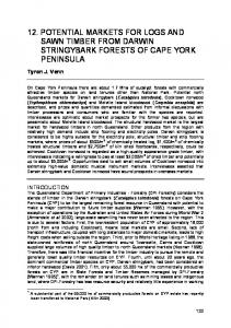
task complexity

individual capacity

performance Figure 1.1 Representation of the assessment of components of the relational complexity theory.

Figure 1.1 helps explain this situation further. Here individual performance is represented as a function of both the demands of the task and the processing capacity of the individual (single-headed arrows). However, performance is also the measure used to test the theory, and it is used to independently assess both the complexity manipulation and processing capacity (bold arrows). The logic of the argument needs to

5

be qualified. We cannot assess task complexity simply using performance because it is confounded with capacity to an unknown extent. Similarly, the assessment of capacity using performance is confounded with complexity, once again to an unknown extent. In fact Halford (1989, p. 126) has identified the same criticism in relation to capacity: “…when performance has been attributed to capacity, the term has often been used in a way that is synonymous with performance. The explanation is then completely circular; performance is a function of capacity, but performance is the only indicator of capacity.” Experimental manipulation can address these concerns up to a point and much of the empirical work to date has employed the experimental paradigm (Halford, Andrews, Dalton, Boag, & Zielinski, in press; Andrews & Halford, 1998, etc). By carefully manipulating the complexity of the task and the capacity of the individual (typically using age) while holding as many other factors as possible constant, some assessment of validity can be achieved by comparing aggregated performance across groups of individuals and/or sets of items (Andrews & Halford, in press). So while the assessment of complexity and capacity uses the same measure (i.e., performance), it is obtained under stringent manipulation and with the assumption that the influence of potentially confounding factors are distributed equally across individuals/items. As will be argued below, this approach has the potential to mask reliable variation that may turn out to (strongly) qualify the effect being tested. This is particularly relevant if some of that reliable variation is due to some interaction between complexity and capacity (Lohman & Ippel, 1993). Ideally, what is needed is a more independent way of testing the presence of a complexity effect that takes into consideration individual differences in performance (and capacity) as well as aggregated (or group) differences. This issue is central to the thesis and requires a brief diversion into more traditional measurement literature that will be expanded on further in later chapters.

1.3

Assessing Capacity and Complexity

Our understanding of human reasoning has developed through two distinct methodological measurement paradigms (Cronbach, 1957; Hunt, 1980; Lohman, 1989; Sternberg, 1994). The experimental or comparison of means (COM) approach has dominated the field of cognitive psychology and is pervasive in much of the traditional

6

memory and information processing research. Theory development and testing from this approach is achieved through creative experimental manipulation and control. Assessment of variations between task conditions on one or more outcome measures typically forms the basis of theory testing in this paradigm. Individual variations are typically controlled statistically (as is done in within-subjects ANOVA designs) or through random assignment (as in the standard between-subjects ANOVA designs). In either case, the emphasis of the comparison of means approach is on aggregated differences associated with the experimental manipulation. Therefore variations between individuals not associated with this manipulation are not of direct interest and are ultimately treated as noise. As mentioned previously, this has been the predominant approach used to test the relational complexity theory. In the correlational or individual differences approach that is considered to have been established by Charles Spearman (Sternberg, 1990; 1994), far greater emphases is placed on trying to account for reliable individual variation rather than averaged group differences. This approach effectively defines the psychometric tradition that has dominated the field of differential psychology (also called individual differences psychology). An alternative way of conceptualizing the modelling of task performance that also takes into consideration the potential for individual differences comes from some of the measurement models of Item Response Theory. For instance, Susan Embretson has had success in modelling the influence of various task components in mental rotation type tasks using parameters from Item Response Theory (Embretson, 1995a; Embretson, 1993). Multidimensional Latent Trait Models incorporate the influence of weighted task components directly into the parameters of the IRT model. The benefit of using IRT is that the interaction between items and individuals are modelled formally. An individual’s ability is modelled as a function of the items they have solved and the characteristics of the components that make up those items. Essentially, what this means is that we can take a process theory of task performance and model the influence of different task characteristics on the individual. Both the experimental and differential approaches have been instrumental in cognition research (Deary, 2001) and very similar (if not identical) tasks and measures have been employed under both paradigms. Unfortunately, not only does there appear to be a persistent reluctance to combine the methods and approaches from these two paradigms

7

in any formative way (with some notable exceptions as listed above), there is also an apparent resistance to theory integration. Lohman and Ippel (1993) suggest that this might be a function of incompatibilities in the methodologies used by the two approaches. In any case, this has resulted in two groups of researchers using essentially the same measures to assess the same cognitive processes, with little if any communication between them. A review of both the correlational and comparison of means approaches reveals each has much to offer in assessing the function of relational complexity. We identify two methods that may be useful in differentiating the effect of relational complexity from other factors that might contribute reliably to variation in task performance. The first approach uses an extension of the dual-task paradigm developed by Hunt and Lansman (1982; see also Lansman & Hunt, 1982) that includes aspects of the individual differences paradigm to overcome some of the reported limitations of dual-task assessment of processing capacity. The second uses an extended psychometric study to explore relational complexity in adult cognition and the way it covaries with a selection of core cognitive abilities.

1.4

Overview of the Thesis

To address the issues discussed above an attempt is made in Chapter 2 to map the development of the theory of relational complexity and its relationship with individual differences theories of human reasoning. This serves two purposes. Firstly, it provides a necessary review of the reasoning literature. More importantly, mapping the development of our understanding of human reasoning has the potential to explicate measurement and assessment issues that have arisen previously. The way these issues have been addressed will serve as the starting point in assessing the importance of relational complexity in adult cognition. Chapter 2 includes the specification of the theorems of the relational complexity theory that are applied to the analysis of two cognitive tasks in Chapters 3 and 4. Chapter 3 considers a relational complexity analysis of the knight-knave task, a high-level reasoning puzzle investigated by a number of researchers (Rips, 1989; Byrne & Handley, 1997; Schroyens, Schaeken, & d'Ydewalle, 1999). Chapter 4 reviews the development of the Latin Square Task. This task that was created for this research to specifically test the principles of relational complexity. The next three chapters form the experimental component of the thesis and synthesise the experimental and correlational approaches in conjunction with applications of the

8

Rasch measurement model to explore more completely the role of relational complexity. Chapter 5 applies the dual-task methodology to the Latin Square task. We use the easy-to-hard paradigm developed by Hunt and Lansman (1982) that relies almost exclusively on the individual differences approach. Chapters 6 explores the comparison of means evidence individually for three relational complexity tasks. We also explore the psychometric evidence for the measures of fluid intelligence (Gf), crystallized intelligence (Gc), and short-term memory (SAR). Chapter 7 considers the relationship between the relational complexity manipulations in the three tasks, and their relationship with the measures of broad cognitive abilities. If relational complexity is similar to complexity as it is defined in the psychometric tradition (Stankov, 2000; Stankov & Crawford, 1993) an a priori relationship between task performance and Gf can be specified as a function of relational complexity. Specifically, as the relational complexity of a task increases, the correlation between task performance and Gf should also increase monotonically. In practical terms this implies that as complexity increases, task performance better differentiates between individuals of differing general reasoning abilities (as Gf is defined). This pattern of correlations is not necessarily expected to hold for the Gc and SAR factors. This offers a means of testing whether processes of equal complexity across different tasks and domains form a consistent latent factor. Finally, Chapter 8 attempts to integrate the main issues addressed in each of the chapters as it relates to the role of relational complexity in adult reasoning.

CHAPTER TWO COGNITIVE COMPLEXITY AND RELATIONAL COMPLEXITY THEORY 2

Introduction

Cognitive psychology at its purest is ground in theories of process that attempt to provide a conceptualization of such things as attentional resources (e.g., Just & Carpenter, 1992), processing capacity (Halford et al., 1998a), and the functioning of memory (Baddeley, 1992, 1986; Humphreys, Wiles, & Dennis, 1994). The earliest attempts to measure cognitive capacity or span of attention revealed the presence of limits that seemed to be fluid and dependent on many factors (Wundt, 1896, cited in Chapman, 1989). The seminal work of Miller (1956) demonstrated that a quantitative dimension existed in the number of items that could be attended to at once. Miller introduced the concept of chunks as a way to explain how people overcome the apparent limitation in storage capacity. Current conceptualisations of capacity are still often drafted in terms of storage capacity (Cowan, 2000). However Halford et al. (1998a) and others (e.g., Oberauer, Suss, Schulze, Wilhelm, & Wittmann, 2000) make a clear structural distinction between the storage and processing functions of working memory. Whether storage capacity can subsume the processing capacity literature as Cowan (2000) implies, or whether processing capacity might subsume storage capacity (Halford, Phillips, & Wilson, 2000) is still open to further exploration. What we are concerned with here is processing capacity and like storage capacity, the construct is based on a conceptualisation of resources.

2.1

Resource Theory

Various models of capacity and resources have been proposed since Miller’s (1956) identification of a quantitative limit in processing. Kahneman (1973) depicted an undifferentiated model of processing capacity that contains a single "pool" of resources that can be allocated in a continuous fashion as task demands increase. While differential interference in dual-task studies that Kahneman’s model was unable to account for provided support for a multiple resource model (Norman & Bobrow, 1975; Wickens, 1980; 1984; 1991; Fisk, Derrick, & Schneider, 1986), the basic assumption of resource allocation has remained virtually intact (Halford, 1993).

10

Identification of dual-task deficits has been instrumental in the development of our current understanding of the resource concept (e.g., Halford, 1993; Maybery, Bain, & Halford, 1986; Navon, 1984). A dual-task deficit occurs when the performance on one or both tasks deteriorates when attempted together. This deterioration is typically provided as evidence for the tasks' dependence on limited resources from a pool common to both tasks (Kahneman, 1973; Norman & Bobrow, 1975; Navon & Gopher, 1979; 1980). However, Navon (1984) argues that such deficits in themselves are poor indicators that tasks compete for resources per se. He suggests that in most cases dualtask deficits can be explained equally well and more parsimoniously without introducing the concept of resources and the additional baggage that the term entails (see below). For instance, Navon and Miller (1987) have shown that interference effects can be accounted for by outcome-conflict; conflict produced between the outcome of the processing required for one task and the processing required for the other task1. Navon (1984) therefore believes that the legitimate use of resource theory is only as a metaphor for interference or trade-off that is not due to the scarcity of any mental commodity. In any case, Navon's work served to highlight fundamental weaknesses in the traditional dual-task approach that needed to be addressed. Damos (1991b) and Wickens (1991) discuss a series of experimental controls and guidelines that can be used in the application of the traditional dual-task methodologies to minimise interference and outcome conflict. Hunt and Lansman (1982; Lansman & Hunt, 1982) have a fundamentally different response to Navon’s (1984) concerns. They propose using the individual differences methodology to test for differences in resource capacity after partialling out the influence of interference. This procedure is known as the easy-to-hard paradigm. Although some researchers have questioned the practicality of meeting the easy-to-hard assumptions (e.g., Stankov, 1987), the results of research using this approach has been interpreted to support the tenets of resource theory (Halford, Maybery, & Bain, 1986; Halford, 1989, 1993; Foley & Berch, 1997). Just and Carpenter (1992) use the conceptualisation of resources to define the functionality of working memory as it corresponds to the central executive component of Baddeley’s memory model (1986). They perceive working memory as a “…pool of

1

The Stroop effect can be considered an example of outcome-conflict in which the process of generating

a colour word interferes with another process that generates the name of an ink colour.

11

operational resources that perform the symbolic computations and thereby generate the intermediate and final products [of reasoning, problem solving, and language comprehension]” (Just & Carpenter, 1992, p. 122). This can be extended to describe (and predict) individual differences in performance as a function of the interplay between two factors; (i) strategy for allocation of the available resources to a task, and (ii) processing efficiency. The convergence of these and many other intuitive and empirical resource models (e.g., Polson & Friedman, 1988; Fisk et al., 1986; Boles & Law, 1998; Pashler, 1994) serve to support and consolidate resource theory as a conceptualization of the generic capacity construct. Wickens (1991) argues that although in isolation each piece of evidence for resources might be explained by a different concept, resource theory best accounts for all the processing capacity evidence together. We will review these issues in more detail in Chapter 5 where we discuss the application of the dual-task methodology to assess the differential processing demands of relational complexity.

2.1.1

Resources: A Cautionary Note

The sheer volume of research using the resource concept might be interpreted as construct validity, consistent with Wickens (1991) proposal. However, the broadness of its current use also brings into question whether the term is sufficiently well specified to be usefulness as a distinct construct (Oberauer & Kliegl, 2001). The resource concept was employed to assist with the development of models describing the limitations in memory and reasoning that were observed by the predecessors of our discipline. More recently it has been used to develop sophisticated computational models of cognitive performance (Just & Carpenter, 1992; Halford et al., 1998a). However talking about capacity or resources limitations seems inappropriate unless there is a clear indication of just what the resource entails – its internal structure and limits, and the limits of its application. Furthermore, if the resource concept is used to define a construct, then like all constructs its role in cognition should be placed in context with other postulated resources and constructs and with other accounts of working memory limitations such as interference and decay as suggested by Oberauer and Kliegl (2001). Unless this is done, the utility of the resource concept is as Navon (1984; Navon & Miller, 1987) suggests; as a metaphor for describing a poorly defined construct. We will also consider

12

these issues in our discussion of the empirical dual-task evidence presented in Chapter 5. 2.2

Relational Complexity Theory

The idea of relational reasoning is not new. Spearman’s (1923) conceptualization of intelligence implicated the eduction of relations and correlates – the ability to deal with complex relations, to understand relationships among stimuli, to comprehend the implications of these relations, and to formulate a conclusion. In current parlance, this is central to our understanding of Fluid Intelligence (Carroll, 1993). With the availability of sophisticated neural imaging technology, relational reasoning is also being used to explain the neurological correlates of executive function. Recent research has implicated the anterior dorsolateral prefrontal cortex in relational processing (Kroger et al., in press; Waltz et al., 1999). Waltz et al. (1999, p123) argue, “…relational reasoning appears critical for all tasks identified with executive processing and fluid intelligence”. As we hope to demonstrate, Halford and his colleagues have achieved a formalism detailing how reasoning is influenced by the relational structure of the task (Halford & Wilson, 1980; Halford et al., 1994; Halford et al., 1998a; Andrews & Halford, in press). The original purpose of the relational complexity theory was to provide a foundation from which to explore the developmental nature of processing capacity and its limitations (Halford, 1993). In the following sections we explore the specification of the theory and the implications for assessing the function of relational reasoning in adult cognition.

2.2.1

Specification of Relational Complexity

The concept of relational reasoning can be derived from the following premises: 1. Deduction entails processing relations between entities specific to the task or that are recalled from memory 2. Processing internally represented relations generates non-trivial cognitive demand 3. The complexity of the internally represented relation can be used to quantify the characteristics of the processes used in performing the task – this is relational complexity

13

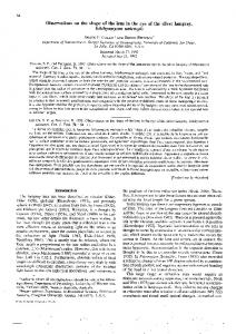
4. Further, processing capacity is a function of the relational complexity of the representations that an individual can process and therefore can be quantified using the same metric From this reasoning, there are essentially two axioms that form the basis of the relational complexity theory. We will consider the elaborations and implications of these axioms. Axiom 1: Complexity of a cognitive process: is the number of interacting variables that must be represented in parallel to implement that process (Halford et al., 1998a, p. 805). Axiom 2: Processing complexity of a task: is the number of interacting variables that must be represented in parallel to perform the most complex process involved in the task, using the least demanding strategy available to humans for that task (Halford et al., 1998a, p. 805). The formalisation of the relational complexity metric follows directly from these axioms. Relational complexity is considered to correspond to the arity or number of arguments of a relation. Unary relations have a single argument as in class membership, DOG(Fido). Binary relations have two arguments as in LARGER-THAN(elephant, mouse). Ternary relations have three arguments as in ADDITION(2,3,5) and quaternary relations have four arguments. Halford et al. (1998a) suggest that the upper limits of adult cognition tends to be at the quaternary level although under optimal circumstance quinary level processing may be possible. In general, the complexity of a relation, R(a, b, … , n), is determined by its arity, n. Each argument (a, b, … , n) is a source of variation in that it can be instantiated in more than one way under the condition that the relation is true (or at least perceived to be true). So for example, the binary operation of addition (e.g., 2 + 3 = 5) is a binding of three variables (2, 3, and 5), and is a ternary relation. The LARGER-THAN relation requires two arguments to be appropriately instantiated and is therefore a binary relation (see Figure 2.1).

14

LARGER-THAN (elephant, mouse) R (a, b,… n) Symbol for relation

RC = n No. of arguments

Figure 2.1. Representation of relations based on Halford et al. (1998a).

2.2.2

Chunking and Segmentation

One of the most interesting features of the relational complexity theory is the application of the complexity metric to characterise both features of the task and the processing capacity of the individual. That is, the implications of point 4 in section 2.2.1 above, is that the relational complexity of the most complex relation that can be processed can be used to quantify the limits of processing capacity – a characteristic of the individual. Much of the evidence for the relational complexity theory exploits this foundation. Given processing capacity limitations do constrain the amount of information that can be represented in parallel, an individual needs to be able to work within these limits. Relational complexity theory proposes that cognitive demand can be reduced through the processes of conceptual chunking and segmentation. Conceptual chunking is the recoding of a relation into a lower dimensional concept. For instance, velocity can be considered as a function of distance and time (velocity = distance/time), and in this form it entails a ternary relation which might be represented as either, RATIO(distance, time, velocity), or equivalently, RATIO(distance, time) → velocity (“ratio of distance to time implies velocity”). However, it can also be considered as a unary relation, such as VELOCITY(60km/hr). Conceptual chunking reduces processing demand, but at the cost that relations between chunked variables become inaccessible. While we think of speed as a unary relation, questions about time and distance cannot be considered. Segmentation entails reducing problems with many arguments into a series of lower dimensional processes that are solved in series. Relations are only defined between variables that are in the same segment (i.e., step) and relations between variables in different segments are inaccessible (Halford et al., 1998a).

15

2.2.3

Relational Complexity Theorems

Through the second axiom and the principles of chunking and segmentation, the theory is capable of modelling higher-level reasoning tasks that entail the representation and integration of more than one process for successful performance. Relational complexity of a task defined in this way captures the peak cognitive requirements of the task as a whole (Halford et al., 1998a). This conceptualisation has been used to broaden our understanding of dynamic situations such as air-traffic control (Boag, Neal, Halford, & Goodwin, 2000) in which task complexity varies across time. The issue of chunking and segmentation introduces three further theorems of the relational complexity theory: Theorem 1. Relational complexity is defined as the minimum dimensionality to which a representation can be reduced without the loss of information necessary for solution. This is referred to as the effective relational complexity. An example of this is outlined below, where the four arguments of mathematical proportion (a/b=c/d) are segmented into a number of ternary and binary relations that are solved in series. Theorem 2. Task complexity is defined as the effective relational complexity of the most complex process entailed in the task. This is a natural extension of Axiom 2 as applied to the first theorem. The effective relational complexity of the three processing steps required for mathematical proportion is ternary since this is the minimum dimensionality to which mathematical proportion can be reduced. Theorem 3. Arguments cannot be chunked or segmented if relations between them must be used in making the current decision. A corollary of Theorem 3 is the common arguments principle: Where two predicates (i.e., relations) have the same argument, and where they function as a unit for the current process, the predicates can be chunked.

16

Note: Theorem 3 is really an instantiation of Theorem 1 but is included separately because of its centrality in relational complexity analyses. An example of Theorem 3 is also provided above in the case of velocity. Further examples are provided in the analyses of the knight-knave task and the Latin Square Task in Chapters 3 and 4, respectively. Together the axioms of relational complexity theory and the chunking and segmentation principles form the foundations of the Method for Analysis of Relational Complexity (MARC).

2.2.4

Representation of Relations: A Comment on Notation

It is necessary to introduce some additional notation that will be used in the relational complexity analyses in subsequent chapters. An elaboration of the Halford et al. (1998a) notation makes it possible to represent higher-order relations that have one or more relations as arguments. Consider the relation, R(a, S(b, c), d). R is a higher-order relation defined by a, d, and the embedded binary relation, S(b, c). If the arguments of S do not need to be considered separately to make the current decision, then the relation can be chunked as a single argument of R (see Theorem 3). We represent chunking by underlining the elements that form the chunk. Therefore R would be represented by three underlined arguments and takes the form of a ternary relation: R(a, S(b, c), d,). The arguments a and d are also underlined as they are considered as chunks consisting of a single argument. An example of the analysis of embedded relations in the knightknave and Latin Square task is provided in the analysis of Chapters 3 and 4 respectively.

2.2.5

Evidence for Relational Complexity

The relational complexity metric receives empirical support from close to half a century of research in cognitive development. It is of course important that a theory be predictive and well as postdictive, and we will see that while the typical measures are variously sensitive to external factors, the relationship between the actual measure used to validate the complexity manipulation and other factors that influence task performance needs special consideration. It is important to recall that the relational complexity theory was developed to explain processing capacity limitations in relation

17

to cognitive development and the evidence for the theory has therefore predominantly been developmental in nature. In the following sections we summarise the empirical and theoretical support offered by i) the age of attainment literature, ii) secondary task performance in dual-task studies, iii) the neurological correlates research, and iv) perceived or subjective workload ratings. It is important to consider these factors even though adult cognition is of interest in the current research. Issues surrounding the developmental evidence may provide insights into problems that might be encountered in testing the theory with adults. Similarly, the application of the theory to an adult population might assist in clarifying some of the developmental evidence.

2.2.5.1 Age of attainment and knowledge acquisition. Age of attainment is the primary evidence used by Halford and his colleagues to support their conceptualisation of processing capacity limitations as a function of relational complexity (e.g., Halford & Dalton, 1995; Halford et al., 1986; Halford, Bain, & Maybery, 1984a). They argue that while their approach is not a true stage model in the Piagatian sense, there is a correspondence between the Piagatian stages and the age of attainment on tasks that have similar relational structure. The argument runs as follows: If children of a given age are capable of processing a task entailing ternary relations (say), then they should also be able to perform at similar levels in tasks from other domains that require ternary level processing (given sufficient instruction and knowledge of the new task domain). The converse is of course a little more difficult to verify logically (i.e., that children unable to process ternary relations in one domain will not be able to process ternary relations in another domain)2. The age of attainment criterion is an accepted criterion in the developmental literature and has been used to assess the influence of relational complexity in an increasing number of traditional developmental tasks such as transitive inference, class inclusion, and hierarchical classification (Halford et al., 1986; Andrews & Halford, 1998; Halford, Andrews, & Jensen, in press; Andrews & Halford, in press). This research demonstrates that different tasks which entail ternary relations have similar ages of attainment.

2

Fallacy of denying the antecedent: If A then B, not A → not B

18

Another task in which age of attainment has been used to test the relational complexity theory is the balance beam task (Halford, Andrews, Dalton et al., in press) discussed in Section 2.2.6.1. This task is typically difficult for children below about 11 years (Halford, 1993; Halford et al., 1998a). Even adults rarely use the appropriate crossproduct algorithm to take into consideration the combined influence of weight and distance from the fulcrum. They often revert to processing less efficient and error prone relations that are of a lower complexity. Together this suggests that knowledge is also a significant source of difficulty. In terms of age of attainment, Halford, Andrews, Dalton et al. (in press) demonstrated that binary components of the balance beam task but not ternary components were available to children of two years. Five to six year old children were capable of processing the ternary components. This is consistent with the predictions of the relational complexity theory. Relational Complexity, Age of Attainment, and Capacity: Not all researchers recognise age of attainment as suitable evidence to validate relational complexity as a metric for cognitive development. Goswami (1998) suggests that a key problem with the Halford et al. (1998a) analyses is that there is no independent evidence of whether a child is solving tasks on the basis of relational mappings. This criticism of independence could be targeted at many cognitive process theories, but certainly, it is important to have more than one source of evidence to substantiate the theory. As was indicated in Chapter 1, a primary focus of this thesis is to provide independent evidence for the influence of relational complexity on reasoning. Gentner and Rattermann (1998) argue that at least in terms of the development of analogical abilities, it is difficult to differentiate maturational effects from a knowledge-based account of performance. Rather than a change in processing capacity, Gentner and Rattermann question whether it is a change in the knowledge of the relations entailed (through the learning of relational labels) that accounts for age of attainment effects from infancy to adulthood. As discussed in Section 2.2.6.1, these issues are also relevant to the more advance levels of the balance beam task. Simply demonstrating that tasks in which the effect of relational complexity have been observed on performance can account for a very large proportion of the age related variation in other tasks in which the influence of relational complexity has been reported (Halford, Andrews, & Jensen, in press; Halford, Andrews, Dalton et al., in press; Andrews & Halford, in press), does not in itself resolve the issue of alternative explanations. It only tells us unambiguously that chronological

19

development is associated with improved performance on relationally complex tasks. It does not differentiate between capacity and other factors (e.g., knowledge) as the primary cause of this improvement. In adult cognition the concerns with the age of attainment criterion is less pressing and the influence of knowledge becomes much more prominent. Related to this less directly is the work of Salthouse (1985; Salthouse, 1988) who report findings that performance differences between young and old subjects becomes greater as the complexity of the task increases. In a sophisticated structural equation model, Stankov (1994) demonstrated that this effect, referred to as the Complexity Effect Phenomena, is actually an epiphenomena in that it is predominantly a function of the well reported age related decline in Gf during late adulthood. In fact age per se did not contribute any additional variance beyond what Gf accounted for. This finding has interesting implications for testing the relational complexity effect in children. It seems to be the case that relational reasoning is central to fluid intelligence (we will argue this point more strongly after presenting empirical evidence collected in this project). If we are permitted to conceptualise fluid intelligence as the capacity to process relationally complex tasks3, then the increasing nature of Gf in the first few years of life (Horn, 1988) might allow for an interpretation of the age of attainment evidence that is less entwined with acquired knowledge (i.e., given the distinction between Gf and Gc – see Section 2.3 below). Disambiguating Capacity, Knowledge, and Relational Complexity: Sweller (1998) expresses similar concerns about the influence of knowledge on performance and more importantly how the relational complexity theory is capable of dealing with individual differences in chunking and segmentation (this issue is raised in reference to mathematical proportion and the balance beam task in Section 2.2.6.1). That is, to what extent does different segmentation strategies (either taught or acquired) change the effective relational complexity of a task and more importantly, how can differential use of strategies be identified? This is a legitimate concern and one taken very seriously in the application of MARC in the tasks that are employed here. Halford et al. (1998a) are

3

This is against the recommendation of Stankov (1994) who prefers to conceptualise this statement as

only a figure of speech.

20

correct in stating that difficulty in establishing a reliable process theory of the strategies (or “schemas” in Sweller’s parlance) on which the relational complexity analysis can be imposed, does not invalidate the theory. It is also true that cognitive psychology, if nothing else, has been very successful in developing the tools for process/component analyses in a large number of tasks ranging from syllogistic/propositional reasoning (Sternberg, 1977; Maybery, 1987; Johnson-Laird, Byrne, & Schaeken, 1992) to mental rotation tasks (Shepard & Metzler, 1971; Pellegrino & Kail, 1982; Embretson, 1993), and even more complex tasks like the Raven’s progressive matrices (Carpenter, Just, & Shell, 1990). However, the ability to accurately identify strategies does cause some concern about the practical utility of the application of relational complexity theory to less well-known domains, in tasks that entail multiple correct solution strategies, or in tasks that come from more dynamic environments in which the complexity of stimuli changes over time. This is an important issue and one that we will return to in the final chapter.

2.2.5.2 Dual-task evidence for relational complexity. It is not surprising that given the emphasis that Halford et al. (1998a) put on processing capacity and resource theory, a second type of empirical support for the relational complexity theory is provided by dual-task studies. Maybery et al. (1986; see also Halford et al., 1986) investigated binary and ternary processing load in the N-term series task via a probe reaction time measure. With memory load and number of terms controlled, significantly longer reaction times were observed at the point where the three terms had to be integrated in parallel (to make a transitive inference, i.e., a ternary relation) than when three terms could be integrated in series (a matched verification task, i.e., a binary relation). The dual-task approach has also been used independently of Halford’ laboratory to explore hierarchical reasoning consistent with the predictions of relational complexity theory (Foley, 1997; Foley & Berch, 1997). We will explore this in more detail in Chapter 5.

2.2.5.3 Neural imaging evidence. Additional evidence that processing complexity is a function of relational complexity comes from research exploring neurological correlates of reasoning. Kroger et al. (in

21

press) and Waltz et al. (1999) have implicated the anterior dorsolateral prefrontal cortex in relational processing. Kroger et al. manipulated five levels of complexity that are similar to manipulations of relational complexity4 and four levels of item difficulty in tasks resembling the Raven’s progressive matrices. The data was supportive of increasing neural activity as complexity increases. Waltz et al. (1999, p123) argue, “relational reasoning appears critical for all tasks identified with executive processing and fluid intelligence”. Complementary to this is the work of Gevins and Smith (2000), who demonstrated that individual differences in broad cognitive abilities are related to differential cortical activity as a function of complexity during solution of the N-back task. There is also some preliminary indications from Halford’s laboratory that different levels of the N-back task correspond to differences in relational complexity (Halford & Zielinski, in preparation).

2.2.5.4 Subjective ratings and other evidence. Another test of the relational complexity theory is provided by Andrews and Halford (1995; Andrews, 1997) who have considered ratings of perceived workload in the comprehension of embedded sentences (this task is used in Chapters 6 and 7, and the details are discussed there). They have demonstrated high correlations (r > .80) between subjects perceived complexity of the task and manipulations of relational complexity within the task. Subjective ratings of cognitive demand have also been used to assess the relational complexity analysis of static air-traffic control scenarios (Boag et al., 2000). As a final point of support it is useful to consider the position of the relational complexity model in terms of other theories of cognitive process. Halford et al. (1998a) argue that the relational complexity approach provides a more succinct account of performance in the Tower of Hanoi task (Loveday, 1995) than the traditional embedded subgoals (i.e., steps) procedure used by Just, Carpenter and Hemphill (1996; see also Carpenter et al., 1990). Further empirical testing of relational complexity in the Tower of Hanoi is currently in progress in Halford's laboratory. Evidence of the ability of the 4

The conceptualisation of relational reasoning by Waltz (1999) and Kroger (in press) use the number of

relations to be processed as a metric of complexity rather than the number of arguments in the relation per se, and therefore is somewhat different to that specified by Halford et al. (1998a).

22

relational complexity theory to subsume aspects of mental models (Johnson-Laird et al., 1992) and deduction rule (Rips, 1994; Braine, 1990) theories of cognition are considered in Chapter 3.

2.2.6

Unresolved Issues

The relational complexity theory is sufficiently well specified to be applied independent of task domain and as a result is capable of making strong predictions about processing capacity. As we have seen, many of these predictions have empirical and theoretical support of varying degrees from (i) the age of attainment literature, (ii) secondary task performance in dual-task studies, (iii) the neurological correlates research and (iv); perceived or subjective workload ratings, and many of these entail some comparison of simple error or reaction time data. It is clear that the role of alternative explanations in each of these measures varies and for reasons that we have alluded to already (Chapter 1), external validation of the relational complexity metric requires assessment techniques that are more independent of confounding factors that might influence performance. That is, although the specifications of the relational complexity theory are detailed enough to allow various predictions to be made, the assessment of these predictions are open to a large number of potentially confounding factors. In addition to those we have already mentioned, other factors that might influence performance on cognitive tasks somewhat independent of the available processing resources might include differential rates of schema acquisition (Kanfer & Ackerman, 1989) and intratask learning, individual differences in cognitive variables such as spatial and verbal abilities (e.g., Lohman & Kyllonen, 1983), and individual differences in affective variables such as impulsivity, persistence, confidence, and motivation (e.g., Stankov, 2000; Kanfer & Ackerman, 1989; Embretson & Prenovost, 2000). Given these potentially confounding factors, the problem for a theory of relational complexity becomes how to isolate the effect of a complexity manipulation in measures of performance from these other factors.

2.2.6.1 Conflicting results using segmentation and chunking. While the above evidence shows general and converging evidence for the influence of relational complexity on processing capacity and development, the application of the

23

theory to specific tasks analysis has shown to result in some inconsistencies. In particular, some apparent inconsistencies in the application of segmentation and chunking principles would benefit from further clarification. The theory relies heavily on these principles and it is important to make a distinction between what is possible within the limits of the theory as it stands and issues that are yet to be resolved. Segmentation and chunking can influence the relational complexity classification of a task. Halford et al. (1998a, p. 809) cite mathematical proportion (a/b = c/d) as an exemplar of a quaternary relation. The thesis presented by Halford et al. is that a/b = c/d entails four terms (a, b, c, d) that are constrained by the proportion relation and is therefore a quaternary process. This means that given any three terms plus the knowledge that proportion is entailed, it is possible to predict the remaining term (case 1: proportion(a,b,c,?)). Alternatively, if all four terms are provided, it is possible to determine whether proportion follows (case 2: ?(a,b,c,d)). Although the prima facie’ complexity of proportion may be quaternary, when the influence of strategy through segmentation is considered, the effective relational complexity is ternary5. Halford et al. (1998a) argue that both case 1 and 2 require representation of a quaternary process for solution and therefore classify proportion as quaternary. However, they also state that a series of ternary processes (and some algebraic knowledge) are all that is needed to instantiate proportion in practice (Halford, Wilson, & Phillips, 1998b, p852). In applying the axioms and theorems of relational complexity theory, the classification of proportion should therefore be ternary. Another example of the same inconsistency is apparent in parts of the relational complexity analysis of the balance-beam task. Algorithmic performance on the balance beam task entails an application of a variant on mathematical proportion and has similarly been classified as quaternary (Halford, Andrews, Dalton et al., in press). To determine whether the beam will balance, the product of weight and distance on one side of the beam can be compared with the product of weight and distance on the other. This is referred to as the product rule entailing the concept of torque. That is, weightleft × distanceleft = weightright × distanceright, the complexity of which Halford, Andrews,

5

Pascual-Leone (1998) classifies the same problem as requiring six arguments, although his application

of the principles of relational complexity theory is not accurate

24

Dalton et al. represent as BALANCE-TORQUE(weightleft, distanceleft, weightright, distanceright). Once again, the authors correctly state that the task can be segmented into two ternary relations (and a binary comparison of the output of each) to determine proportion – or in the context of this task, balance. However, once again the argument presented by Halford, Andrews, Dalton et al. for a requirement of quaternary processing is not really convincing; “… while the most complex relation that has to be computed is ternary for both the addition and product rules, acquisition of the product rule might require representation of the quaternary relational torque rule (emphasis added)”6. An equally plausible interpretation of the relative difficulty in conceptualising the influence of weight and distance, is that the product rule requires an acquisition of knowledge of torque that is either not available or not easily accessible in that it is unlikely to have been proceduralised in the context of the balance beam task. Halford et al. (in press) did train subjects on the concepts of weight and distance but the possibility of the interaction between the two was not demonstrated. It could be argued that acquiring the torque schema unprompted is likely to take many more trials than what was presented. As a caveat it is important to note that the emphasis of the research was to demonstrate age related differences in the capacity to deal with binary and ternary relations and was not contingent on the exact classification of the product-rule. As such, the data provided as support for the study’s hypotheses is not compromised by the authors’ classification of the product rule. To address this inconsistency we need to consider more closely the principles of segmentation and chunking. Remember, the essence of relational complexity is that the relation constrains the possible values that the arguments can take; just as the particular instantiation of the arguments constrains possible relations (this idea is referred to in the principle of omni-directional access by Halford et al., 1998a, p817). Hence a relation cannot be decomposed if the variables interact, because interacting variables must be interpreted jointly. This is the case for all relations regardless of complexity level. So the question is, what constrains proportion from being decomposed from a quaternary relation? It is suggested by Halford et al. (1998b, p852) that to plan the implementation

6

The addition rule is referred to as a “buggy rule” since it entails the addition of the number of weights

and distance from the fulcrum in number of pegs

25

of the separate ternary processes entailed in mathematical proportion, “…or to understand why it is valid, the structure of proportion must be represented”. A similar argument is applied to the torque rule of the balance beam task (Halford, Andrews, Dalton et al., in press). Using this conceptualisation, both tasks remain quaternary even after segmentation to a series of ternary relations. This is a little awkward as it is inconsistent with the principle of effective relational complexity (Theorem 1) and has the potential to introduce substantial subjectivity and vagueness into complexity analyses. In any case, the relational complexity theory does not seem to be well equipped at this stage to model this type of pre-processing in a way that is independent of procedural knowledge (see comments by Sweller, 1998, that we raised earlier). That is, from the relational complexity framework it is very difficult to conceptualise the representation of implicit knowledge (e.g., proportion or torque) independent of the explicit solution strategy. In fact, the empirical data for the balance-beam task also suggests that knowledge is a significant source of difficulty. Halford, Andrews, Dalton et al. (in press) state that even adults have difficulty with the product rule. Given that Halford et al. (1998a) would argue that the majority of adults are capable of processing quaternary relations it would be reasonable to speculate that the additional difficulty observed is some function of knowledge. The proportion example is important because it demonstrates the necessity for a clear understanding of the available strategies in order to apply the principles of segmentation and chunking. We suspect this is particularly relevant in assessing the distinction between ternary and quaternary problems within the realm of adult cognition because strategies are likely to be much more influential than with children. The proportion example also highlights a possible looseness in the interpretation of the chunking and segmentation principles that could benefit from some further formalisation. The interpretation of the MARC approach that we adopt is therefore strictly in line with the formalism of Halford et al. (1998a). It is also more in line with process theorists such as Johnson-Laird who, while acknowledging implicit reasoning as a factor in performance, effectively model only explicit processes formally (e.g., Johnson-Laird & Byrne, 1991; Johnson-Laird et al., 1992). Strictly speaking, this is also the view of Halford and his associates: “The metric applies to explicitly represented relations… It does not apply to associations or automatic processes” (Halford, Andrews, & Jensen, in press, emphasis added). In Chapter 4 (Section 4.10.1), we discuss similar issues that arise in the

26

determination of segmentation and chunking in the Latin Square Task. In the following section we consider the conceptualisation of cognitive complexity from the individual differences approach.

2.3

Cognitive Complexity: A Psychometric Approach

We have already noted that Spearman (1923) referred to three qualitative principles of cognition. R. J. Sternberg (1977; 1984) summarises each of these as follows: Apprehension of experience: Encoding – the perception of a stimulus and the relation of it to the contents of long term memory Eduction of relations: Inference – the interrelation of two stimuli so as to understand their differences Eduction of correlates: Application – the applying of an inferred relation to a new domain Sternberg (1977; 1984) suggests that this demonstrates that although the discipline of cognitive psychology is considered by many to have emerged in the 1960’s from the behaviourist tradition, links can be traced back to Charles Spearman (Skinner, 1983, prefers to see the emergence as a "retreat"!). That is, Spearman (1923) who is traditionally considered the father of the psychometric movement, was in fact proposing a cognitive approach to cognitive abilities. This link between experimental and correlational approaches has been exploited by only a handful of researchers beginning with a call by Cronbach (1957) for an integration. Earl Hunt pursued the idea in the 1980’s (Hunt, 1980; Hunt & Lansman, 1982) using the easy-to-hard paradigm, a variation on the dual-task methodology. Kyllonen and Christal (1990) explored individual differences in reasoning ability as defined in the psychometric literature (e.g., Carroll, 1993) and its relation to working memory capacity based on Baddeley’s (1986) cognitive psychology definition. More recently, Susan Embretson has attempted to integrate the experimental and differential psychology using IRT (e.g., Embretson, 1993; Embretson, 1995b, 1995a). Our aim is to exploit this tenuous link between experimental and differential psychology further to explore the basis of the relational

27

complexity theory in adult cognition. We use the Gf-Gc theory of cognitive abilities as the foundation from which to explore the influence of individual differences.

2.3.1

Gf-Gc Theory

The ability to reason and process relations seems to be central to human functioning. According to Carroll (1993), the eduction of correlates and relations can be regarded as reflecting elementary reasoning abilities and as we have already alluded to, these abilities are typically considered a component of fluid intelligence. The original distinction between fluid and crystallized intelligence was proposed by Raymond B. Cattell in the late 1950’s (Cattell, 1957) and refined further in association with John L. Horn (see Horn & Cattell, 1966; Horn, 1968; Cattell, 1987, for reviews). Fluid intelligence (Gf) is clinically interpreted as a non-verbal or performance component of intelligence that is relatively insensitive to education and to some extent culture (at least in theory, arguable never in practice7). In marker tests such as the Raven’s progressive matrices, it entails the ability to induce relations and deal with novelty. In fact novelty of situation and strategy variations are considered an important component of many theories of intelligent behaviour (e.g., see Sternberg, 1984; 1985, for reviews). Crystallized Intelligence (Gc) on the other hand, is regarded as an indication of the effect of acculturation and education on cognitive abilities. It is “... a type of broad mental ability that develops through the ‘investment’ of general intelligence into learning through education and experience.” (Carroll, 1993, p. 599). The broadness of both Gf and Gc is reflected in the significant cross-loadings of first order factors on these higher order abilities. For instance, the first order sequential reasoning (RG) factor independently contributes to the identification of both Gf and Gc (Carroll, 1993). If we consider that transitive inference and categorical syllogism tasks typically load on the RG factor, then it becomes intuitively reasonable that significant higher order loadings would exist on both Gc and Gf. That is, performance on these types of tasks is likely to be facilitated by both verbal and non-verbal reasoning skills. The methodological consequence of this cross-loading effect is that it becomes important to use more than 7

It is important to note that the measurement of psychological constructs will always contain variation

due to individual differences in experience. Hence, while in theory Gf might be free of culture and education, it will never be so in practice.

28

one marker variable for each broad factor to avoid possible misidentification in factor scores8. In terms of the current project, we need to be especially sure that Gf and Gc are well identified in the data since, as we will see, they both have a role in validating the relational complexity theory. Short-term Apprehension and Retrieval (SAR) is another psychometric factor that is relevant in the current work. This factor can be considered as the psychometric equivalent to working memory, as identified by memory tasks in which individual differences have been observed. Carroll (1993) reports several studies in which this factor has been uniquely identified distinct from Gf and this is consistent with cognitive psychology's notion that processing and storage should be treated as somewhat separate systems (Halford et al., 2000; Cowan, 2000).

2.3.2

Psychometric Complexity

The issue of complexity has been pervasive throughout the psychometric movement. It is almost taken for granted that increases in task complexity are associated with increased demands on the information processing system (Larson, Merritt, & Williams, 1988; Pellegrino & Glaser, 1979; Stankov, 2000; Crawford, 1991). While Spearman's general factor (g) was proposed to account for positive manifold, Jensen (1987a) argues that the most undisputed fact about ‘g’ is that loadings of tasks on this factor are an increasing monotonic function of the tasks’ perceived complexity. Marshalek, Lohman, and Snow (1983, p. 108) argue that the “…actual correlation between a test and ‘g’ approximates the apparent complexity of its required operations”. Further, they propose that an understanding of complexity is essential to understanding intelligence. The association between complexity and "intelligence" can also be seen in Louis Guttman’s facet theory that describes the structure of human abilities using the radex model

8

A common although erroneous assumption made in many psychometric studies is that using only the

central marker of a factor is sufficient when correlating it with other tasks. The Raven’s matrices for instance, is considered central to defining Gf (e.g., Carpenter et al., 1990; Stankov, Boyle, & Cattell, 1995). However, all abilities that contribute to the definition of Gf are not necessarily assessed by this one test. Using only one marker to define a factor has the potential to change the nature of the factors that emerge. This practice should be avoided as it can lead to unexpected loadings with other factors and tasks.

29

(radical expansion of complexity) (see Snow, Kyllonen, & Marshalek, 1984; Most & Zeidner, 1995; Marshalek et al., 1983; and Stankov et al., 1995, for reviews). In this model, tasks of different cognitive complexity are arranged in a series of concentric circles such that more complex tasks that measure problem solving and higher-level mental processes like Raven’s progressive matrices are grouped at the centre. The domain specific and less complex tasks fall in the outer bands with sensory-type tasks at the periphery. By its very nature, this approach avoids the constraints of the Cartesian system of vectors in preference for a conceptualisation of the problem space using polar coordinates. As an independent confirmation, Snow et al. (1984) used multidimensional scaling techniques to classify the relationship between cognitive tasks along the lines of Guttman’s theory. While differences in the identification of specific cognitive abilities existed, the association between complexity and intelligence was consistent with Guttman’s conceptualisation. Cognitive complexity is manipulated rather than just observed in a more pragmatic approach provided by Stankov (2000). In this work, Stankov (2000, p. 123) adopts what he refers to as an eclectic approach to increasing the cognitive complexity of a task. He states that any manipulation that results in systematic changes in the factor loadings with Fluid Intelligence (Gf) will suffice as a complexity manipulation since the “ …empirical evidence is assumed to be the final arbiter”. This statistical criterion which we will refer to as the complexity-Gf effect, is based on the theoretical assumption that the factorial structure of intelligence is such that defining any one specific process to account for complexity reduces our understanding of what Gf is, a broad multi-faceted construct. In fact Stankov argues that too much emphasis has been placed on the process theories of cognitive psychology. Lohman (1994) tends to agree and states that the ambition of cognitive psychology in the 1970’s to rescue differential psychology from psychometrics by providing measures of basic information processing capabilities through decomposing individual differences, has resulted in weak and inconsistent correlations with traditional estimates of abilities. To some extent we agree with this observation, however we would like to point out an important distinction that needs to be made. Relational complexity theory is effectively domain independent – it is a theory about processing resources and task complexity and might more appropriately be conceptualised as a theory of process rather than a process theory in the componential sense typified by the work of R.J. Sternberg in the late 1970’s (Sternberg, 1977;

30

Pellegrino & Lyon, 1979). Having said this, the application of MARC does require a process theory of the strategies that are entailed. We will argue in Chapter 3, that the appropriateness of a relational complexity analysis is dependent on the success of the process theory on which it is based. The rationale for the psychometric conceptualisation of cognitive complexity, the complexity-Gf effect, is appealing. Performances on complex cognitive tasks entail understanding the relations among task stimuli, comprehension of the implications of these relations, and the formulation of a conclusion based on this processing. These are the characteristics that define fluid abilities (Carroll, 1993). It follows that if we increase the complexity of a task this should result in a concomitant increase in the demand placed on these fluid abilities. As Figure 2.2 indicates, this in turn should result in better discrimination between individuals of high and low Gf, and the pattern of monotonic increasing correlations between task performance and Gf (Stankov, 1994). We will demonstrate in our analyses that the relational complexity theory may provide a

Performance

more detailed specification and understanding of the facets of Gf.

high-Gf

low-Gf low

high

Cognitive Complexity Figure 2.2. The complexity-Gf effect: The hypothetical relationship between performance and Gf as function of cognitive complexity

2.3.3

Fluid Intelligence and Complexity: The Evidence

Although attempts have been made and a psychometric criterion identified, there is no global consensus in the psychometric literature on just what has to be done to satisfy an operational definition of complexity. Crawford (1991) has reviewed a number of approaches to defining complexity and has integrated the particularly interesting role of

31

strategy variation as an influence on complexity. The key idea as expressed by Sternberg (1985) is that novel tasks call for the greater involvement of strategic or metacomponential processes and are therefore closely related to measures of general intelligence. Hunt (1980) takes a consistent but slightly different perspective and argues that the tests in the periphery of the radex model described above, have low Gf loadings because they are very constrained and typically have a limited range of possible strategies. Therefore they tend to be more determined by mechanistic information processing functions (Crawford, 1991) rather than the executive/control functions that are typically associated with Gf tasks. Stankov and his associates (e.g., Stankov, 1988; Spilsbury, Stankov, & Roberts, 1990; Stankov, 2000; Stankov & Crawford, 1993; Stankov & Raykov, 1995) have manipulated complexity using a variety of methods in both dual- and single-task designs and we consider examples related to each of these in turn.

2.3.3.1 Dual-task evidence. In what is referred to as a competing task paradigm, two independent cognitive tasks are presented simultaneously with response priority order varied post-presentation (i.e., subjects are told which of the two tasks to respond to first after the presentation). The complexity manipulation is the combination of the two component tasks. The competing task as a manipulation of complexity is supported by an increase in correlations with Gf (Fogarty & Stankov, 1982; Stankov, 1987; Roberts, Beh, & Stankov, 1988). However, the presence of the complexity-Gf effect in the competing task paradigm is qualified. Firstly, Fogarty and Stankov (1982) report that the complexity effect is negated when the correlation between the single tests are themselves very high9. Second, Fogarty and Stankov (1988) found that competing tasks have higher Gf loadings than their single task counterparts only when the latter have relatively low ‘g’ loadings (the converse is particularly interesting; when single tasks have high ‘g’ loadings, the competing task tends not to be highly correlated with ‘g’). Finally, a difficulty effect (decrement in aggregated performance) is not always a necessary consequence of a complexity manipulation. Stankov (1988) reports a

9

It may be that the correlation between single component tasks is high when they both draw on the same

processes or resources and that this might contribute to the reduction in correlations with ‘g’.

32

complexity effect in which there is no change in mean performance from the single task to the competing task, but the expected increase in correlations with Gf was observed (the tasks were a tonal memory test and an embedded figures test). In the same study, an experiment is reported in which arithmetic mean performance in a multi-element counting task actually increased from the single condition (sequential presentation of two categories) to the competing condition (simultaneous presentation of two categories). Stankov (1988) suggests that both these results indicate that processing capacity limitations per se cannot account for individual differences in the tasks used without some multiple resource type theory. It might also be the case that under more difficult conditions, individuals will invest more effort to recruit more resources to not only maintain, but increase overall performance (Kanfer & Ackerman, 1989). The implication of this on the utility of resource theory and the investigation of dual-task deficits is considered in Chapter 5. In any case, Stankov’s example is significant to the extent that with appropriate tasks, such cases are rare (Stankov & Raykov, 1995). The potential however is real, and this supports our emphasis on the need to use an external criterion for complexity other then mean performance data.

2.3.3.2 Complexity and single tasks. Mixed results have also been achieved under the single task approach. Spilsbury, Stankov, and Roberts (1990) used a manipulation of premise presentation order of the 4-term series task (that entails transitive reasoning) as the complexity variable. There was no evidence to suggest that the manipulation resulted in changes in correlations although changes in item difficulty (and efficiency) were observed. This implies that the manipulation was one of difficulty and not complexity. Similar results to Spilsbury et al. (1990) have been observed in data from Halford's laboratory with variations of the Nterm series task (Birney, 1999). Such results are consistent with the relational complexity theory since manipulations of the number of premises and the presentation order does not change the inherent dimensionality or complexity of transitive reasoning required which is essentially ternary (Halford, 1993). Using a complexity manipulation that on the surface at least is more in line with the Halford et al. (1998a) conceptualization, Stankov and Crawford (1993) have successfully demonstrated a reliable and increasing monotonic relationship between

33

performance and Gf in two experimental tasks. The Triplet Numbers Test required subjects to validate increasingly complex rules against a randomly generated sequences of three digits. For instance, given the number triplet "3 6 4", subjects might be asked to verify whether " …the second digit is the largest and the third digit is the smallest". The manipulation of complexity involved increasing the number of elements in the rule. The second experimental task used by Stankov and Crawford (1993) was the Swaps Test. This task required subjects to rearrange a letter triplet following increasingly complex instructions. For instance, given the letter triplet, "J K L", subjects are asked to specify the resulting order after the position of elements had been hypothetically swapped. The complexity manipulation in this test was the number of swaps to be made. Both these tasks are to be included in the current series of studies and are discussed in more detail by Stankov and Crawford (1993). It is interesting to note that an additional measure of short-term memory employed by Stankov and Crawford (the forward and backward digit span tests) did not show the same increasing monotonic correlations with the complexity manipulation as Gf did. From these findings Stankov and Crawford (1993, p. 106) suggest that the main “ingredient” of complexity is the "…number of elements and relations that have to be dealt with while a person tries to solve a problem."

2.3.3.3 Relational complexity and Gf-Gc theory. The complexity-Gf effect does not receive unanimous support. Researchers such as Schweizer (1998), who reports a reversed complexity-Gf effect10 suggests that the strength of the prediction is lessened by the variety of meanings attributed to complexity. It is also tempting to over-emphasise the obvious similarity in the role of relations and elements that Stankov talks about, with those specified in the relational complexity theory. There is no theoretical justification at this stage to expect that Stankov and Crawford’s (1993) conceptualisation of “relations” is fundamentally different from that specified in the relational complexity theory, there is also no evidence to suggest otherwise. Yet, it is encouraging that the two different approaches provided by Halford and Stankov independently should arrive at compatible

10

By reversed, we mean that the correlations between performance and Gf decreased as the number of

operations to be processed (the manipulation of complexity) was increased (Schweizer, 1998).

34

conclusions. Relational complexity theory incorporates the conceptual distinction between the Gf and Gc factors in what might be a natural way. It specifies that the cognitive load on resources is generated by processing relations relatively independent of content and domain, and that education can mediate the efficiency in which resources are applied (e.g., through appropriate segmentation) but does not influence the individual's processing capacity. It seems clear that an association between the theoretical characteristics of processing capacity and fluid intelligence exists (Hunt, 1987; Kyllonen & Christal, 1990). Relational complexity theory is ground firmly in a theory of process whose psychometric properties are not well known. If the relational complexity manipulation is consistent with the notion of cognitive complexity in the psychometric tradition, then we should observe a similar pattern of monotonic increasing correlations with Gf indicative of the complexity-Gf effect. More importantly, the complexity-Gf effect serves as an external criterion for the relational complexity manipulation that is less dependent on the task being manipulated.

2.3.4

Some Final Methodological Issues

The unifying goal of this project is to test the relational complexity theory using measures independent of the task whose relational complexity is being manipulated. We have argued that this entails bringing together methodologies from experimental and differential psychology. Although there is recognition that a merger of these areas is necessary (Hunt, 1980; Kyllonen & Christal, 1990; Deary, 2001), history suggests that such a venture has failed to be fully realised. Lohman and Ippel (1993) have argued that the psychometric approach to cognition, despite the very best of intentions from the outset, has been disappointing in its ability to provide a clear conception of what a process underlying broad cognitive factors such as Gf might entail. They argue that the information processing approach central to cognitive psychology provides not so much a model, but a general framework to advance this understanding. Deary (2001) suggests that the merging point will be the coming together of working memory and intelligence differences, and that this relies on a more resolute attempt to develop validated cognitive architectures that have isolable and testable constructs and processes than has

35

so far been achieved. As such, the weight of responsibility is placed with experimental psychology in general and cognitive psychology in particular. Lohman and Ippel (1993, p. 68) take a slightly different perspective. They suggest that “… the generally accepted idea of test theory as applied statistics seems to have precluded the development of a structural theory of measurement needed for the measurement of processes”. Therefore, according to Lohman and Ippel, at least some of the reasons for the relative failure of a merger, has to do with the fundamental differences and incompatibilities of the two approaches used. For instance, the methodologies of factorial theories of intelligence assume that the underlying latent constructs are relatively stable characteristics of the individual that remain constant during testing – the focus is on between-individual differences. In research directed at describing the processes by which a subjects arrives at the answer to a problem, experimental psychologist arrange observation conditions to reveal differences in responses. The focus is on within-individual differences (although typically at a group level). The Raven’s progressive matrices is an interesting task that might serve to clarify the distinction being made by Lohman and Ippel (1993). Consider a differential psychologists use of the progressive matrices test. Performance will be considered to reflect individual ability to deal with novelty and induce patterns and relationships – to reflect individual differences in latent fluid abilities. An experimentalist might use the task for somewhat different purposes. They might focus on what changes in the individual as a function of working through the process of solving a series of matrices items. That is, to what extent are patterns discovered, relations induced, and strategies developed. The knowledge base that the individual uses to work through the test of 30 or 40 items does not remain static. It changes based on the experiences of each successive item; processing is dynamic, non-linear, and fluid. Consistent with Lohman and Ippel, we therefore believe that the merger of the experimental and differential perspectives on cognition will come through an investigation of individual differences in strategy that also differ in process. We will return to this idea in the discussion of Chapter 8. For now we return to the relational complexity theory and consider the current state of our predictions.

36

2.4

The Experimental Approach

We can now specify Axiom 3 to complete the foundation that will be used to assess the characteristics of the relational complexity metric. The full set is as follows: Axiom 1: Complexity of a cognitive process: is the number of interacting variables that must be represented in parallel to implement that process (Halford et al., 1998a, p. 805). Axiom 2: Processing complexity of a task: is the number of interacting variables that must be represented in parallel to perform the most complex process involved in the task, using the least demanding strategy available to humans for that task (Halford et al., 1998a, p. 805). Axiom 3: Complexity-Gf effect: Factor loadings on fluid intelligence are an increasing monotonic function of a tasks psychometric complexity.

The predictions to be outlined below demonstrate what we believe is a close conceptual relationship between the cognitive and psychometric approaches. The broad predictions to be explored by each study are then summarised.

2.4.1

Predictions

2.4.1.1 Aggregated performance: Comparison of means. From Axiom 1, we can predict that manipulations of relational complexity should incur resource costs that are reflected in the difficulty of a task. The Comparison of Means approach can be used to test for a relational complexity effect generated by a manipulation of a tasks relational structure. More complex tasks should have a smaller proportion of correct responses and all else equal, a tendency for longer response times11. From a psychological perspective this is a “weak condition” in that it is a sufficient but not a necessary condition to substantiate a relational complexity 11

This is a contentious issues and one raised by a reviewer of Birney and Halford (in press). We will

return to this issue in Chapter 7, Section 7.5.5.

37

manipulation (Spilsbury et al., 1990). The comparison of means approach assumes that memory and education are controlled in the design of the items or through careful selection of subjects (e.g., using age as a covariate), it cannot be used alone to control statistically for potentially confounding factors. There is also the problem of aggregating reliable or systematic within-subject variability in considering composite scores (Lohman & Ippel, 1993) and group/condition differences (Chapter 1).

2.4.1.2 Easy-to-hard correlations. One of the methods that we use is the easy-to-hard paradigm developed by Hunt and Lansman (1982) that relies almost exclusively on the individual differences approach. The easy-to-hard paradigm follows the dual-task approach to assessing processing capacity limitations. Subjects are given a secondary task alone and concurrently while solving an easy version of the primary task. Performance on the hard version of the primary task attempted alone is also assessed. The measure of processing capacity is the partial correlation between the secondary task (performed in conjunction with the easy primary task) and the hard primary task (performed alone). Removing common variation between the hard and easy primary task performed alone, and between the hard primary task and the secondary task performed alone, results in a relatively clean measure of variation due to resource limitations (Halford, 1989, 1993). This technique removes variance that the tasks might share that is not associated with resource limitations and overcomes the dual-task issue of conflict raised by Navon (1984). Since the hard primary task is never performed in a dual-task situation, variance that is shared with it and the secondary task cannot be associated with one task interfering with the other. Assuming primary task performance is maintained, the interpretation of a significant partial correlation is that performance on the secondary task is sensitive to individual differences in available resources. That is, it can serve as a measure of processing capacity and is considered in Chapter 5.

2.4.1.3 Controlling for confounding factors. Using the individual differences approach and the Gf-Gc theory of cognitive abilities the assessment of relational complexity in reasoning can be refined and its function further explored. In the study outlined in Chapters 6 and 7, three broad cognitive factors

38

are assessed – fluid intelligence (Gf), crystallized intelligence (Gc), and short-term apprehension and retrieval (SAR). Gc and SAR can be thought of as corresponding to the effect of education (and experience) and short-term memory respectively. Axiom 1 also implies that memory storage requirements do not influence relational complexity of the task per se. That is, while the limits of storage and processing capacity are similar in magnitude at about 4 elements in each (Cowan, 2000; Halford et al., 1998a), a conceptual distinction between the two is frequently made (Moray, 1967; Baddeley, 1996; Halford et al., 1984a; Maybery et al., 1986) even though there is some continuing debate over whether one of the systems can subsume the other (Cowan, 2000; Halford et al., 2000). In any case, the conceptual difference is supported by the factorial separation of SAR as a distinct factor in the psychometric literature (Carroll, 1993; Stankov & Crawford, 1993). With this in mind, it is probably best that the short-term memory demands of a task are controlled where possible experimentally so as not to contaminate the assessment of complexity. A further concern is related to Axiom 2. The relational complexity of a task is defined in terms of the most complex process entailed and in theory the amount of serial processing required does not influence the task’s effective relational complexity. At some point however additional processes will of course influence performance. Efforts need to be made to take into consideration the serial processing demand and to some extent the load generated by keeping in mind the end goal while task segments are processed. We consider serial processing in Chapters 3 and 4.

2.4.1.4 Individual differences in cognitive ability and relational complexity. Although we can attempt to control for the influence of serial processing and memory on accuracy and response times by holding these factors constant where possible, we cannot be sure that we have eliminated their effect and the effect of other irrelevant and possibly interacting factors completely. As described in Figure 1.1, measures typically used to quantify item difficulty are also used to quantify (i) the load generated by memory limitations, (ii) the amount of information to be processed sequentially, and (iii) to validate the effect relational complexity has on capacity. An external quantitative criterion of complexity is needed that is independent of the measure used to assess the effect of the relational complexity manipulation on available resources. A criterion of

39

complexity that comes from the psychometric domain has already been introduced as the complexity-Gf effect of Axiom 3; as the complexity of a task increases, the correlation between task performance and Gf should also increase monotonically (Stankov, 2000; Stankov & Crawford, 1993). This pattern of correlations is not necessarily expected to hold for the Gc and SAR factors. That is, while education (Gc) and memory (SAR) do not impact on the classification of the relational complexity of a task in principle, these abilities might influence segmentation and chunking strategies. This will therefore indirectly influence the effective relational complexity of a task. The extent that individuals who differ in Gc and SAR abilities are differentially able to deal with relationally complex tasks will be investigated further. The study outlined in Chapters 6 and 7 aims to map the relationship between processing capacity measures derived from the relational complexity metric and three psychometric measures of broad cognitive abilities, Gf, Gc, and SAR.

2.4.1.5 Class equivalence: Relational complexity across domains. The implication of the first axiom is that the relational complexity metric is domain and content independent. This implies that tasks with different content that impose equivalent relational complexity demands should be significantly correlated with each other because of a commonality in the number of relations to be processed. As we noted above, this idea forms the foundations of using the age of attainment data to test the complexity metric. An implementation of Campbell and Fiske’s (1959) multitraitmultimethod matrix can be explored to consider the expectation of class equivalence within levels of relational complexity across tasks. A hypothetical outline is provided in Figure 2.3. If class equivalence were observed we would expect the ‘d’ correlations to be high. These are the correlations between the same levels of complexity (trait) across different domains (methods). The ‘a’ correlations should be low since they describe the relationship between different task domains of different levels of complexity. The ‘b’ correlations should lie somewhere between the ‘a’ and ‘d’ correlations in magnitude to the extent that correlations are a function of the task domain (traditionally investigated for evidence of method bias).

40 Multitrait-Multimethod Matrix 2D D1 2D

D2 D3 D1

3D

D2 D3 D1

4D

D2 D3

4D

D2

D3

D1

D2

D3

D1

D2

D3

c d d

c d

c

-

-

-

-

-

-

b a a

a b a

a a b

c d d

c d

c

-

-

-

b a a

a b a

a a b

b a a

a b a

a a b

c d d

c d

c

D1 domain 1 D2 domain 2 D3 domain 3 a b c d

3D

D1

2D binary 3D ternary 4D quaternary

different domains/different levels of complexity same domain/different levels of complexity reliability coefficients different domains/same levels of complexity

Figure 2.3 Multitrait-multimethod correlation matrix design to assess class equivalence of relational complexity

Of course tasks can be correlated for reasons independent of their relational complexity and this issue as it relates to performance measures has already been considered. Once again, the key point concerns the differentiation of relevant and irrelevant factors. Correlations have the potential to form somewhat stronger tests of the predictions particularly when domain experience and methodology limitations are taken into consideration. However, while correlations indicate some underlying commonality they do not indicate causality in the true sense. That is, correlations do not prove that relational complexity is related to processing capacity directly and not through a third mediating variable such as procedural methodology (or more controversially, education and knowledge).

2.5

Summary of the Key Predictions

With the definitions of resources and capacity appropriately addressed, and the unique measurement issues associated with relational complexity considered, we can propose that (a) correlations with Gf and other psychometric factors, and (b) secondary task

41

performance, have the potential to serve as alternative and converging tests of the relational complexity metric that are independent of the tasks in which relational complexity has been manipulated. Based on these assumptions, the five predictions to be tested across both studies can be summarised as follows (prediction E is really a statement of the intent to explore these relationships further): A.

Comparison of Means: Increasing relational complexity increases difficulty as measured by errors and response times.

B.

Dual-Task Deficit: Increasing relational complexity increases competition for limited resources

C.

Class Equivalence: Correlations between tasks with the same or different content should decrease as the difference in relational complexity increases.

D.

Complexity-Gf effect: Loadings on Gf are an increasing monotonic function of a tasks relational complexity.

E.

Complexity-Gc/SAR effect: Loadings on short-term acquisition and retrieval (SAR) are not necessarily an increasing monotonic function of a tasks relational complexity. Loadings on Gc are not necessarily an increasing monotonic function of a tasks relational complexity.

The following two chapters consider two of the experimental tasks that will be used to explore these predictions. Chapter 3 considers the application of the Method for Analysis of Relational Complexity (MARC) to the knight-knave task, a high-level suppositional reasoning task. Chapter 4 maps out the development of the Latin Square Task, a new task in which relational complexity manipulations are tightly constrained. The subsequent chapters (5, 6, and 7) consider the predictions in more detail empirically.

CHAPTER THREE RELATIONAL COMPLEXITY ANALYSIS OF THE KNIGHT-KNAVE TASK12

3

Introduction

This chapter presents an analysis of the complexity of reasoning in the knight-knave task. Any complexity analysis requires that the processes and strategies employed in the task be known. We therefore begin by reviewing some of what is currently known of the knight-knave task. Once a working understanding of the task has been achieved we are in a position to implement an analysis based on the principles of relational complexity as outlined in Chapter 2. The Method of Analysis of Relational Complexity (MARC) as applied to knight-knave problems is then outlined. The overall aim of this chapter is (a) to test the utility of MARC as a methodology for analysing complexity of knight-knave problems, and (b) to further explore the role of relational complexity in this interesting set of reasoning problems.

3.1

Processing in the Knight-Knave Task

The knight-knave task was originally made popular by the philosopher Smullyan (1978). It is a novel high-level reasoning task that was introduced to psychological research by Lance Rips (1989). In a typical knight-knave problem reasoners are informed of a world in which just two sorts of inhabitants exist – knights who always tell the truth and knaves who always lie. One or more statements made by the inhabitants are provided and the reasoner must determine the respective status of the individuals. Consider the following example: Example Problem: There are two inhabitants, Tom and Beth, each of whom is a knight or a knave. Tom says, “I am a knave and Beth is a knave”. Beth says, “Tom is a knave”. What is the status of Tom: Knight, knave, or impossible to tell?

12

The contents of this chapter have been published: See Birney & Halford (2002).

43

The task is deductive since an explicit conclusion can be derived from information present in the context of the problem (i.e., the statements) using rules retrieved from memory (see Evans, Newstead, & Byrne, 1993; Johnson-Laird & Byrne, 1991). Further, the task is suppositional (Byrne & Handley, 1993; Byrne, Handley, & Johnson-Laird, 1995) in that the veracity of an assertion is unknown and therefore reasoners need the ability to think conditionally or hypothetically to provide a starting point for their reasoning. Byrne and Handley (1997) argue that this ability is essential to everyday reasoning where inferences about the truth of assertors and assertions are frequently required. As the analysis to be presented later will show, the combined uncertainty of the status of the assertor and the veracity of their statement contributes to the task’s complexity. Two independent groups of researchers have explored the cognitive processes in the knight-knave task. First we will consider the natural deduction rule theory of Rips (1989; 1990) and then the mental models approach (e.g., Byrne & Handley, 1993; Byrne et al., 1995; Johnson-Laird & Byrne, 1990).

3.1.1

Deduction Rules

Rips’ assumes a general-purpose mental logic that is applied in a serial fashion to reasoning (Rips, 1983; Rips, 1994; Braine, 1990, 1993). Rips’ (1989) model was developed from the verbal protocol analysis of four university students who had no formal training in logic. These subjects typically started by considering specific suppositions about the status of the speaker. They then followed a series of hypothesis testing routines to assess the validity of each supposition. His model is based on an exhaustive strategy (outlined in Figure 3.1) and is implemented as a production system. The algorithm has been criticised for being too powerful and lacking psychological plausibility (Johnson-Laird & Byrne, 1991; Schroyens et al., 1999). However the model accounts for a significant amount of data, and Rips’ studies provide information about strategies that is valuable for complexity analyses, including the role of serial processing. However a limitation of his measure of difficulty is that it depends solely on the number of inference rules or steps needed to solve each problem. The measure assumes deductive uniformity (Rips & Conrad, 1983) in that individual differences in

44

the availability and application of the rules are not modelled. By contrast, MARC takes account of both number of steps and the difficulty of each step. The mental model approach offers an appealing and intuitive alternative to the deduction-rule methodology.

1. Hypothesise the first speaker is telling the truth (i.e., a knight) a. Follow up the consequences of this hypothesis b. If it implies that the second speaker is a knight or a knave, follow up the consequences of this, and so on… c. If a contradiction is reached, reject the hypothesis 2. Hypothesise the first speaker is telling a lie (i.e., a knave) a. Follow up the consequences of this hypothesis b. If it implies that the second speaker is a knight or a knave, follow up the consequences of this. 3. If a consistent assignment is reached for a speaker, the speaker's status is established, otherwise it is undetermined.

Figure 3.1 Solution of knight-knave problems using the exhaustive strategy reported by Rips (1989).

3.1.2

Mental Models

The mental model approach introduces solution strategy as a source of variation in problem solving. According to this approach, not all aspects of a problem need to be made explicit during solution (Johnson-Laird et al., 1992). Only when implicit models are made explicit do they contribute to the demands on processing capacity. This conceptualisation of processing has been used by Byrne and her associates to explore the development of high-level reasoning (i.e., control) strategies in the knight-knave task (Byrne & Handley, 1993, 1997; Byrne et al., 1995). Schroyens et al. (1999) suggest that the mental model approach can also account for individual differences in suppositional reasoning. They propose an elaboration of the mental model theory to accommodate three levels of reasoning and have some success in accounting for errors and bias in the knight-knave task. However, the different strategies introduced are based

45

on the construction of mental models and do not formally recognise the possibility that some individuals may process the task at least some of the time using a rule-based approach (see Roberts, 1993, for a review of this type of criticism of unified theories of cognition in general). Given that cognitive demand can be modified by strategies, a complexity analysis requires an understanding of the conditions in which these strategies are likely to be employed. Three main findings of Byrne and Handley’s (1997) research relate directly to this issue and these findings will be applied and exemplified in the complexity analysis to follow. Finding 1. People make both forward and backward inferences to short-cut their way through alternative suppositions. A forward inference entails making the supposition that an assertor is telling the truth (lies) and then inferring that the assertion is true (false). A backward inference entails making the supposition that an assertion is true (false), and then from this inferring that the assertor is a truth-teller (liar). The availability of backward inference strategies means that reasoners do not always have to follow through the full exhaustive strategy as reported by Rips (1989). In practice, a backward inference is possible when the first supposition about the status of an inhabitant results in a contradiction. When this occurs, the reasoner may incorporate and test suppositional inferences about the assertion of the second speaker (the backward strategy) to short-cut their way to a solution. The mental model theory argues that reasoners would favour this approach since it avoids making implicit mental models unnecessarily explicit (which would be required if a complete forward working strategy is used). Finding 2. Generating a supposition is a source of difficulty for items in which backward strategies cannot be used. The protocol analysis of Rips (1989) and Johnson-Laird and Byrne (1990) suggests that subjects begin solution by assuming the first assertor is a knight. Byrne and Handley (1997) explored performance when a starting supposition is supplied. They conclude

46

that when backward strategies could be used (i.e., when the initial forward inference results in a contradiction), there was no effect of being given the starting supposition. When backward strategies could not be used, people made more correct inferences when the given supposition was accurate than when it was inaccurate. Finding 3. Elimination of the suppositional status of an individual does NOT reduce the difficulty of the problem. Byrne and Handley (1997) considered Finding 2 further by exploring whether it was the availability of backward inferences or the possibility of eliminating a supposition by contradiction that reduced problem difficulty. That is, if we suppose that Tom is a knight and through testing this assumption arrive at the conclusion that Tom is a knave (a contradiction), we can deduce that our original supposition was incorrect. Their findings suggest that the elimination of the suppositional status of a speaker in this way does not improve performance. Byrne and Handley conclude that it is the availability of backward inference strategies that makes items easier rather than elimination of suppositions through a contradiction. Each of these key findings is considered in the application of MARC.

3.2

Relational Complexity Analysis

The general notation that we use to communicate the complexity analysis was described in Chapter 2 (Section 2.2.4). This representational form has obvious surface similarities to the deduction rule approach and less obvious links with the representation of mental models. We believe our eclectic approach better facilitates representation of both explicit and implicit models. Not only does it allow us to represent the processes that need to be considered explicitly in making a decision, but by facilitating representation of chunking, much of the content of what Johnson-Laird, Byrne, and Schaeken (1992) would call implicit models, can also be represented. In addition to the general principles it is necessary to consider the task specific knowledge and the relevant propositions (Table 3.1A) and rules of the knight-knave island (Table 3.1B). From here we illustrate how these elements can be integrated and how the relational complexity metric can be applied to predict relative difficulty.

47 Table 3.1 Representation of relational components (A), and Rules of the Knights-Knaves task (B). A. Relational Component

Propositional Representation

RCa

C1 C2 C3 C4 C5 C6 C7 C8

kt(P) kv(P) AND(p, q) OR(p, q) SAYS(P, x) → (s, t) NOT(x) CONTRADICT(y, z)

Unary Unary Binary Binary Binary Binary Unary Binary

Propositional Representation

RCa

P is a knight P is a knave Conjunction; p and q Disjunction; p or q P says x Implication; s implies t Negation; x is not the case Contradiction; y contradicts z

B. Rules of the Island

If P is not a knight, he is a NOT(kt(P)) → kv(P) Binary knave R2 If P is not a knave, he is a NOT(kv(P)) → kt(P) Binary knight Quaternary c R3 If P’s statement is true, he is a AND(SAYS(P, x), TRUE(x)) → kt(P) b knight R4 If P’s statement is false, he is a AND(SAYS(P, x), FALSE(x)) → kv(P)b Quaternary c knave R5 If P is a knight, his statement AND(kt(P), SAYS(P, x)) → TRUE(x)b Quaternary c is true R6 If P is a knave, his statement is AND(kv(P), SAYS(P, x)) → FALSE(x)b Quaternary c false a prima facie relational complexity without consideration of chunking; b TRUE(x) can be represented as x; FALSE(x) can be represented as NOT(x); c The effective relational complexity of R3-R6 can be directly reduced by chunking principles S1-S5 R1

3.2.1

Knowledge Required

Table 3.1A lists the basic components of the rules that are required for knight-knave problems13. Table 3.1B takes the components from Table 3.1A and combines them to form the rules of the island. An understanding of these rules is effectively all that is required to solve the knight-knave problems we have explored. The next issue to explore is that of segmentation and chunking. As we have indicated already, segmentation is dependent on the strategy chosen by the individual to solve the

13

In Table 3.1A (C6), “implication” is represented as a binary relation, →(s, t), which is read, “s implies

t”. This is structurally equivalent to the more convenient representation, s → t, used in Table 3.1B and the rest of the analysis

48

problem. Dominant strategies identified by Rips (1989) and Byrne and Handley (1993; 1997; Byrne et al., 1995) are incorporated to provide a starting point. There are five general chunking principles (S1 to S5) that we use to determine the effective relational complexity of the knight-knave items. The example provided with each principle demonstrates how the information is combined to reduce the initial number of elements to be processed. Consistent with the notation outlined in Chapter 2 Section 2.2.4, the elements that contribute to the relational complexity count are underlined (Note: #A = Number of arguments; RC = Relational Complexity). S1: Chunking assertion with its truth value SAYS(x) Example: P makes a true statement Unchunked: AND(SAYS(P, x), TRUE(x)) → kt(P) (P says x, and x is true implies P is a knight)

[#A = 4]

Chunked: SAYS(P, true(x)) → kt(P) (P makes a true assertion implying he is a knight)

[RC = 3]

Principle S1 is an instantiation of the common arguments principle (Theorem 3). That is, the segments SAYS(P, x) and TRUE(x) are combined and the representation reduces to SAYS(P, true(x)) → kt(P). This principle determines the effective complexity of rules R3 and R4 (Table 1B). S2: Chunking the assumed status of speaker &-SAYS Example: P says, “Q is a knight”; Assume P is a knave. Unchunked: AND(kv(P), SAYS(P, kt(Q))) → kv(Q) [#A = 4] (P is a knave and P says, “Q is a knight”, implies that Q is a knave) Chunked: &-SAYS(kv(P), kt(Q)) → kv(Q) [RC = 3] (P is a knave and says, “Q is a knight”, implies that Q is a knave)

49

The chunk &-SAYS is also an application of the common arguments principle (Theorem 3). The identity of the inhabitant making the assertion (“P says”) can be chunked with the reasoner’s supposition about the status of the inhabitant (“P is a knave”) because the status of the asserter and the fact he has made an assertion are not needed separately to solve the problem. We read the chunked example as: “P is a knave and says, ‘Q is a knight’ which implies Q is a knave”. The effective relational complexity (see Theorem 1, Section 2.2.3) of rules R5 and R6 in Table 3.1B can be reduced using the S2 principle. S3: Chunking elements of a conjunction

AND(a/b/… /n)

P says, “P is a knave and Q is a knave”;

Assume P is a knight

Unchunked (incorporating S1): &-SAYS(kt(P), AND(kv(P), kv(Q))) → AND(kv(P), kv(Q))

[#A = 5]

Chunked: &-SAYS(kt(P), AND(kv(P), kv(Q))) → AND(kv(P), kv(Q)) [RC = 3] (P is a knight and says, “P is a knave and Q is a knave”, implies P is a knave and Q is a knave)

S3 also incorporates Theorem 3 and works on the assumption that representing a compound statement only generates additional load when the components of the statement need to be considered separately to make the inference. That is, the full cognitive demand of a conjunction is generated in constructing the implication. This will become more obvious when we consider embedded relations in S5 below. The argument for S3 also applies to S4 where the inclusive disjunction is chunked into a single element. Once again, the full cognitive load is not generated until the implication of the disjunction is considered and integrated with other information deduced from the problem so far.

50

S4: Chunking elements of an inclusive disjunction OR(a/b/… /n) P says, “P is a knave or Q is a knight”; Assume P is a knight Unchunked (incorporating S1): &-SAYS(kt(P), OR(kv(P), kt(Q))) → OR(kv(P), kt(Q))

[#A = 5 ]

Chunked: &-SAYS(kt(P), OR(kv(P), kt(Q))) → OR(kv(P), kt(Q)) [RC = 3 ] (P is a knight and says, “P is a knave or Q is a knight”, implies P is a knave or Q is a knight) Johnson-Laird, Byrne, and Schaeken (1994, p736) deal with the type of reasoning involved with S3 and S4 in a similar way. They propose that given, If S or X or B or C or K or R or N or L or D or F then not both I and Q X ∴ not both I and Q reasoners do some rearranging and construct a deduction of the form, X If X or … then not both I and Q ∴ not both I and Q That is, reasoners do not need to construct a psychologically implausible number of models as suggested by O’Brien, Braine, and Yang (1994). This idea is consistent with our analysis, and is accounted for by the principles of chunking and segmentation. That is, RC theory proposes that the disjunctive components can be chunked in the above example (as represented by Johnson-Laird et al., 1994, with the ellipsis) because the components are not needed separately to make the current decision (Theorem 3). If they were, then this chunking would not be possible. The analysis of S5 demonstrates one way to deal with embedded relations and provides the clearest instantiation of Theorem 3 discussed so far. The representation of the problem and supposition (left of the implication sign, → ) uses S2 and S4. Processing

51

the implication of the supposition requires the representation of two conjunctions embedded in a disjunction (1). This can also be represented as a disjunction embedded in a conjunction (2). Either way, the interpretation is the same. The implication contributes an additional element of complexity because the status of Q can not be determined uniquely with the information processed so far. Hence, the main components of the disjunction in (1) and the conjunction in (2) cannot be chunked – each is necessary in order to make the inference, and therefore each contributes an element of complexity. S5: Chunking elements with embedded relations e.g., AND(a, OR(b, c)) P says, “P is a knight or Q is a knight”; Assume P is a knight Unchunked (incorporating S2): &-SAYS(kt(P), OR(kt(P), kt(Q))) → OR(AND(kt(P), kt(Q)), AND(kt(P),kv(Q))) [#A = 7 ] Chunked (incorporating S2, S3, and S4): (1) &-SAYS(kt(P), OR(kt(P), kt(Q))) → OR(AND(kt(P), kt(Q)), AND(kt(P), kv(Q))) (P is a knight and says, “P is a knight or Q is a knight”, implies P is a knight and Q is a knight, or P is a knight and Q is a knave) (2) &-SAYS(kt(P), OR(kt(P), kt(Q))) → AND(kt(P), OR(kt(Q), kv(Q))) [RC = 4 ] (P is a knight and says, “P is a knight or Q is a knight”, implies P is a knight and, Q is a knight or Q is a knave) Note: (1) & (2) are equivalent representations

It is instructive to consider a complete example of how we have applied MARC to an actual problem. Let us consider the example problem given earlier, which is repeated here using the letters A and B rather then Tom and Beth: A says, “I am a knave and B is a knave”. B says, “A is a knave”.

52

Each proposition (P1 and P2 below) can be represented using the information in Table 1A as follows: P1:

SAYS(A, AND(kv(A), kv(B)))

(1)

P2:

SAYS(B, kv(A))

(2)

We can represent a reasoner's supposition that A is a knight as follows: AND(kt(A), SAYS(A, AND(kv(A), kv(B))))

(3)

The prima facie relational complexity of (3) is determined by counting the underlined elements. By this method, representing Proposition 1 requires processing a quaternary relation. The maximum cognitive load is not fully realised until some work is done on the representation (i.e., when the implication is considered). This would result in a further increase in the demand on available resources. However, the principles of segmentation and conceptual chunking can be employed to reduce this demand. Using S2 (&-SAYS), we can chunk the supposition (“A is a knight”) with the assertor (A). Further, using S3 (AND(a/b/…/n)) we can chunk the components of the conjunction. With these principles applied to (3) we get an approximation of the effective cognitive load required to represent and process the first premise. This is written as follows: &-SAYS(kt(A), AND(kv(A), kv(B)))

(4)

The next step in the strategy is to follow up on the implications of this assumption and test for consistency. The complete solution of the problem following the protocol analysis of Rips (1989) and what we know of the use of backward strategies (Byrne & Handley, 1997) is as follows: P1:

SAYS(A, AND(kv(A), kv(B)))

P2:

SAYS(B, kv(A))

Suppose kt(A) in P1. &-SAYS(kt(A), AND(kv(A), kv(B))) → AND(kv(A), kv(B))

(5)

CONTRADICT(kt(A), kv(A)) → NOT(kt(A))

(6)

53

Suppose kv(A) in P2 (a backward inference + S1) SAYS(B, TRUE(kv(A))) → kt(B)

(7)

So we can conclude AND(kv(A), kt(B)); that is, A is a knave and B is a knight. The effective relational complexity of this item is ternary since the most complex process involved entails a ternary relation (Theorem 2). The problem can be segmented into three processes (or relational steps) - two that entail processing a ternary relation, (5) and (7), and one that entails a binary relation (6). The following experiment was conducted to test the application of MARC to a selection of knight-knave problems. The key prediction is that problems of higher complexity should be associated with more errors and longer response times (i.e., the comparison of means prediction).

3.3 3.3.1

Method Problems

Solution of knight-knave problems are either (i) determined in one or more of the speakers (e.g., A says, "I am a knave and B is a knight"), (ii) undetermined in one or more of the speakers (e.g., A says, "I am a knight"), or (iii) paradoxical in that a statement results in a speaker being neither a knight nor a knave (e.g., A says, "I am a knave"). For our purposes we have limited ourselves to problems of the first type. Paradoxical problems, while interesting at a philosophical level, are likely to lead to unnecessary confusion since technically such statements would not be made by either a knight or a knave and therefore may be seen by reasoners as violating the rules of the island. With this in mind, a test of five ternary problems and five quaternary problems was generated. Two presentation formats were developed to administer the test – a paper and pencil format and a computer-administered and scored format.

54

3.3.2

Practice

To be confident that the relational complexity analysis is appropriate we needed to be sure that participants both understood the special nature of the knights and knaves world and were aware of the implications of testing the veracity of compound statements. We developed an extensive introduction and a series of practice exercises that preceded administration of the test items. The content of the introduction and practice was essentially the same for each version of the task, with some minor presentation differences depending on format. Unless otherwise indicated, correct/incorrect feedback was provided on the computer-administered version only. Introduction: A written description of the world of knights and knaves was provided followed by worked examples of testing the veracity of conjunctive and disjunctive statements entailing the four possible colour combinations of two squares and two colours. Each combination was accompanied by an explanation of why the statement was either a true or false description of the squares (see Figure 3.2A). Section 1 presented participants with two coloured squares and asked them to indicate whether each of the eight (2 squares × 2 colours × 2 connectives) possible compound statements was consistent with the statement of a knight or a knave (see Figure 3.2B). Section 2 presented participant with four statements about two coloured squares made by an individual whose status is known. The task was to indicate whether each of the four (2 squares × 2 colours) potential outcomes is consistent or inconsistent with the statement and status of the individual (see Figure 3.2C). The solution for the first item was provided and subjects were instructed to study this worked example carefully. Section 3 presented three knight-knave problems that emphasised understanding of the rules of the island. The problems were presented in test format and a detailed explanation of the correct answer was provided for the first problem.

55

A. Introduction The “OR” rule:

“Square 1 is white or square 2 is black”

1

2

True: Because only one component needs to be true for the whole statement to be true

1

2

False: Because both components need to be false for the whole statement to be false

B. Section 1

1

2

Damian says, “Square 1 is black and square 2 is white”

knight

knave

“Square 1 is white or square 2 is white”

knight

knave

C. Section 2 Damian is a knight and says, “Square 1 is white or square 2 is black”

1

2

consistent inconsistent

1

2

consistent inconsistent

1

2

consistent inconsistent

1

2

consistent inconsistent

Figure 3.2 Examples of practice phase items from A) the introduction, B) Section 1, and C) Section 2, of Knight-Knave task

3.3.3

Test Problems

The five ternary and five quaternary problems are provided in Table 3.2. The appendix to chapter three has the complete complexity analyses. Three response options were available for each problem. When the probe question was “What is the status of B (A)?”, the response options were “Knight”, “Knave”, and “Impossible to tell”. When

56

the probe was, “Is inhabitant B (A) a knave/knight”, the response options were “Yes”, “No”, and “Impossible to tell”. The computer-administered version of the task recorded the response, the accuracy of the response, and the response latency. A crude measure of response latency in the paper and pencil version of the task was provided by having participants record the start and end time for each problem on their answer sheet.

Table 3.2 Knight-knave problems by relational complexity, relational stepsa, and number of rulesb Ternary Items Item 3.1 (RCsteps = 1; Rules = 8) B says, A is a knight and B is a knave. If we know B is a knave, what is the status of A?

Quaternary Items Item 4.1 (RCsteps = 2; Rules = 7) A says, "A is a knave or B is a knave" Is inhabitant B a knave?

Item 3.2 (RCsteps = 3; Rules = 12) A says, "A is a knight and B is a knave" B says, "A is a knight" Is inhabitant B a knight?

Item 4.2 (RCsteps = 3; Rules = 12) A says, "B is a knave" B says, "A is a knight or B is a knight" Is inhabitant A a knave?

Item 3.3 (RCsteps = 2; Rules = 5) A says, "A is a knight" B says, "A is a knight" If A is a knave, what is the status of B?

Item 4.3 (RCsteps = 2; Rules = 11) A says, "A is a knave or B is a knight" B says, " B is a knight" Is inhabitant B a knave?

Item 3.4 (RCsteps = 2; Rules = 14) A says, "A is a knight" B says, "A is a knave and B is a knave" Is inhabitant B a knight?

Item 4.4 (RCsteps = 2; Rules = 9) A says, "A is a knave and B is a knight" Is inhabitant B a knave?

Item 3.5 (RCsteps = 2; Rules = 11) Item 4.5 (RCsteps = 3; Rules = 9) A says, "A is a knight" A says, "A is a knave and B is a knave" B says, "A is a knave and B is a knight" Is inhabitant B a knave? If A is a knight, what is the status of B? a Number of relational steps in complexity analysis (RCsteps); b Number of processing steps using exhaustive rule-based strategy (Rules)

3.3.4

Participants

Thirty-six female and 17 male first-year psychology students (mean age = 18.51 yrs) completed the paper and pencil version. An additional 43 female and 7 male students (mean age = 19.50 yrs) completed the computer-administered version. The students were recruited from the University of Queensland’s first-year psychology student pool

57

during the same semester. Participation entitled the student to a 1% credit in a nominated first-year subject.

3.4

Procedure

Paper and Pencil Format: Participants were tested in groups of approximately eight as part of a larger testing session14. Each student was seated at an IBM 486 computer terminal displaying a digital clock on the 14” SVGA colour monitor. The clock was provided to allow participants to record the time they began and completed each problem. Each participant was given a test booklet containing one of three random orders of the 10 problems15. Participants were instructed to read the instructions and to work through the practice carefully. They were also told to use the space provided on the test booklet for any working. Computer-Administered Format: As for the paper and pencil format, the students were tested in groups of approximately eight as part of a larger testing session (see footnote 14). Each participant was seated at an IBM 486 computer terminal and the task was displayed on a 14” SVGA colour monitor. Presentation of the ten knight-knave test problems was randomised by the computer. Students in this format were asked not to write anything down but to do all the working in their head. In both formats, all participants were instructed to work as accurately and quickly as possible. All subjects completed the task within the one hour allotted.

3.5 3.5.1

Results & Discussion Practice

The primary purpose of analysing the practice data was to give some indication of the extent that subjects understood the nature of the task. The overall mean proportion 14

The average time to complete the task was 25 – 35 minutes. Although other computer-administered

tasks were piloted in the same session, the knight-knave task was always administered first. 15

Due to a problem in compiling the booklets, a subset of subjects did not complete two ternary items

(3.1 and 3.5) and one quaternary item (4.1). The measure of accuracy employed is therefore proportion correct rather then total correct score.

58

correct for the paper and pencil format was 90.7% (SD = .13). The computeradministered format was 83.7% (SD = .15). This difference was statistically reliable, F(1, 100) = 4.41, p = .038, but qualified by a significant interaction between format and practice section, F(2, 200) = 9.92, p < .001. Follow up tests of the interaction indicated that the difference between formats was reliable and practical for Section 3 practice only, F(1, 100) = 13.03, p < .001 (Ms = .89 & .68; SDs = .23 & .33)16. A high level of performance on Section 1 and 2, and no differences between format would suggest that participants understood the basic use of the propositional connectives AND and OR in the context of suppositional reasoning irrespective of presentation format. The significant decrement in the computer-administered condition of Section 3 practice suggests that performance on actual knight-knave problems is susceptible to presentation format.

3.5.2

Test Problems

The mean proportion correct for each of the five ternary and five quaternary problems and their respective composite scores17 are summarised in Table 3.3. A Complexity (ternary vs quaternary) × Format (paper vs. computer) repeated-measures/betweensubjects ANOVA on these composite scores indicated as predicted, a significant maineffect for complexity, F(1, 101) = 80.41, p < .001. Ternary problems were significantly easier than quaternary problems (Ms = .76 & .46, respectively). There was also a significant main-effect for Format, F(1, 101) = 11.91, p = .001. Overall, the paper and pencil format was easier than the computer-administered format (Ms = .67 & .55, respectively). The interaction between complexity and test format was not significant, F(1,101) = 1.93, p = .168.

16

Section 1 scores on the paper and pencil (M = .995, SD = .02) and the computer-administered (M = .97,

SD = .07) formats differed significantly, F(1, 100) = 5.24, p = .024. The practicality of this is questionable given the ceiling effect and subsequent attenuation of variance. There was no difference between Section 2 scores on the paper and pencil (M = .80, SD = .31) and computer-administered (M = .84, SD = .18) formats. 17

A Rasch analysis of knight-knave problems is provided in Chapter 6.

Table 3.3 Problem proportion correct and mean correct response times and standard deviations (in parentheses) Proportion Correcta

Correct Response Time

Paper & Pencil Ternary Problems n 3.1 17 0.82 3.2 53 0.77 3.3 53 0.91 3.4 53 0.68 3.5 17 1.00 Mean 53 0.80

Computer-Administered n 50 0.76 50 0.50 50 0.80 50 0.70 50 0.86 (0.23) 50 0.72 (0.23)

Paper & Pencil n 14 38.86 40 76.77 48 37.71 36 65.81 17 29.41 53 53.28

Computer-Administered n (27.96) 38 18.55 (10.49) (55.37) 25 33.88 (28.23) (20.46) 40 15.17 (07.90) (48.38) 35 30.75 (20.84) (25.50) 43 20.16 (10.45) (29.02) 49 22.13 (10.46)

Paper & Pencil n 17 0.41 53 0.57 52 0.40 53 0.58 53 0.62 53 0.54

Computer-Administered n 50 0.22 50 0.42 50 0.48 50 0.32 50 0.42 (0.30) 50 0.37 (0.22)

Paper & Pencil n 7 55.86 30 84.23 21 63.05 31 50.87 33 35.97 49 59.41

Computer-Administered n (42.82) 11 27.00 (35.01) (56.52) 21 41.96 (31.68) (61.18) 24 29.85 (38.82) (31.74) 16 26.18 (18.65) (26.10) 21 29.01 (23.06) (37.45) 46 33.14 (28.17)

Quaternary Problems 4.1 4.2 4.3 4.4 4.5 Mean a

Mean proportion correct derived by determining the proportion of ternary and quaternary items answered correctly respectively for each subject and then averaging across subjects.

60 Response times for correctly answered items were aggregated within each level of complexity for each subject (see Table 3.3) and a similar analysis was conducted with these composite scores as the dependent measure. The time to correctly respond to ternary problems (M = 36.70s) was significantly shorter than the time to respond to quaternary problems (M = 46.28s), F(1, 93) = 10.17, p = . 002. The main-effect for format was also significant, F(1, 93) = 31.34, p < .001. The time to respond correctly to problems presented in the paper and pencil format was significantly longer than in the computer-administered format (Ms = 52.21s & 27.76s, respectively). The interaction between format and complexity was not significant, F C2(1)

1 2 3 4

A 1 2 3 4

B 2 3 4 1

C 3 4 1 2

D 4 1 2 3

A B C D 1 4 ? 4 1 2 4 2

Binary: 1 step AND(B3(4), C3(1), D3(2)) > A3(3)

1 2 3 4

A 3 4 1 2

B 2 3 4 1

C 4 1 2 3

D 1 2 3 4

A B C D 4 4 ? 2 1 2 3

Binary: 2 steps AND(C1(4), C3(2), C4(3)) > C2(1) AND(C2(1), A2(4), D2(2)) > B2(3)

1 2 3 4

A 1 4 3 2

B 4 2 1 3

C 3 1 2 4

D 2 3 4 1

A B C D ? 3 2 4 2 1 2 3

Binary: 2 steps AND(B2(2), B3(1), B4(3)) > B1(4) AND(B1(4), C1(3), D1(2)) > A1(1) Alternative 3D 1 step: AND(A4(2), A2(4), C1(3)) > A1(1)

1 2 3 4

A 3 4 1 2

B 1 3 2 4

C 2 1 4 3

D 4 2 3 1

A B C D 3 1 4 3 2 1 4 4 ?

Binary: 3 steps AND(B1(1), B2(3), B4(4)) > B3(2) AND(A3(1), B3(2), C3(4)) > D3(3) AND(D1(4), D2(2), D3(3)) > D4(1)

2

3

4

5

Or 1 ternary, 1 binary AND(D1(4), D2(2), A3(1)) > D3(3) AND(D1(4), D2(2), D3(3)) > D4(1)

Appendix B 350

Item

Complete

6 1 2 3 4

A 3 2 1 4

B 2 1 4 3

C 1 4 3 2

Item D 4 3 2 1

Relational Complexity Analysis

A B C D 3 1 ? 2 4 3 4 3

Binary: 3 Steps AND(A2(2), C2(4), D2(3)) > B2(1) AND(B2(1), B3(4), B4(3)) > B1(2) AND(B1(2), A1(3), C1(1)) > D1(4) Alternative: ternary 2 steps AND(A1(3), C1(3), B3(4)) > B1(2) AND(A1(3), C1(3), B1(2)) > D1(4)

7 1 2 3 4

A 4 3 1 2

B 3 2 4 1

C 2 1 3 4

D 1 4 2 3

A B C 2 2 1 4 4

1 2 3 4

A 3 4 1 2

B 1 3 2 4

C 2 1 4 3

D 4 2 3 1

A B C D 1 4 ? 2 3 4 3

Ternary: 1 Step AND(B1(1), B4(4), D2(2)) > B2(3)

1 2 3 4

A 3 4 1 2

B 1 3 2 4

C 2 1 4 3

D 4 2 3 1

A B C D 4 3 2 1 4 2 ?

Ternary:2 Steps AND(D1(4), D2(2), A1(1)) > D3(3) AND(D3(3), D1(4), D2(2)) > D4(1)

1 2 3 4

A 3 4 1 2

B 2 3 4 1

C 4 1 2 3

D 1 2 3 4

A B C D 4 1 2 1 4 3 ? 1 4

Ternary: 3 steps AND(A3(1), B3(4), D3(3)) > C3(2) AND(D4(4), B4(1), C3(2)) > C4(3) AND(D4(4), C4(2), B4(1)) > A4(2)

8

9

10

D 1

Ternary: 1Step AND(D1(1), D3(2), C4(4)) > D4(3)

2 ?

Appendix B 351 Item

Complete

11

Item

Relational Complexity Analysis

1 2 3 4

A 1 4 3 2

B 4 2 1 3

C 3 1 2 4

D 2 3 4 1

A B C D ? 3 2 1 2 4 2 3 4 1

Ternary: 3 Steps AND(B2(2), B4(3), D3(4)) > B3(1) AND(B2(2), B3(1), B4(3)) > B1(4) AND(B1(4), C1(3), A4(2)) > A1(1)

1 2 3 4

A 1 3 2 4

B 2 4 1 3

C 4 2 3 1

D 3 1 4 2

A B C D 4 3 ? 1 1 2

Ternary: 1 step AND(C1(4), C4(1), A2(3)) > C2(2)

1 2 3 4

A 3 4 1 2

B 1 3 2 4

C 2 1 4 3

D 4 2 3 1

A B C D 3 1 3 4 ?

Quaternary: 1 step AND(A1(3), C2(1), D3(3)) > C4(3)

1 2 3 4

A 1 2 3 4

B 2 3 4 1

C 3 4 1 2

D 4 1 2 3

A B C D 3 4 ? 4 2 1 2

Quaternary: 2 steps AND(B3(4), B4(1), C1(3)) > B1(2) AND(B1(2), C4(2), D3(2)) > A2(2)

1 2 3 4

A 3 1 4 2

B 2 3 1 4

C 1 4 2 3

D 4 2 3 1

A B C D 1 ? 4 4 1

Quaternary: 1 STEP AND(C2(4), A3(4), D4(1)) > D1(4)

1 2 3 4

A 1 2 3 4

B 2 3 4 1

C 3 4 1 2

D 4 1 2 3

A B C D 1 4 3 ? 1 3

Quaternary: 1 step AND(D1(4), C3(1), D4(3)) > D2(1)

12

13

14

15

16

Alternative: Ternary 2 steps AND(D1(4), D4(3), C3(1)) > D3(2) AND(D1(4), D3(2), D4(3)) > D2(1)

Appendix B 352 Item

Complete

17

Item

Relational Complexity Analysis

1 2 3 4

A 3 4 2 1

B 1 2 4 3

C 4 3 1 2

D 2 1 3 4

A B C D 3 ? 4 3 4 4

Quaternary: 1 step AND(A1(3), B3(4), D4(4)) > C1(4)

1 2 3 4

A 1 3 4 2

B 3 4 2 1

C 2 1 3 4

D 4 2 1 3

A B C D 2 4 2 4 3 ? 1

Quaternary: 1 step AND(D2(2), C1(2), B4(1)) > A4(2)

18

Alternative: AND(C1(2), C3(3), B4(1)) > C4(4) AND(B4(1), C4(4), D2(2)) > D4(3) AND(B3(1), C4(4), D4(3)) > A4(2)

In cases were there is more than one possible solution strategy, consistent with the definition of Halford et al, we use the relationally less complex solution regardless of the number of steps. This raises doubts about the suitability of the analyses to all individuals. It could be the case that more able students might process the item using the higher level relation. To avoid this problem in the future the item base was modified to include only 1 and 2 step problems in a much more constrained way having better understood the task from these experiments.

Appendix B 353

B.2 Item×Trait Group Explanation and Example

The item × trait test of fit is tested using a χ2 test of fit. The general procedure is to generate a number of subgroups from the sample such that they differ in calibrated ability and then compare the actual performance of the individuals in these groups with what would be expected for subjects of their ability based on the item response function. The example that we use is for the generation of the quaternary subtest that was discussed in Section 4.7.1.

Table B.1 Item-trait interaction statistics for quaternary subtest (items 13, 14, 15, and 17) Proportion of group at ability each score Group n max mean 0 1 2 3 4 1 15 -0.168 -0.324 Observed 0.47 0.27 0.27 0.00 0.00 Estimated 0.48 0.25 0.22 0.04 0.00 2 21 0.575 0.305 Observed 0.24 0.29 0.33 0.14 0.00 Estimated 0.24 0.23 0.37 0.14 0.02 3 23 1.338 1.172 Observed 0.04 0.09 0.48 0.35 0.04 Estimated 0.04 0.10 0.40 0.36 0.09 4 12 2.788 2.348 Observed 0.00 0.00 0.17 0.58 0.25 Estimated 0.00 0.01 0.16 0.45 0.38 Item location = 0.990, SE = 0.13; total χ2 (3) = .481, p = .921

χ2 0.022 0.135 0.164 0.159

The data for the quaternary composite subtest item is shown in Table B.1. Four groups were constructed and the probability of getting each of the possible scores is determined as a function of the groups ability level (since there are 4 quaternary items there are five possible scores, 0 – 4). So for group 1 who has a mean ability of -0.324, 48% of the group are expected to get a score of 0 (out of 4); 25% are expected to get a score of 1, and so on. A chi-squared goodness of fit test is then calculated for each group comparing observed and expected scores at each of the possible scores. The rationale is that if the data fits the Rasch model then there should be little variation between what is expected from the model and what is observed in practice. Large χ2 values suggest some deviation away from this expectation. As an overall test of fit for the item (or subtest), the χ2 values determined for each group are summed and tested for significance (df = number of groups – 1). Low χ2 values are associated with larger pvalues and hence we generally look for non-significant p values (i.e., greater than .05).

Appendix B 354

B.3 Regression Analysis of Response Times

The complete regression analyses for the correct RT and overall RT of the Latin Square Task from section 4.6 are provided in the tables below. The statistics on the left hand side are for the analysis of overall response time as the dependent variable. Those on the right are for correct response time as the dependent variable. Models A through to D analyze mean item response time and models E through to H consider differences in the variability (standard deviation) in response time.

Table B.2 Regression analyses of correct and overall response time in the Latin Square Task Model A: Overall RT

Correct RT

t sig pr sr β RC 0.78 5.08 0.00 0.61 0.80 STEPS 0.58 3.80 0.00 0.35 0.70 2 R = 0.68, F(2, 15) = 15.73, p C2(1) 2

A B C D

A B C D

Binary: 1 step

1 2 3 4

1

AND(B3(4), C3(1), D3(2)) > A3(3)

2 3 4 1

3 4 1 2

4 1 2 3

? 4

4

4 1 2

2

Appendix B 358 Item

3 1 2 3 4 7

Complete

Item

A B C D

A B C D

3 4 1 2

2 3 4 1

4 1 2 3

1 2 3 4

A B C D 1 2 3 4

8

4 3 1 2

3 2 4 1

2 1 3 4

1 4 2 3

A B C D 1 2 3 4

9

3 4 1 2

1 3 2 4

2 1 4 3

1 2 3 4 12

3 4 1 2

1 3 2 4

2 1 4 3

4 2 3 1

A B C D 1 2 3 4

14

1 3 2 4

2 4 1 3

4 2 3 1

3 1 4 2

A B C D 1 2 3 4

1 2 3 4

2 3 4 1

3 4 1 2

4 4 1

4 1 2 3

?

2

1

Binary: 2 step AND(C1(4), C3(2), C4(3)) > C2(1) AND(C2(1), A2(4), D2(2)) > B2(3)

2 3

A B C D 2

1

4

2 ?

2 4

A B C D

4 2 3 1

A B C D

Relational Complexity Analysis

1 ? 4

4 2 3

AND(D1(1), D3(2), C4(4)) > D4(3)

Ternary: 1 step AND(B1(1), B4(4), D2(2)) > B2(3)

3

A B C D 4 2

3 1 2

Ternary: 1 step

Ternary: 2 step AND(D1(4), D2(2), A1(1)) > D3(3) AND(D3(3), D1(4), D2(2)) > D4(1)

4 ?

A B C D

AND(C1(4), C4(1), A2(3)) > C2(2)

4 ?

3

Ternary: 1 step

1 1

2

A B C D 3

4

? 4 1

2 2

Quaternary: 2 step AND(B3(4), B4(1), C1(3)) > B1(2) AND(B1(2), C4(2), D3(2)) > A2(2)

Appendix B 359 Item

15 1 2 3 4 17 1 2 3 4 19 1 2 3 4 20 1 2 3 4 21

Complete

Item

A B C D

A B C D

3 1 4 2

2 3 1 4

1 4 2 3

4 2 3 1

22

AND(C2(4), A3(4), D4(1)) > D1(4)

4 1 A B C D

Quaternary: 1 step

3 4 2 1

3 4

AND(A2(4), B3(4), D4(4)) > C1(4)

1 2 4 3

4 3 1 2

2 1 3 4

? 3 4 4

A B C D

A B C D

Binary: 1 step

3 2 1 4

3 2 1

AND(B1(2), B3(4), B4(3)) > B2(1)

2 1 4 3

1 4 3 2

4 3 2 1

2 ? 4 3

1

2

2 1

A B C D

A B C D

Binary: 1 step

1 2 4 3

1

AND(A1(1), B1(4), C1(3)) > D1(2)

4 1 3 2

3 4 2 1

2 3 1 4

4 1 3 2

3 4 2 1

2 3 1 4

1 2 4 3

A B C D 1 2 3 4

?

Quaternary: 1 step

A B C D

A B C D 1 2 3 4

1 4

Relational Complexity Analysis

1 2 4 3

3 4 1 2

2 1 3 4

4 3 2 1

4

3 4 2

? 3 1 4

A B C D 1 3

3 4 ? 1

2

1 2

? 3

AND(B1(3), B2(4), B4(1)) > B3(2)

4

A B C D 3 4 1 2

Binary: 1 step

Binary: 1 step AND(B3(1), C3(3), D3(2)) > A3(4)

3

2

Appendix B 360 Item

Complete

Item

A B C D

A B C D

Binary: 2 step

1 2 3 4

1 4 3 2

?

AND(B2(2), B3(1), B4(3)) > B1(4) AND(B1(4), C1(3), D1(2)) > A1(1)

24

A B C D

A B C D

Binary: 2 step

1 2 3 4

2 4 1 3

2

AND(A1(2), B1(3), D1(4)) > C1(1) AND(C1(1), C2(2), C4(4)) > C3(3)

23

25 1 2 3 4 26 1 2 3 4 27 1 2 3 4 29

4 2 1 3

3 1 4 2

3 1 2 4

1 2 3 4

2 3 4 1

4 3 2 1

3

3 1 4 2

2

4

4 2 ? 4

1

A B C D

A B C D

Binary: 2 step

2 1 4 3

2 1

AND(A2(1), B2(3), C2(2)) > D2(4) AND(D1(3), D2(4), D3(1)) > D4(2)

4 3 2 1

1 2 3 4

3 4 1 2

4 3

1 2

3 1 ?

A B C D

A B C D

Binary: 2 step

3 4 1 2

3

AND(A3(1), B3(2), C3(4)) > D3(3) AND(D1(4), D2(2), D3(3)) > D4(1)

1 3 2 4

2 1 4 3

4 2 3 1

1

1 3 2 4

4 2 4 ?

A B C D

A B C D

Binary: 2 step

3 2 1 4

3 2

AND(B2(1), B3(4), B4(3)) > B1(2) AND(B1(2), A1(3), C1(1)) > D1(4)

2 1 4 3

1 4 3 2

4 3 2 1

A B C D 1 2 3 4

2 1 3

3 1

Relational Complexity Analysis

1 2 4 3

3 4 2 1

2 3 1 4

4 1 3 2

1 4 3

1 4

? 3

A B C D

Ternary: 1 step AND(B2(4), B4(1), D3(3)) > B3(2)

2 4 3

4 ? 1

3 4

1 3 2

Appendix B 361 Item

30 1 2 3 4 31

Complete

Item

A B C D

A B C D

Ternary: 1 step

3 4 2 1

?

AND(A4(1), A3(2), C1(4)) > A1(3)

1 2 4 3

4 3 1 2

2 1 3 4

A B C D 1 2 3 4

32

3 2 4 1

1 4 3 2

4 1 2 3

33

2 3 4 1

4 1 2 3

3 2 1 4

1 4 3 2

A B C D 1 2 3 4

34 1 2 3 4 35

3 4 1 2

2 3 4 1

4 1 2 3

1 2 3 4

1

4

2

3 2

? 3

1 4

A B C D 4 ? 2

2 1

1

1 4

AND(C1(4), C4(3), D3(1)) > C3(2)

Ternary: 2 step AND(B1(4), B3(2), A4(1)) > B4(3) AND(B1(4), B3(2), B4(3)) > B2(1)

2

A B C D

1 ?

Ternary: 1 step

4 1

4

1

2

3 4

Ternary: 2 step AND(D4(4), B4(1), C3(2)) > C4(3) AND(D4(4), C4(2), B4(1)) > A4(2)

A B C D

A B C D

Ternary: 2 step

1 4 3 2

?

AND(B2(2), B3(1), B4(3)) > B1(4) AND(A4(2), B1(4), C1(3)) > A1(1)

4 2 1 3

3 1 2 4

2 3 4 1

A B C D 1 2 3 4

4 3

2 1 3

A B C D

2 3 1 4

A B C D 1 2 3 4

2 1

4 3 1 2

Relational Complexity Analysis

4 3 1 2

1 2 4 3

3 4 2 1

2 1 3 4

3 2

2 1 3

3 1 2 4

A B C D 3 1

AND(C2(4), C4(1), D3(3)) > C3(2) AND(A3(1), C3(2), D3(3)) > B3(4)

4 ? 3

1

Ternary: 2 step

3 4

Appendix B 362 Item

36 1 2 3 4 37

Complete

Item

A B C D

A B C D

2 3 4 1

1 4 3 2

3 2 1 4

4 1 2 3

A B C D 1 2 3 4

38 1 2 3 4 39 1 2 3 4 41

3 1 4 2

2 3 1 4

1 4 2 3

4 2 3 1

42

1

2 ?

A B C D 1 ?

1 4 1 4

AND(A2(3), B2(4), D3(2)) > D2(1) AND(D1(4), D2(1), D3(2)) > D4(3)

4

Quaternary: 1 step AND(B4(4), A2(1), D1(4)) > A3(4)

1

A B C D

Quaternary: 1 step

1 2 3 4

1

AND(A1(1), B2(3), C3(1)) > B4(1)

2 3 4 1

3 4 1 2

4 1 2 3

4 3 1 ?

3

A B C D

A B C D

Quaternary: 1 step

3 4 2 1

3 4

AND(A1(3), C2(3), D4(4)) > D3(3)

1 2 4 3

4 3 1 2

2 1 3 4

1 2 3 4

2 3 4 1

3 4 1 2

4 1 2 3

A B C D 1 2 3 4

4

Ternary: 2 step

A B C D

A B C D 1 2 3 4

3 4

1 4 3

Relational Complexity Analysis

1 3 2 4

3 4 1 2

4 2 3 1

2 1 4 3

3 4

? 4

1

A B C D ? 4 3 4

1 2

Quaternary: 2 step AND(C2(4), D2(1), A3(3)) > A2(2) AND(C4(2), D3(2), A2(2)) > B1(2)

2

A B C D 4 2

3 2

? 1

Quaternary: 2 step AND(C1(4), C3(3), D2(1)) > C2(2) AND(A3(2), B4(2), C2(2)) > D1(2)

Appendix B 363 Item

43 1 2 3 4

44

Complete

Item

A B C D

A B C D

3 4 1 2

1 3 2 4

2 1 4 3

4 2 3 1

A B C D 1 2 3 4

45

1 4 3 2

4 2 1 3

3 1 2 4

2 3 4 1

A B C D 1 2 3 4

46

1 4 3 2

4 2 1 3

3 1 2 4

2 3 4 1

A B C D 1 2 3 4

3 2 1 4

2 1 4 3

1 4 3 2

4 3 2 1

Relational Complexity Analysis

2 3

2

4

?

Quaternary: 2 step AND(C1(2), B2(3), B4(4)) > B1(1) AND(B1(1), D2(2), A3(1)) > D4(1)

1

A B C D 1 ? 2

3

4

2 3 4 1

A B C D ?

2

1 3

4

2 3 4 1

A B C D 1 4

2

?

4 1

Quaternary: 2 step AND(D1(2), C2(1), C4(4)) > C1(3) AND(C1(3), D2(3), B4(3)) > A3(3)

Quaternary: 2 step AND(A4(2), B3(1), D3(4)) > A3(3) AND(A3(3), B4(3), D2(3)) > C1(3)

Quaternary: 1 Step AND(C2(4), B3(4), D4(1)) > D1(4) step

Appendix B 364

B.6 Actual Latin Square Task items used in Chapters 5, 6, and 7 Item 1

Item 2

?

Item 3

? Item 7

? ? Item 8

Item 9

? ? Item 12

Item 14

?

?

Appendix B 365

It em 15

?

I tem 17

?

Item 20

It em 19

?

?

It em 21

Item 22

?

It em 23

?

?

Item 24

?

Appendix B 366

It em 25

Item 26

? Item 27

?

? Item 29

?

It em 30

Item 31

?

?

It em 32

Item 33

? ?

Appendix B 367

It em 34

It em 35

?

? It em 36

Item 37

?

? It em 39

It em 38

?

? It em 41

?

It em 42

?

Appendix B 368

It em 43

Item 44

? It em 45

?

? Item 46

?

APPENDIX C C.1 Analysis of correct response time to the Latin Square tasks in the finger tapping experiment

The analysis of the mean response times for correctly answered Latin Square items (plotted in Figure 5.9) resulted in the same interpretation as for the overall response time measure (one subject was omitted from the analysis for failing to answer any of the quaternary items correctly). The assumption of sphericity was violated for the complexity main-effect and the interaction, however appropriate adjustment did not alter the interpretation. The unadjusted values are reported and indicate that the main effect of complexity was significant, F(2, 32) = 12.70, MSe = 278.223, p < .001. The correct response times on binary items (M = 7.99s) were shorter than for ternary items (M = 14.31s), which were shorter than quaternary items (M=27.94s), p < .01 in all cases. The main-effect for task was also significant, F(1, 16) = 11.49, MSe = 227.20, p = .004, such that averaging across levels of complexity, correct response times were shorter in the dual-task condition (M = 11.69s) than the single-task condition (M=21.80s). These effects are qualified by a significant interaction between the factors, F(2, 32) = 5.49, MSe = 139.86, p = .009. As for the overall response times, the difference between the single- and dual-task conditions becomes more pronounced as the complexity of the item increases. The quite large variation in response time for the quaternary items accounts for the task condition effect being less reliable here than at the binary or ternary levels. To test this trend, a difference score was computed for each subject at each level of complexity by subtracting correct dual-task response time from correct single-task response time. A one-way repeated measures ANOVA on this score indicated that the task effect (difference between single- and dual-task correct response time) for binary items was marginally weaker than for ternary items (F(1, 16) = 4.22, MSe = 116.49, p = .057) and significantly weaker than the effect for quaternary items, F(1, 16) = 6.20, MSe = 936.11, p = .024. There was also a significant difference between the task effect for ternary items and the task effect for quaternary items, F(1, 16) = 4.66, MSe = 625.66, p = .046. As the complexity of the Latin Square item increased, the difference between single- and dual-task conditions became more pronounced.

APPENDIX D D.1 Descriptive Statistics for Composite Progressive Matrices Test Table D.1 Descriptive statistics for traditional and Rasch estimates of ability (standard deviations in parenthesis) of performance on the Progressive Matrices composite Classical Statistics Test Item Standard (item E1) Standard (item E2) Standard (item E3) Standard (item E4) Standard (item E5) Standard (item E6) Standard (item E7) Standard (item E8) Standard (item E9) Standard (item E10) Standard (item E11) Standard (item E12) Adv. Set II (item 1) Adv. Set II (item 5) Adv. Set II (item 6) Adv. Set II (item 7) Adv. Set II (item 9) Adv. Set II (item 10) Adv. Set II (item 11) Adv. Set II (item 13) Adv. Set II (item 16) Adv. Set II (item 18) Adv. Set II (item 19) Adv. Set II (item 21) Adv. Set II (item 24) Adv. Set II (item 27) Adv. Set II (item 28) Adv. Set II (item 29) Adv. Set II (item 32) Adv. Set II (item 33) Adv. Set II (item 34) Adv. Set II (item 35)

a

Manual pvaluea p-value 0.85 0.78 0.84 0.78 0.83 0.76 0.76 0.61 0.67 0.56 0.60 0.45 0.30 0.26 0.26 0.20 0.17 0.27 0.17 0.18

0.93 0.94 0.92 0.89 0.95 0.90 0.76 0.68 0.57 0.46 0.31 0.32 0.94 0.90 0.95 0.90 0.94 0.82 0.93 0.60 0.80 0.53 0.63 0.57 0.35 0.35 0.30 0.21 0.21 0.40 0.30 0.39

Mean RT 13.70 22.00 19.96 24.37 17.44 34.92 51.79 42.27 46.28 63.96 76.88 77.26 36.32 33.58 17.32 25.27 15.81 31.26 21.61 35.60 26.36 42.63 45.90 45.39 61.93 65.90 88.57 59.11 77.46 80.05 56.80 44.96

(9.64) (10.67) (11.04) (14.05) (11.28) (20.89) (34.57) (28.57) (31.42) (39.79) (57.20) (57.88) (16.84) (17.70) (9.21) (11.59) (13.69) (18.86) (12.53) (21.35) (21.81) (21.80) (39.20) (24.30) (48.72) (50.58) (78.34) (31.70) (44.68) (60.12) (41.55) (29.17)

Mean CRT 13.46 21.45 19.69 22.01 16.56 34.53 50.43 39.03 43.07 67.03 85.23 76.40 36.27 34.07 17.16 24.66 14.41 29.19 21.12 38.09 22.80 45.25 46.70 46.26 66.31 71.31 111.50 69.99 79.46 92.03 77.80 47.02

(9.16) (10.25) (10.64) (10.81) (9.37) (20.98) (32.61) (24.94) (30.08) (39.63) (73.90) (44.82) (15.66) (17.54) (9.29) (11.11) (10.56) (17.71) (12.02) (22.40) (13.01) (23.48) (35.77) (25.68) (51.62) (45.17) (78.29) (30.07) (43.37) (69.28) (47.63) (27.90)

Rasch Statistics Item Std location Error Infit outfit -1.97 -2.20 -1.78 -1.37 -2.41 -1.40 -0.33 0.18 0.76 1.35 2.15 2.03 -2.19 -1.58 -2.51 -1.54 -2.19 -0.77 -1.90 0.56 -0.60 0.89 0.39 0.70 1.77 1.87 2.00 2.46 2.61 1.56 2.02 1.62

0.30 0.33 0.28 0.25 0.35 0.25 0.20 0.18 0.17 0.17 0.19 0.18 0.33 0.27 0.37 0.26 0.33 0.21 0.30 0.18 0.21 0.17 0.18 0.17 0.18 0.18 0.18 0.20 0.20 0.18 0.18 0.18

0.93 0.96 0.89 0.81 0.84 0.95 0.94 1.04 0.93 0.83 0.83 0.90 0.82 1.00 0.88 0.98 0.85 0.88 0.88 0.95 0.88 0.99 1.14 0.90 1.14 0.98 1.11 1.16 0.95 1.00 0.96 0.96

Proportion correct from German Sample in Manual; RT = Mean item response time; CRT = Mean item response time for subjects who answered correctly; SE = Standard Error of the item difficulty estimate, Infit and outfit are item fit statistics (see chapter 4)

0.71 0.70 1.08 0.71 0.70 0.99 0.91 1.04 0.89 0.81 0.80 0.89 0.98 0.89 0.48 0.72 0.67 0.77 0.76 0.96 0.84 1.18 1.23 0.81 1.12 0.90 1.27 1.71 1.62 1.00 0.97 0.94

Appendix D 371

D.2 Descriptive Statistics for the Arithmetic Reasoning Test Table D.2 Arithmetic Reasoning Test: Traditional descriptive statistics and Rasch-based item statistics Classical Statistics Rasch Statistics Item ETS p-value logit SE outfit infit 1 RG-1:1 0.87 -1.04 0.24 1.08 1.01 2 RG-1:3 0.81 -0.55 0.21 1.02 1.06 3 RG-1:12 0.68 0.26 0.19 0.91 0.95 4 RG-1:14 0.71 0.08 0.19 0.74 0.84 5 RG-1:20 0.86 -0.95 0.24 0.86 0.94 6 RG-2:1 0.92 -1.64 0.29 0.96 0.92 7 RG-2:12 0.64 0.44 0.18 0.99 1.03 8 RG-2:13 0.60 0.63 0.18 1.07 1.05 9 RG-2:14 0.82 -0.66 0.22 0.74 0.83 10 RG-2:15 0.29 2.04 0.19 0.99 1.01 11 RG-2:16 0.78 -0.35 0.21 0.71 0.81 12 RG-2:17 0.82 -0.72 0.22 0.81 0.81 13 RG-2:19 0.81 -0.57 0.22 0.87 0.94 14 RG-2:29 0.30 1.97 0.19 1.04 0.94 15 RG-2:30 0.49 1.05 0.18 1.21 1.16 ETS = Item number form manual for ETS Kit of Factor-referenced cognitive tests

Appendix D 372

D.3 Descriptive Statistics for the Swaps Test Table D.3 Traditional and Rasch-based item statistics for (i) all levels and (ii) levels 3 and 4 only of the Swaps Test Classical Statisticsa

Level Level 1

Level 2

Level 3

Item p-value

Mean RT

Mean CRT

Rasch Statistics (All) logit

SE outfit

Rasch Statistics (level 3/4)

infit

logit

SE outfit

infit

1

0.90 6.33 (3.56) 6.52 (3.54) -0.60

0.30

0.80

1.02

-

-

-

-

5

0.93 6.18 (2.79) 6.28 (2.78) -1.02

0.33

1.30

1.08

-

-

-

-

9

0.93 6.81 (4.92) 6.81 (4.42) -1.00

0.33

1.78

1.00

-

-

-

-

13

0.92 6.07 (3.13) 6.07 (3.13) -0.70

0.31

1.27

1.32

-

-

-

-

17

0.92 5.36 (2.64) 5.48 (2.53) -0.90

0.32

1.39

0.98

-

-

-

-

21

0.89 5.93 (2.93) 6.09 (2.70) -0.40

0.29

1.69

0.98

-

-

-

-

25

0.96 5.12 (2.41) 5.19 (2.41) -1.70

0.41

0.78

0.98

-

-

-

-

29

0.93 5.66 (2.41) 5.71 (2.37) -1.00

0.33

1.34

0.96

-

-

-

-

33

0.89 5.74 (2.69) 5.88 (2.65) -0.40

0.28

1.44

1.12

-

-

-

-

37

0.96 5.60 (3.59) 5.65 (3.61) -1.58

0.39

1.18

1.00

-

-

-

-

41

0.91 6.51 (3.19) 6.51 (2.75) -0.70

0.30

1.05

1.14

-

-

-

-

45

0.96 5.81 (2.30) 5.84 (2.19) -2.30

0.50

0.32

0.96

-

-

-

-

2

0.84 11.52 (5.53) 12.06 (5.26)

0.01

0.25

0.90

0.93

-

-

-

-

6

0.82 13.51 (7.48) 14.31 (7.01)

0.26

0.24

0.89

0.94

-

-

-

-

10

0.89 12.02 (6.68) 12.76 (6.52) -0.60

0.30

0.50

0.93

-

-

-

-

14

0.87 9.99 (5.15) 9.95 (4.17) -0.20

0.27

1.14

0.89

-

-

-

-

18

0.87 11.41 (6.82) 12.06 (6.77) -0.30

0.27

0.80

0.86

-

-

-

-

22

0.89 12.61 (6.31) 13.02 (6.35) -0.40

0.28

1.49

0.94

-

-

-

-

26

0.85 11.94 (7.38) 12.74 (7.18)

0.00

0.25

0.83

0.96

-

-

-

-

30

0.85 13.71 (7.00) 14.65 (6.84)

0.00

0.25

1.23

1.07

-

-

-

-

34

0.89 12.66 (6.91) 13.03 (7.00) -0.50

0.29

1.11

1.03

-

-

-

-

38

0.87 12.17 (7.73) 12.73 (7.75) -0.20

0.27

1.04

1.10

-

-

-

-

42

0.90 10.93 (5.29) 11.42 (5.17) -0.70

0.31

0.94

0.93

-

-

-

-

46

0.91 12.19 (6.71) 12.67 (6.58) -0.70

0.31

1.28

1.05

-

-

-

-

3

0.86 17.52 (9.73) 18.11 (9.18) -0.20

0.27

0.95

0.89 -0.90

0.28

1.28

0.87

7

0.78 19.83 (10.20) 20.78 (9.93)

0.57

0.22

1.07

1.07

0.00

0.22

0.94

1.06

11

0.77 18.27 (10.04) 19.07 (8.64)

0.63

0.22

1.12

1.07 -0.02

0.22

1.06

1.07

15

0.78 19.44 (11.39) 21.07 (10.66)

0.54

0.22

1.14

1.09 -0.10

0.23

1.03

1.09

19

0.74 19.44 (12.54) 19.86 (11.36)

0.87

0.21

1.10

1.00

0.18

0.21

1.20

1.04

23

0.83 19.42 (12.41) 20.49 (12.16)

0.20

0.24

0.99

0.90 -0.51

0.25

1.19

0.92

27

0.77 18.65 (12.92) 20.22 (12.04)

0.65

0.22

0.75

0.90

0.00

0.22

0.74

0.89

31

0.77 20.59 (13.83) 21.79 (13.64)

0.63

0.22

1.19

1.10 -0.01

0.22

1.04

1.08

Appendix D 373 Classical Statisticsa Level

Item p-value

3

Level 4

a

Mean RT

Rasch Statistics (All)

Mean CRT

logit

SE outfit

infit

Rasch Statistics (level 3/4) logit

SE outfit

infit

35

0.82 19.87 (12.10) 20.53 (10.93)

0.24

0.24

1.09

1.10 -0.40

0.24

1.00

1.10

39

0.80 16.06 (8.34) 17.12 (7.05)

0.46

0.22

1.34

0.96 -0.24

0.23

1.45

1.07

43

0.85 18.24 (10.67) 18.96 (9.72)

0.01

0.25

0.92

0.99 -0.69

0.26

1.09

0.99

47

0.74 18.04 (8.60) 19.56 (8.03)

0.86

0.21

1.36

1.07

0.19

0.21

1.36

1.11

4

0.75 24.17 (15.39) 26.09 (14.07)

0.83

0.21

1.02

1.04

0.16

0.21

1.10

1.08

8

0.74 24.59 (14.48) 26.07 (12.44)

0.92

0.21

0.88

0.97

0.23

0.21

0.88

0.99

12

0.69 26.43 (17.28) 28.29 (14.26)

1.26

0.19

0.80

0.91

0.58

0.20

0.89

0.95

16

0.68 27.25 (18.02) 29.51 (13.68)

1.31

0.19

0.90

0.93

0.62

0.20

0.96

0.95

20

0.64 26.06 (14.44) 25.90 (9.94)

1.47

0.19

0.99

1.04

0.81

0.19

1.04

1.07

24

0.68 27.40 (16.52) 30.16 (13.45)

1.36

0.19

0.70

0.84

0.68

0.20

0.70

0.87

28

0.81 25.08 (14.62) 25.67 (12.20)

0.34

0.23

1.05

1.17 -0.31

0.24

1.42

1.20

32

0.80 24.05 (16.92) 25.72 (16.77)

0.47

0.23

0.66

0.82 -0.20

0.23

0.63

0.85

36

0.79 23.97 (15.39) 25.22 (12.43)

0.52

0.22

0.80

0.86 -0.10

0.23

0.76

0.90

40

0.72 24.62 (11.45) 26.49 (10.45)

1.01

0.20

0.89

0.98

0.34

0.21

0.98

1.00

44

0.72 25.54 (16.19) 26.60 (12.03)

1.08

0.20

0.86

0.86

0.36

0.21

0.92

0.92

48

0.80 23.74 (13.87) 25.74 (11.99)

0.41

0.23

0.66

0.80 -0.30

0.24

0.74

0.82

Standard deviations in parentheses

Table D.4 Swaps test stimuli and rearrangement (swap) rules Item Swap 1

Item Swap 2

Item Swap 3

Item Swap 4

1 JKL

13-

2 LKJ

23- 12-

3 KJL

13- 12- 23-

4 LJK

13- 23- 12- 23-

5 LKJ

13-

6 KLJ

23- 13-

7 JLK

12- 23- 13-

8 KJL

12- 23- 13- 12-

9 KLJ

12-

10 KJL

13- 12-

11 JKL

13- 23- 12-

12 KLJ

23- 13- 23- 12-

13 KJL

13-

14 LKJ

12- 23-

15 LJK

23- 12- 13-

16 KJL

12- 13- 12- 13-

17 LKJ

12-

18 JKL

12- 23-

19 KLJ

23- 13- 23-

20 KJL

12- 13- 23- 13-

21 JLK

23-

22 KLJ

23- 12-

23 LKJ

13- 23- 13-

24 JLK

23- 13- 12- 13-

25 JKL

12-

26 JLK

13- 23-

27 KJL

12- 13- 23-

28 KLJ

12- 13- 23- 12-

29 KJL

12-

30 LKJ

23- 13-

31 LJK

13- 23- 13-

32 JKL

13- 23- 12- 23-

33 KLJ

13-

34 LJK

23- 12-

35 LKJ

13- 23- 13-

36 JKL

13- 23- 12- 23-

37 KJL

12-

38 JKL

13- 12-

39 LJK

12- 23- 12-

40 KLJ

13- 12- 13- 23-

41 JKL

13-

42 KLJ

13- 23-

43 KJL

23- 12- 23-

44 JKL

13- 12- 13- 12-

45 LKJ

23-

46 JLK

13- 23-

47 LKJ

12- 13- 23-

48 KLJ

13- 23- 12- 23-

Appendix D 374

D.4 Descriptive Statistics for the Vocabulary Test Table D.5 Vocabulary Test: Traditional descriptive statistics and Rasch-based item statistics for 35-item and 33-item test (standard deviations in parentheses) Rasch Statistics (35 items)a Rasch Statistics (33 items)b

Classical Statistics Item p-value

a b

1 2 3 4 5 6 7 8 9 10 11 12 13 14 15 16 17 18 19 20 21 22 23 24 25 26 27 28 29 30 31 32 33 34 35 36

Mean RT

0.96 9.10 0.98 6.24 0.94 8.76 0.31 13.52 0.71 10.72 0.93 7.27 0.66 11.59 0.37 13.32 0.68 7.96 0.43 13.36 0.51 11.34 0.25 11.34 0.23 14.68 0.81 10.48 0.02 9.41 0.59 12.62 0.86 9.06 0.96 5.06 0.67 8.54 0.78 9.71 0.99 4.40 1.00 4.41 0.73 6.69 0.92 7.66 0.84 7.24 0.67 12.53 0.53 8.84 0.64 11.70 0.31 10.04 0.20 8.88 0.46 9.50 0.68 10.76 0.59 12.34 0.94 7.37 0.31 9.90 0.95 5.06

Mean CRT

(5.69) 8.72 (3.78) 6.15 (6.76) 7.93 (8.60) 12.05 (6.19) 10.31 (4.47) 7.20 (7.78) 10.80 (8.06) 9.56 (6.44) 5.85 (8.04) 12.72 (7.25) 9.09 (6.52) 13.52 (11.73) 15.20 (6.38) 10.13 (5.54) 11.95 (9.81) 10.93 (5.86) 8.08 (2.35) 5.01 (6.06) 7.82 (7.91) 7.88 (2.55) 4.41 (1.64) 4.41 (4.84) 5.69 (4.92) 7.14 (6.41) 6.02 (9.44) 10.47 (5.34) 7.98 (7.50) 11.28 (5.69) 10.66 (6.58) 8.82 (5.85) 8.94 (6.91) 9.97 (7.18) 10.78 (4.84) 7.05 (6.32) 7.85 (2.30) 5.04

(5.26) (3.71) (5.02) (8.26) (6.20) (4.39) (5.81) (7.28) (3.92) (6.93) (5.42) (7.83) (11.86) (6.03) (15.23) (9.68) (4.58) (2.33) (5.66) (5.93) (2.55) (1.64) (4.39) (4.45) (3.96) (8.29) (5.02) (7.39) (5.85) (8.39) (4.83) (6.90) (6.85) (4.20) (5.24) (2.29)

logit

SE

outfit

infit

logit

SE

-2.31 -3.33 -2.02 1.77 0.02 -1.86 0.28 1.60 0.15 1.25 0.94 2.18 2.39 -0.62 4.41 0.57 -0.94 -2.59 0.23 -0.40 -4.58 -0.08 -1.74 -0.77 0.26 0.86 0.38 1.76 2.54 1.21 0.17 0.66 -1.94 1.83 -2.27

0.36 0.58 0.32 0.17 0.17 0.30 0.17 0.17 0.17 0.16 0.16 0.18 0.19 0.20 0.37 0.16 0.22 0.41 0.17 0.19 1.06 0.18 0.29 0.21 0.17 0.16 0.17 0.17 0.20 0.16 0.17 0.16 0.31 0.17 0.36

1.28 0.66 1.20 1.18 1.03 0.85 0.92 0.93 0.85 1.31 0.89 0.93 0.96 0.84 2.05 0.96 1.19 0.50 0.85 0.79 0.46 0.91 0.62 0.76 0.91 0.86 1.12 1.22 0.86 0.95 1.02 0.97 1.02 0.98 0.62

0.90 0.97 0.92 1.05 1.08 0.95 0.94 0.96 0.91 1.21 0.93 0.97 0.90 1.00 0.68 0.99 0.94 1.02 0.91 0.90 1.09 0.92 0.93 0.91 0.94 0.90 1.06 1.15 0.91 0.97 1.05 0.99 0.89 0.96 0.95

-2.16 -3.14 -1.86 1.95 0.19 -1.69 0.46 1.78 0.32 1.12 2.38 2.59 -0.45 0.75 -0.77 -2.45 0.41 -0.24 -4.46 0.08 -1.57 -0.61 0.43 1.03 0.55 1.94 2.73 1.40 0.34 0.84 -1.78 2.02 -2.14

0.37 0.57 0.32 0.17 0.17 0.30 0.17 0.17 0.17 0.16 0.19 0.19 0.20 0.16 0.22 0.41 0.17 0.19 1.07 0.18 0.29 0.21 0.17 0.16 0.17 0.17 0.20 0.16 0.17 0.16 0.31 0.17 0.36

outfit infit 1.17 0.69 1.22 1.25 1.06 0.86 0.98 0.94 0.88 0.92 0.97 0.98 0.86 0.99 1.34 0.48 0.87 0.79 0.42 0.91 0.63 0.77 0.91 0.86 1.17 1.28 0.89 0.96 1.04 1.01 1.04 1.02 0.61

0.91 0.94 0.92 1.07 1.09 0.95 0.96 0.96 0.92 0.95 0.99 0.90 1.01 1.01 0.95 1.01 0.93 0.90 1.17 0.93 0.93 0.91 0.94 0.90 1.08 1.18 0.92 0.98 1.07 1.01 0.90 0.97 0.96

Item 22 is excluded from the Rasch analysis since all subjects answered it correctly. Item 10 and 15 were omitted because of the extreme outfit statistics in the 35-item analysis

Appendix D 375

D.5 Descriptive Statistics for the Similarities Test Table D.6 Similarities Test: Traditional descriptive statistics and Rasch-based item statistics (standard deviations in parentheses) Classical Statistics Item Max mean SD Adj Mean 1 1 0.98 (0.14) 0.98 2 1 0.94 (0.24) 0.94 3 1 0.98 (0.14) 0.98 4 1 0.91 (0.29) 0.91 5 2 1.96 (0.12) 0.98 6 2 1.95 (0.11) 0.98 7 2 1.69 (0.25) 0.84 8 2 1.92 (0.16) 0.96 9 2 1.43 (0.34) 0.71 10 2 1.28 (0.31) 0.64 11 2 1.38 (0.39) 0.69 12 2 1.54 (0.34) 0.77 13 2 1.59 (0.34) 0.80 14 2 1.50 (0.35) 0.75 15 2 1.10 (0.28) 0.55 16 2 1.24 (0.42) 0.62 17 2 0.87 (0.33) 0.43 18 2 1.05 (0.36) 0.53

SD (0.14) (0.24) (0.14) (0.29) (0.12) (0.11) (0.25) (0.16) (0.34) (0.31) (0.39) (0.34) (0.34) (0.35) (0.28) (0.42) (0.33) (0.36)

Rasch Statistics (All) logit SE outfit infit -2.43 0.59 0.79 1.02 -1.08 0.33 0.84 1.00 -2.52 0.62 0.43 1.04 -0.55 0.27 1.18 1.04 -1.29 0.35 0.54 0.86 -3.06 0.37 1.01 0.93 -0.20 0.17 0.95 0.97 -0.77 0.25 0.54 0.87 0.90 0.13 1.01 0.96 0.98 0.14 0.93 0.92 1.11 0.12 0.89 0.94 0.73 0.13 0.97 0.95 0.71 0.13 0.88 0.93 0.82 0.13 1.03 0.99 1.43 0.15 0.92 0.92 1.40 0.11 1.01 1.01 2.12 0.13 0.90 0.91 1.69 0.12 1.01 1.00

* Adj Mean = percentage type score weighted to range between 0 and 1.

Appendix D 376

D.6 Responses to Knight-Knave Test Items Table D.7 Frequency of selected response options and mean option response time and standard deviation (in parentheses) for knight-knave problems Item 3.1 N % RT knight 42 26.09% 15.83 (10.21) knave* 113 70.19% 20.22 (13.02) can't tell 6 3.73% 20.36 (9.52)

Item 3.2 yes no* can't tell

N % RT 37 22.98% 29.20 (29.97) 95 59.01% 40.74 (42.46) 29 18.01% 42.32 (41.48)

Item 3.3 N % RT knight 24 14.91% 47.91 (67.11) knave* 128 79.50% 37.15 (33.64) can't tell 9 5.59% 30.35 (21.98)

Item 3.4 N % RT yes 28 17.39% 26.28 (17.36) no* 120 74.53% 27.63 (18.41) can't tell 13 8.07% 23.26 (18.49)

Item 3.5 N % RT knight 12 7.45% 15.77 (9.36) knave* 146 90.68% 19.95 (11.16) can't tell 3 1.86% 26.42 (18.46)

Item 3.6 N % RT knight 24 14.91% 16.05 (11.94) knave* 132 81.99% 21.96 (13.05) can't tell 5 3.11% 33.81 (21.10)

Item 4.2 yes* no can't tell

N % RT 65 40.37% 42.91 (29.88) 51 31.68% 32.45 (30.75) 45 27.95% 37.58 (23.93)

Item 4.4 yes* no can't tell

N % RT 77 47.83% 31.53 (21.06) 27 16.77% 28.08 (18.19) 57 35.40% 26.29 (25.88)

Item 4.5 yes no* can't tell

N % RT 31 19.25% 18.71 (19.72) 87 54.04% 28.29 (31.56) 43 26.71% 22.68 (16.62)

Item 4.6 yes* no can't tell

N % RT 99 61.49% 35.87 (29.76) 30 18.63% 25.24 (19.83) 32 19.88% 28.19 (15.34)

Item 4.7 knight knave* can't tell

N % RT 65 40.37% 32.81 (21.21) 37 22.98% 46.93 (58.51) 59 36.65% 37.81 (28.52)

Item 4.8 yes no can't tell*

N % RT 74 45.96% 33.92 (22.25) 34 21.12% 41.33 (24.73) 53 32.92% 42.62 (36.06)

Item 4.9 knight knave can't tell*

N % RT 37 22.98% 22.54 (16.73) 66 40.99% 27.81 (17.14) 58 36.02% 38.96 (27.16)

Item 4.10 knight knave can't tell*

N % RT 50 31.06% 33.54 (21.47) 77 47.83% 32.25 (21.08) 34 21.12% 43.56 (29.41)

N = number of subjects selecting response, % = proportion of total sample that selected response; RT = the mean response time for subjects to make response; * = correct response

APPENDIX E

E.1 Triplet Numbers Test – Level 4 Example Items

Instructions: Validate the following rule in the triplets provided below IF the first digit is the largest AND the second digit is the smallest

OR IF the third digit is the largest AND the first digit is the smallest

548

384

089

713

501

152

021

438

354

740

426

102

094

537

372

920

935

269

645

470

352

730

958

705

384

702

794

503

905

913

348

973

058

937

017

350

524

291

457

197

624

903

754

024

803

813

358

420

049

207

863

793

824

523

201

726

035

823

513

370

459

596

204

620

862

361

973

863

476

682

238

049

738

923

239

915

756

716

821

857

759

470

418

751

610

041

689

591

934

908

948

198

491

814

725

207

683

473

706

312

168

359

628

935

901