The Method of Solving Structural Reliability with Multiparameter

Hindawi Mathematical Problems in Engineering Volume 2017, Article ID 6976301, 12 pages https://doi.org/10.1155/2017/6976301

Research Article The Method of Solving Structural Reliability with Multiparameter Correlation Problem Juan Du, Haibin Li, and Yun He College of Science, Inner Mongolia University of Technology, Hohhot 010051, China Correspondence should be addressed to Haibin Li; [email protected] Received 1 July 2017; Revised 12 November 2017; Accepted 16 November 2017; Published 11 December 2017 Academic Editor: Fiorenzo A. Fazzolari Copyright © 2017 Juan Du et al. This is an open access article distributed under the Creative Commons Attribution License, which permits unrestricted use, distribution, and reproduction in any medium, provided the original work is properly cited. Correlation among variables must be considered to accurately reflect the level of structure reliability. This problem has referential value to engineering practice and has attracted attention from relevant scholars and industries. In this paper, Copula function was used to build the joint probability density function among all variables. The key is to describe the correlation among variables, solve the correlation parameter 𝜃 of Copula function, and select the type of correlation structure among variables. The correlation parameter 𝜃 of Copula function was solved using Pearson linear correlation coefficient and maximum likelihood estimation. Based on the Akaike information criteria (AIC) and Bayesian information criteria (BIC), the optimal Copula function was selected, and the correlation structure among variables was determined. Monte Carlo method, which is based on Nataf inverse transformation, was introduced and used to evaluate the reliability of the correlated variable. Finally, this paper proposed the reliability calculation method based on dual neural network and direct integration by establishing the dual neural network of original and integrand functions. Compared with the Monte Carlo method, the proposed method can be utilized to efficiently and precisely calculate the structure reliability of multiple correlated random variables.

1. Introduction In structural reliability analysis, variables are often correlated, for instance, the positive correlation between the seismic peak displacement and permanent displacement [1] and among the stresses of the weld fatigue damage [2] and the significant negative correlation between the shear strength parameters of rock and soil and the parameters of pileload-displacement curve [3, 4]. Therefore, the correlation among variables must be considered to rationally analyze the structural reliability. The traditional calculation method for structural reliability includes first-order [5] and second-order moments [6], which are only limited to the linear correlation of variables. A 2D or multidimensional distribution model is often used to characterize the correlation among variables, such as 2D lognormal distribution [7] and multidimensional normal distribution [8]. However, one of the drawbacks of these models is the requirement of same-edge distribution variables, which greatly limit their application in reliability analysis.

The emergence and development of Copula theory solve the above problems and provide a new way to construct joint probability density function of correlated variables [9]. Copula theory was first proposed by Sklar in 1959 [10]. Under the framework of Copula function, variables could follow arbitrary edge distributions, and the linear and nonlinear correlations among variables could be defined [11]. Copula functions were introduced in computational structural reliability because of its capacity to handle the arbitrary correlations of variables. Li et al. used the 2D Frank Copula function to construct the joint probability distribution function of two seismic attenuation models [12]. Based on the Copula function, Tang et al. presented the load-displacement hyperbolic probabilistic analysis of pile foundation and used the Copula function to establish the joint probability distribution function of hyperbolic parameters [13]. Huang et al. established a Copula function model of rock mass shear strength parameters based on measured data [14]. Liu et al. used Copulas to develop a reliability model for systems with s-dependent degradation processes.

2 The proposed model accommodates the assumptions of sdependence among the degradation processes and allows for different marginal distributions [15]. For two-component and multiple-component systems with multiple failure modes, Liu and Fan established the mixed Copula models for timeindependent reliability analysis of series systems, parallel systems, series-parallel systems, and parallel-series systems [16]. Based on the Copula function, Xu et al. constructed a joint probability density function, which was integrated on the failure field to calculate the failure probability of the structure [17]. In reliability-based design optimization (RBDO) of the structure, the exact joint probability density function of the input relevant variables is necessary to obtain the optimal design [18]. Lee et al. used the Copula function to consider the correlation among variables and solve the problem of RBDO [19, 20] and found that the correlation significantly affected RBDO results [21–25]. They also analyzed the influence of the confidence level for Copula function on RBDO results [26] and used the Bayesian and Markov chain Monte Carlo methods to select the Copula function [27]. For RBDO with varying standard deviations (STDs), Cho et al. used the Copula function for the design of sensitivity and then improved the efficiency of the calculation [28]. The calculation methods for structural reliability are classified in three categories. The first method solves the structural response or the probability feature quantity of performance function [29–31]; however, the computational accuracy in this method is heavily dependent on the form of performance functions. The second method was the Monte Carlo method, which directly applies sampling statistics [32– 34]. The disadvantage of this method is the large computational complexity. The third method was direct integration [35], which has encountered mathematical difficulties in the multiple integral and quantitative description of computational accuracy. Neural networks can approximate any functions and thus could be properly applied to structural reliability. Papadrakakis et al. combined neural network with Monte Carlo simulation to analyze the reliability of elastoplastic structure; the time-consuming calculation of the Monte Carlo simulation was reduced, and the efficiency of the calculation was improved [36]. Lopes et al. analyzed reliability using neural network instead of finite element analysis. The neural network had advantages in computational efficiency when compared with Monte Carlo method [37]. Zuo et al. used neural network to fit the performance function of the structure. The values of performance function and partial derivatives were obtained at the point of mean values. Hence, the moments of performance function were calculated based on the moments of random variables [38]. Cheng and Li used the neural network to simulate the limit state equation of long-span bridge. The genetic algorithm was used to train the network, and the failure probability of the structure was obtained [39]. Meng et al. utilized BP neural network for nonlinear mapping function trains to obtain the explicit expression of stress in response to the random variable. A study analyzed reliability and the sensitivity of metal structure by combining random perturbation theory and first-order

Mathematical Problems in Engineering second-moment method [40]. Elhewy et al. proposed a response surface method based on artificial neural networks and consequently reduced the computational complexity for reliability analysis [41]. Li et al. proposed a structural reliability method, which is based on neural network and direct integration, to solve the reliability of independent variables [42]. Dai and Cao developed a new neural network model based on wavelet support vector machine for reliability analysis; this model has extended the application of wavelet neural network to a high dimension [43]. This paper proposed a direct integration method that is based on dual neural network and could be applied for reliability calculation. The proposed method is composed of two neural networks with similar structure, multiple inputs, single output, and single hidden. By designing the function relation between the weights of two neural networks, one neural network is able to approximate integrands, whereas the other approximates original function. Therefore, the above networks were called integrand and original function neural networks. We only need to train the integrand neural network. Thus, the weights of original function neural network were provided directly by the function relation between the weights of the two neural networks. We subsequently used the original function neural network to calculate the multiple integral. In the proposed method, the integrand could easily obtain the sample data that were directly trained, and the integral computational accuracy would be greatly improved. Therefore, the proposed method can efficiently and accurately solve structural reliability problems. First, we introduced the method by constructing the joint probability density function of correlation variable based on Copula function. This method includes the solution of correlation parameter 𝜃 and the selection of the structural type of the Copula function. Second, we introduced NatafMonte Carlo method. Third, we proposed direct integration based on dual neural network, which is in turn based on the integral form of reliability computation and the normalization method of the integral area. Fourth, we compared the proposed technique with Monte Carlo method and verified its effectiveness in simulation. Finally, the full-text conclusion and future prospects were presented.

2. Construction of Joint Probability Density Function Based on Copula Function for Correlated Variables 2.1. Copula Function. Copula theory was first proposed by Sklar in 1959. Sklar pointed out that any multidimensional joint distribution function could be decomposed into a corresponding edge distribution function and a Copula function. The Copula function determines the correlation among variables, including the size of the correlation coefficient and the type of the correlation structure [10]. According to its strict definition stated by Nelsen, the Copula function is a function that associates the joint distribution function of the variable with its edge distribution function. In essence, Copula function is also a joint distribution function. For 𝑛-dimensional cases, the Copula function was defined as

Mathematical Problems in Engineering

3 Table 1: Copula function types.

Copula types

Copula distribution function 𝐶 (𝑢1 , 𝑢2 , . . . , 𝑢𝑛 ; 𝜃)

𝜃 range of values

𝜙𝑛 (𝜙 (𝑢1 ) , 𝜙 (𝑢2 ) , . . . , 𝜙 (𝑢𝑛 ) ; 𝜃)

[−1, 1]

−1

Gaussian

−1

−1

𝑛

𝜃

1/𝜃

exp {− [∑ (− ln 𝑢𝑖 ) ]

Gumbel

𝑛

𝑖=1

(∑ 𝑢𝑖 −𝜃 − 𝑛 + 1)

Clayton

𝑖=1

𝑛 ∏𝑖=1

}

[1, ∞)

−1/𝜃

(0, ∞)

−𝜃𝑢𝑖

(𝑒 − 1) 1 − ln [1 + ] 𝑛−1 𝜃 (𝑒−𝜃 − 1) 1 (𝐴 + √𝐴2 + 4𝜃) 2 𝑛 𝑛 1 𝐴 = ∑ 𝑢𝑖 − 𝑛 + 1 − 𝜃 (∑ − 𝑛 + 1) 𝑢 𝑖=1 𝑖=1 𝑖

Frank

Number 16

the 𝑛-dimensional joint distribution function. The edge distribution was [0, 1] in the [0, 1]𝑛 space [9]. According to Sklar theorem [10], the joint distribution function 𝐹(𝑥1 , 𝑥2 , . . . , 𝑥𝑛 ) of variables 𝑋1 , 𝑋2 , . . . , 𝑋𝑛 could be expressed as

𝑛 = 2, 𝜃 ∈ (−∞, ∞) ∩ (𝜃 ≠ 0) 𝑛 ≥ 3, 𝜃 ∈ (0, ∞) 𝑛 = 2, 𝜃 ∈ [0, ∞) 𝑛 ≥ 3, 𝜃 ∈ (0.1863, ∞)

correlation coefficients among variables and had one-toone correspondence. The correlation parameter of any two variables 𝑋𝑖 and 𝑋𝑗 was 𝜃𝑖𝑗 . The relationship between 𝜃𝑖𝑗 and Pearson linear correlation coefficient 𝜌𝑖𝑗 was [9] ∞

𝜌𝑖𝑗 = ∫

𝐹 (𝑥1 , 𝑥2 , . . . , 𝑥𝑛 )

∞

∫

−∞ −∞

= 𝐶 (𝐹1 (𝑥1 ) , 𝐹2 (𝑥2 ) , . . . , 𝐹𝑛 (𝑥𝑛 ) ; 𝜃)

(1)

= 𝐶 (𝑢1 , 𝑢2 , . . . , 𝑢𝑛 ; 𝜃) , where 𝑢𝑖 = 𝐹𝑖 (𝑥𝑖 ) is the edge distribution function of the variable 𝑋𝑖 : 𝑖 = 1, 2, . . . , 𝑛. 𝐶(𝑢1 , 𝑢2 , . . . , 𝑢𝑛 ; 𝜃) is the Copula function, and 𝜃 is the correlation parameter of the Copula function. From (1), the joint probability density function 𝑓(𝑥1 , 𝑥2 , . . . , 𝑥𝑛 ) could be obtained as 𝑓 (𝑥1 , 𝑥2 , . . . , 𝑥𝑛 ) = 𝑓1 (𝑥1 ) 𝑓2 (𝑥2 ) ⋅ ⋅ ⋅ 𝑓𝑛 (𝑥𝑛 ) ⋅ 𝑐 (𝐹1 (𝑥1 ) , 𝐹2 (𝑥2 ) , . . . , 𝐹𝑛 (𝑥𝑛 ) ; 𝜃) 𝑛

𝑥𝑖 − 𝜇𝑖 𝑥𝑗 − 𝜇𝑗 𝑓𝑖 (𝑥𝑖 ) 𝑓𝑗 (𝑥𝑗 ) 𝜎𝑖 𝜎𝑗

(3)

⋅ 𝑐 (𝑢𝑖 , 𝑢𝑗 ; 𝜃𝑖𝑗 ) 𝑑𝑥𝑖 𝑑𝑥𝑗 . When the Copula function of the multidimensional variable 𝑋1 , 𝑋2 , . . . , 𝑋𝑛 was the Archimedean Copula function, the multidimensional Archimedean Copula function had only one correlation parameter 𝜃 because only one generator existed. This parameter describes the overall correlation between the multidimensional variables 𝑋1 , 𝑋2 , . . . , 𝑋𝑛 . Maximum likelihood estimation is generally used to solve the correlation parameter 𝜃 [44]. 𝑛

(2)

= 𝑐 (𝑢1 , 𝑢2 , . . . , 𝑢𝑛 ; 𝜃) ∏ 𝑓𝑖 (𝑥𝑖 ) , 𝑖=1

where 𝑓𝑖 (𝑥𝑖 ) is the edge probability density function of variables 𝑋1 , 𝑋2 , . . . , 𝑋𝑛 and 𝑐(𝑢1 , 𝑢2 , . . . , 𝑢𝑛 ; 𝜃) = 𝜕𝑛 𝐶(𝑢1 , 𝑢2 , . . . , 𝑢𝑛 ; 𝜃)/𝜕𝑢1 𝜕𝑢2 ⋅ ⋅ ⋅ 𝜕𝑢𝑛 is the density function for 𝐶(𝑢1 , 𝑢2 , . . . , 𝑢𝑛 ; 𝜃). If the edge distribution function of variables 𝑋1 , 𝑋2 , . . . , 𝑋𝑛 and the Copula function were known, then the multidimensional distribution model of the variables could be established using (1) and (2). 2.2. Correlation Parameter 𝜃 of Copula Function. The correlation parameter 𝜃 of the Copula function characterizes the correlation among variables. The method of solving the correlation parameter 𝜃 is different for different types of Copula functions. When the Copula function of multidimensional variable 𝑋1 , 𝑋2 , . . . , 𝑋𝑛 was an Ellipse Copula function, the number of correlation parameters 𝜃𝑖𝑗 was the same as that of the

𝐿 (𝜃) = ∑ ln 𝑐 (𝑢1 , 𝑢2 , . . . , 𝑢𝑛 ; 𝜃) .

(4)

𝑖=1

2.3. Selection of the Optimal Copula Function. Different Copula functions could describe different correlations among variables. Table 1 lists various Copula function types [9]. Therefore, selecting the optimal Copula function, which could best fit the correlation among variables, is necessary when constructing the joint probability density function among variables. In this paper, we used Akaike information criterion (AIC) and Bayesian information criterion (BIC) to select the optimal Copula function. The best Copula function has the smallest AIC or BIC values and is well fitted for the correlated structure among variables. For multidimensional distribution models, the AIC and BIC values were expressed as follows [45, 46]: 𝑛

AIC = 2𝑘 − 2 ∑ ln (𝑐 (𝑢1 , 𝑢2 , . . . , 𝑢𝑛 ; 𝜃)) 𝑖=1

𝑛

BIC = 𝑘 ln 𝑛 − 2 ∑ ln (𝑐 (𝑢1 , 𝑢2 , . . . , 𝑢𝑛 ; 𝜃)) , 𝑖=1

(5)

4

Mathematical Problems in Engineering

where 𝑘 is the number of correlation parameters 𝜃. In the Ellipse Copula function, 𝑘 = 0.5𝑛(𝑛 − 1), whereas in the Archimedean Copula function, 𝑘 = 1.

3. Monte Carlo Method Based on Nataf Inverse Transformation Monte Carlo is a numerical simulation method that is widely used in structural reliability engineering [47, 48]. Based on statistical sampling theory, Monte Carlo method solves structural reliability by statistical sampling or random simulation of random variables. This method could obtain the true failure probability if the distribution type of the variable is known, and the number of sampling times is sufficient. In reliability calculation, Monte Carlo method is considered a precise calculation method [49]. In this section, the Nataf-Monte Carlo method was introduced to calculate the structural reliability of correlated variables. This method was defined as Nataf-MCS. The Nataf distribution model was proposed by Nataf in 1962 [50]. The famous Nataf transform is a representation form of the Nataf distribution model, which includes positive and inverse transforms. Nataf transforms could convert correlated variables into independent variables. Nataf inverse transforms convert the independent variables into correlated variables. If the cumulative distribution function of the variables X = (𝑋1 , 𝑋2 , . . . , 𝑋𝑛 ) were 𝐹1 (𝑥1 ), 𝐹2 (𝑥2 ), . . . , 𝐹𝑛 (𝑥𝑛 ), then the correlation coefficient matrix was 𝜌. The concrete steps were given by the Nataf-Monte Carlo method to calculate the structural reliability of the relevant variables as follows [49– 51]. (1) The correlation coefficient matrix 𝜌0 of the standard normal distribution variables Z = (𝑍1 , 𝑍2 , . . . , 𝑍𝑛 ) was solved. ∞

𝜌𝑖𝑗 = ∫

∫

∞

−∞ −∞

𝑥𝑖 − 𝜇𝑖 𝑥𝑗 − 𝜇𝑗 𝑓𝑖 (𝑥𝑖 ) 𝑓𝑗 (𝑥𝑗 ) 𝜑 (𝑧𝑖 , 𝑧𝑗 ; 𝜎𝑖 𝜎𝑗 𝜑 (𝑧𝑖 ) 𝜑 (𝑧𝑗 )

(6)

𝜌0𝑖𝑗 ) 𝑑𝑥𝑖 𝑑𝑥𝑗 . Ang et al. established the following empirical equation [49] for various distribution types under normal circumstances |𝜌𝑖𝑗 | ≤ |𝜌0𝑖𝑗 |: 𝜌0𝑖𝑗 = 𝜉𝜌𝑖𝑗 ,

𝜌0 = LL .

Z = LY.

(8)

(3) The traditional random number generation method was applied to produce independent variables Y =

(9)

(5) The relevant standard normal distribution variables Z = (𝑍1 , 𝑍2 , . . . , 𝑍𝑛 ) were mapped to the original spatial variables X = (𝑋1 , 𝑋2 , . . . , 𝑋𝑛 ) using the principle of equal probability transformation. X = 𝐹−1 (𝜙 (Z)) .

(10)

(6) The original spatial variables X = (𝑋1 , 𝑋2 , . . . , 𝑋𝑛 ) were substituted into the functional functions of the reliability analysis, and the structure response was calculated: 𝐺𝑖 = 𝐺(𝑋𝑖 ). The number of times 𝐺𝑖 < 0 was the number of failure sample points 𝑀. The unbiased estimate of the structural failure probability was [49] as follows: 𝑃𝑓 =

𝑀 . 𝑁

(11)

4. Structural Reliability Calculations Based on Dual Neural Network and Direct Integration for Correlated Variables Structural reliability could be expressed as the probability of function 𝐺 > 0. 𝐺 could be expressed as a function of basic variables 𝑋 = [𝑥1 , 𝑥2 , . . . , 𝑥𝑛 ]; that is, 𝐺 = 𝑔(𝑥1 , 𝑥2 , . . . , 𝑥𝑛 ). The joint probability density function of the correlated variables was 𝑓(𝑥1 , 𝑥2 , . . . , 𝑥𝑛 ), introducing a weight function: {1, ℎ (𝑥) = { 0, {

𝑥>0

(12)

𝑥 ≤ 0,

𝑦 (𝑥1 , 𝑥2 , . . . , 𝑥𝑛 ) = ℎ (𝑔 (𝑥1 , 𝑥2 , . . . , 𝑥𝑛 )) 𝑓 (𝑥1 , 𝑥2 , . . . , 𝑥𝑛 ) = ℎ (𝑔 (𝑥1 , 𝑥2 , . . . , 𝑥𝑛 )) 𝑓 (𝑥1 ) 𝑓 (𝑥2 ) ⋅ ⋅ ⋅ 𝑓 (𝑥𝑛 )

(7)

where the coefficient 𝜉 is a function of the correlation coefficient 𝜌𝑖𝑗 and the edge distribution 𝐹𝑖 (𝑥𝑖 ). The equation for the coefficient 𝜉 was provided in literature [51]. (2) The standard normal distribution variables Z = (𝑍1 , 𝑍2 , . . . , 𝑍𝑛 ) were correlated, and their correlation coefficient matrices were 𝜌0 . 𝜌0 was decomposed by Gorensky to obtain the lower triangular matrix L. T

(𝑌1 , 𝑌2 , . . . , 𝑌𝑛 ), which all followed the standard normal distribution. (4) Based on the lower triangular matrix L, the independent normal random variables Y = (𝑌1 , 𝑌2 , . . . , 𝑌𝑛 ) were transformed into standard normal distribution variables Z = (𝑍1 , 𝑍2 , . . . , 𝑍𝑛 ).

(13)

⋅ 𝑐 (𝑥1 , 𝑥2 , . . . , 𝑥𝑛 ; 𝜃) . Structural reliability could be expressed as multiple integrals as follows: 𝜇𝑛 +𝑏𝑛 𝜎𝑛

𝑃=∫

𝜇𝑛 −𝑏𝑛 𝜎𝑛

𝜇1 +𝑎1 𝜎1

⋅⋅⋅∫

𝜇1 −𝑎1 𝜎1

𝑦 (𝑥1 , 𝑥2 , . . . ,

𝑥𝑛 ) 𝑑𝑥1 𝑑𝑥2 ⋅ ⋅ ⋅ 𝑑𝑥𝑛 =∫

𝜇𝑛 +𝑏𝑛 𝜎𝑛

𝜇𝑛 −𝑏𝑛 𝜎𝑛

𝜇1 +𝑎1 𝜎1

⋅⋅⋅∫

𝜇1 −𝑎1 𝜎1

(14) ℎ (𝑔 (𝑥1 , 𝑥2 , . . . , 𝑥𝑛 )) 𝑓 (𝑥1 )

⋅ 𝑓 (𝑥2 ) ⋅ ⋅ ⋅ 𝑓 (𝑥𝑛 ) ⋅ 𝑐 (𝑥1 , 𝑥2 , . . . , 𝑥𝑛 ) 𝑑𝑥1 𝑑𝑥2 ⋅ ⋅ ⋅ 𝑑𝑥𝑛 .

Mathematical Problems in Engineering 1 w11

x1

5

fs

x1 w12

x2 fs

wj2

+

W12

Y

fs

b

Wj2

+ Wm2

xn

fs

1 wmn

fs

x2

2 wm

xn

1 w11

1 wmn

fs

y

n

1 Wj2 = wj2 · ∏ wji i=1

Figure 1: Original function network structure.

Figure 2: Integrand network structure.

In (16), 𝜇𝑖 and 𝜎𝑖 were the mean and standard deviation, respectively, of random variable 𝑖. 𝑎𝑖 and 𝑏𝑖 were positive integers, which were determined by accuracy requirements. In general, 𝑎𝑖 ≥ 3 and 𝑏𝑖 ≥ 3. The construction of dual neural network for multiple integral calculation was discussed in the following section. We constructed a single hidden layer BP neural network to establish the mapping relationship between the input variable 𝑋 and the original function 𝑌. The network structure is shown in Figure 1. The relationships between the output variables and input variables could be expressed as

Thus, the original function and integrand neural networks were combined as a dual neural network. The two networks, namely, integrand network and original function network, had three layers, 𝑛 inputs, single output, and 𝑚 unit in hidden layer. In the integrand network, the connection weights and threshold of input layer to hidden layer unit were 𝑤𝑗𝑖1 and 𝜗𝑗 , respectively; the connection weights and threshold of hidden layer to output layer were 𝑊𝑗 and 0, respectively; and the activation function of the hidden layer units was 𝑓𝑠 (𝑛) . In the original function network, the connection weights and threshold of input layer to hidden layer unit were 𝑤𝑗𝑖1 and 𝜗𝑗 , respectively; the connection weights and threshold of hidden layer to output layer were 𝑊𝑗 /∏𝑛𝑖=1 𝑤𝑗𝑖1 and 𝑏, respectively; and the activation function of the hidden layer units was 𝑓𝑠 . When the integrand network approximated the integrand in the integral, the original function network simultaneously approximated the original function.

𝑚

𝑛

𝑗=1

𝑖=1

𝑌 = ∑ 𝑓𝑠 (∑ 𝑤𝑗𝑖1 𝑥𝑖 + 𝜗𝑗 ) 𝑤𝑗2 + 𝑏.

(15)

The derivation of (17) could be given by 𝑦=

𝜕𝑛 𝑌 𝜕𝑥1 𝜕𝑥2 ⋅ ⋅ ⋅ 𝜕𝑥𝑛 𝑚

𝑛

𝑗=1

𝑖=1

5. Numerical Examples (16)

1 1 1 = ∑ 𝑓𝑠 (𝑛) (∑ 𝑤𝑗𝑖1 𝑥𝑖 + 𝜗𝑗 ) 𝑤𝑗1 𝑤𝑗2 ⋅ ⋅ ⋅ 𝑤𝑗𝑛 𝑤𝑗2 , 1 1 1 where 𝑊𝑗 = 𝑤𝑗1 𝑤𝑗2 ⋅ ⋅ ⋅ 𝑤𝑗𝑛 𝑤𝑗2 . Equation (16) could be rewritten as a function of the relationship between the output and input variables as follows: 𝑚

𝑛

𝑗=1

𝑖=1

𝑦 = ∑ 𝑓𝑠 (𝑛) (∑ 𝑤𝑗𝑖1 𝑥𝑖 + 𝜗𝑗 ) 𝑊𝑗 .

(17)

The neural network completed the mapping relationship between the input variable 𝑋 and the integrand 𝑦. The network structure is shown in Figure 2. Let the original function of the integrand 𝑦(𝑥1 , 𝑥2 , . . . , 𝑥𝑛 ) be 𝑌(𝑥1 , 𝑥2 , . . . , 𝑥𝑛 ). According to multiple integral theory, function 𝑌 is the weighted algebraic sum of each vertex in a hypercube 𝐷 = {(𝑥1 , 𝑥2 , . . . , 𝑥𝑛 ) | 𝑥11 ≤ 𝑥1 ≤ 𝑥12 , 𝑥21 ≤ 𝑥2 ≤ 𝑥22 , . . . , 𝑥𝑛1 ≤ 𝑥𝑛 ≤ 𝑥𝑛2 } and could be expressed as 𝐽

5.1. Example 1. The performance function of a system was assumed as 𝑔(𝑋) = 𝑥1 2 − 3𝑥2 , where 𝑥1 is the lognormal distribution random variables with mean value 𝜇1 = 12.42, standard deviation 𝜎1 = 2.484, and coefficient of variation 𝜂1 = 0.20. 𝑥2 was an extreme value distribution of type I with mean value 𝜇2 = 17.75, standard deviation 𝜎2 = 5, and coefficient of variation 𝜂2 = 0.2817. The correlation coefficient of 𝑥1 and 𝑥2 was 𝜌 = −0.85. The structural reliability was calculated. Based on the Copula function, the 2D joint probability density function of the random variables 𝑥1 and 𝑥2 was established and could be written as 𝑓 (𝑥1 , 𝑥2 ) = 𝑓1 (𝑥1 ) 𝑓2 (𝑥2 ) 𝑐 (𝐹1 (𝑥1 ) , 𝐹2 (𝑥2 ) ; 𝜃) ,

(19)

where 𝑓1 (𝑥1 ) =

1 1 ln 𝑥1 − 𝜇𝑌 2 exp [− ( ) ], √2𝜋𝑥1 𝜎𝑌 2 𝜎𝑌

(20)

𝑓2 (𝑥2 ) = 𝛼 exp {− (𝑥2 − 𝛿) 𝛼 − exp [− (𝑥2 − 𝛿) 𝛼]} , 2

2

2

𝑛

𝑚

𝑚

= ∑ ∑ ⋅ ⋅ ⋅ ∑ (−1)∑𝑘=1 𝑚𝑘 𝑌 (𝑥1 1 , 𝑥2 2 , . . . , 𝑥𝑛𝑚𝑛 ) . 𝑚1 =1 𝑚2 =1

𝑚𝑛 =1

(18)

where 𝜇𝑌 = 2.5, 𝜎𝑌 = 0.198, 𝛼 = 0.246, and 𝛿 = 15.4. Calculated by AIC and BIC criteria, in example 1, Plackett Copula, Frank Copula, number 16 Copula, and Gaussian

6

Mathematical Problems in Engineering Table 2: Correlation parameter 𝜃 in example 1.

Copula function Correlation parameter 𝜃

Plackett Copula 0.0229

Frank Copula −11.3478

Number 16 Copula 0.0038

Gaussian Copula −0.89

Table 3: Training sample set of integrand network in example 1. 𝑥2

𝑥1

−32.2500 −30.6173 ⋅⋅⋅ 42.8520 44.4847 46.1173 47.7500

2.4920 0 0 ⋅⋅⋅ 1.1880𝑒 − 30 8.0728𝑒 − 31 5.4832𝑒 − 31 3.7267𝑒 − 31

2.9479 0 0 ⋅⋅⋅ 3.3068𝑒 − 19 2.7839𝑒 − 19 2.3675𝑒 − 19 2.0329𝑒 − 19

Performance is 2.81619e − 008; goal is 0

10−7

𝑌 3.4038 0 0 ⋅⋅⋅ 6.7500𝑒 − 16 5.8612𝑒 − 16 5.0142𝑒 − 16 4.1622𝑒 − 16

Training-blue

0

Stop training

200

400 600 1000 epochs

800

24.3741 0 0 ⋅⋅⋅ 0 0 0 0

24.8300 0 0 ⋅⋅⋅ 0 0 0 0

Table 4: Simulative sample set of original function network in example 1. 𝑥1 𝑥2

10−8

⋅⋅⋅ ⋅⋅⋅ ⋅⋅⋅ ⋅⋅⋅ ⋅⋅⋅ ⋅⋅⋅ ⋅⋅⋅ ⋅⋅⋅

1000

Figure 3: Training error curve of integrand network in example 1.

Copula were selected to construct the 2D joint probability density function of random variables 𝑥1 and 𝑥2 . The values of the correlation parameter 𝜃 of each Copula function were obtained from (3) and are shown in Table 2. 𝑓(𝑥1 , 𝑥2 ) and 𝑔(𝑋) were substituted for (13) to obtain the integrand. The integrand neural network had 2 inputs, single output, and 20 units in hidden layer. The transfer functions of hidden layer and output layer were 𝑓𝑠 = 𝑒𝑥 and Purelin function. The ranges of 𝑥1 and 𝑥2 [𝜇1 − 4𝜎1 , 𝜇1 + 5𝜎1 ] and [𝜇2 − 10𝜎2 , 𝜇2 + 6𝜎2 ] were divided into 50 parts. Two variables crossed each other to form the network input samples. The network output value 𝑦 of the corresponding sample points was calculated by the integrand. The training sample set is shown in Table 3. This example used Levenberg-Marquardt training algorithm. Error convergence curve of training integrand network after 1000 steps is shown in Figure 3. The relationship of the dual neural network was used to construct the original function network. The original

24.8300 47.7500

24.8300 −32.2500

2.4920 47.7500

2.4920 −32.2500

function network structure was the same as the integrand network. The integrand network training sample set of each vertex in a hypercube was calculated and simulated using the original function network. The sample set is shown in Table 4. The results were substituted into (18) to obtain the result of reliability. For comparison, we provide the results from NatafMonte Carlo method and the proposed method. The results calculated using Nataf-Monte Carlo method with sampling 1,000,000 were viewed as accurate solutions The relative errors are shown in Table 5. The ratio of the calculation workloads of the Nataf-MCS and the proposed method can be obtained from the following equation: 𝛾=

𝑊1 𝑁𝑚 , 𝑊1 𝑁𝑛1 + 𝑊2 𝑁𝑛2

(21)

where 𝑊1 is a single workload for structural analysis. 𝑁𝑚 is the calculation times of the Nataf-MCS. 𝑁𝑛1 is the calculation times required to construct the network training sample. 𝑊2 is a single workload for neural network training. 𝑁𝑛2 is the neural network training times. We can compare the computational efficiency of the two methods using the ratio 𝛾 of calculation workload. In this paper, 𝑊1 = 10𝑊2 . From the calculation in this example, 𝛾 = 80. From Table 5, the accuracy of the proposed method was close to that of the Nataf-MCS. The maximum relative error was only 2.00%. Based on ratio 𝛾 = 80, the calculation workload of Nataf-MCS was 80 times higher than that of the proposed method. With regard to computational efficiency, the proposed method saves calculation time and greatly improves the computational efficiency of reliability.

Mathematical Problems in Engineering

7 Table 5: Example 1 reliability calculation results.

Method

Nataf-MCS

Reliability Relative error (%)

Direct integral method based on dual neural network Frank Copula Number 16 Copula Gaussian Copula 0.9528 0.9648 0.9799 0.84 0.41 2.00

Plackett Copula 0.9654 0.47

0.9609 0

Y

Performance is 7.62043e − 007; goal is 0 104

Z w

102

Figure 4: Cantilever structure. Table 6: Statistical parameters and distribution types of variables in example 2. Project Mean 𝜇 Standard deviation 𝜎 Edge distribution function

𝑌 (lb) 988.72 120.78 Normal

𝑍 (lb) 506.28 132.48 Normal

𝑤 (in) 1.98 0.27 Normal

Mean squared error

L = 100 ＣＨ

100 10−2 10−4 10−6 0

Stop training

Table 7: Values of correlation parameter 𝜃 in example 2. Copula function Correlation parameter 𝜃

Frank Copula

Clayton Copula

32.47

7.66

9.05

5.2. Example 2. In the cantilever beam shown in Figure 4, Y is the horizontal load on the beam, 𝑍 is the lateral load on the beam, and 𝑤 represents the beam width. The performance function of structure 𝑔(𝑌, 𝑍, 𝑤) = 45 − 43𝑌/𝑤 − 160𝑍/𝑤2 . Considering the correlation between variables, the reliability of the cantilever beam was analyzed [52]. Based on the experimental data in [52], the mean, standard deviation, and edge distribution functions of variables 𝑌, 𝑍, and 𝑤 were obtained and are listed in Table 6. Calculated by AIC and BIC criteria, in example 2, Frank Copula, Gumbel Copula, and Clayton Copula were selected to construct the 3D joint probability density function of random variables Y, Z, and 𝑤.

⋅ 𝑐 (𝐹 (𝑌) , 𝐹 (𝑍) , 𝐹 (𝑤) ; 𝜃) .

40

60

80

100

Epochs

Figure 5: Training error curve of integrand network in example 2.

Gumbel Copula

𝑓 (𝑌, 𝑍, 𝑤) = 𝑓 (𝑌) 𝑓 (𝑍) 𝑓 (𝑤)

20

(22)

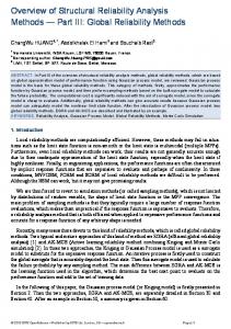
Based on the maximum likelihood estimation in (4), the values of each Copula function’s correlation parameter 𝜃 were calculated and are listed in Table 7. The 3D joint probability density function 𝑓(𝑌, 𝑍, 𝑤) and the performance function 𝑔(𝑌, 𝑍, 𝑤) in example 2 were substituted into (13) to calculate the integrand. The structure of the integrand neural network could also be constructed. The integrand neural network had three inputs and single output. After adjustment, the number of

hidden layer units is 𝑚 = 10. The transfer functions of hidden layer and output layer were 𝑓𝑠 = 𝑒𝑥 and Purelin function, respectively. Variables 𝑌, 𝑍, and 𝑤 were separately divided into 30 parts in the range of [𝜇𝑖 − 3𝜎𝑖 , 𝜇𝑖 + 3𝜎𝑖 ]. The three variables intersect each other to form the integrand network input sample point. The network output value 𝑦 of the corresponding sample point was calculated by the integrand function, and the training sample point set is shown in Table 8. We used the Levenberg-Marquardt training algorithm. When the training reached 100 steps, the error of the integrand network reached the convergence state. The error convergence curve is shown in Figure 5. The integrand network training sample set of each vertex in a hypercube was calculated and simulated with the original function network. The sample set is shown in Table 9. The results were substituted into (18) to obtain the result of reliability. Nataf-MCS was introduced in Section 3. The sampling was 1,000,000 times, and the reliability of example 2 was 0.9998. In this example, 𝛾 = 35.71. Table 10 shows the reliability values calculated by the two methods. In this example, three kinds of Archimedean Copula functions were selected to construct the joint probability density function of variables 𝑌, 𝑍, and 𝑤. The reliability of the proposed method was 0.85%, which was higher than that of Nataf-MCS. The ratio 𝛾 of calculation workload was 35.71, indicating that the proposed method has superior computational efficiency and can reduce the calculation time.

8

Mathematical Problems in Engineering Table 8: Training sample set of integrand network in example 2.

𝑌 626.40 626.40 ⋅⋅⋅ 626.40 ⋅⋅⋅ 1351.10 1351.10 ⋅⋅⋅ 1351.10

𝑌

𝑍

𝑤

108.84 136.25 ⋅⋅⋅ 903.70 ⋅⋅⋅ 108.84 136.25 ⋅⋅⋅ 903.70

1.17 3.7406𝑒 − 019 6.1769𝑒 − 019 ⋅⋅⋅ 1.1581𝑒 − 020 ⋅⋅⋅ 7.8195𝑒 − 021 1.2385𝑒 − 020 ⋅⋅⋅ 1.3654𝑒 − 022

⋅⋅⋅ ⋅⋅⋅ ⋅⋅⋅ ⋅⋅⋅ ⋅⋅⋅ ⋅⋅⋅ ⋅⋅⋅ ⋅⋅⋅ ⋅⋅⋅ ⋅⋅⋅

1.23 7.2479𝑒 − 019 1.1926𝑒 − 018 ⋅⋅⋅ 2.1592𝑒 − 020 ⋅⋅⋅ 1.4568𝑒 − 020 2.3063𝑒 − 020 ⋅⋅⋅ 2.5241𝑒 − 022

2.74 2.0566𝑒 − 017 3.3278𝑒 − 017 ⋅⋅⋅ 4.9973𝑒 − 019 ⋅⋅⋅ 3.3560𝑒 − 019 5.2996𝑒 − 019 ⋅⋅⋅ 5.5421𝑒 − 021

2.80 9.2777𝑒 − 019 1.4721𝑒 − 018 ⋅⋅⋅ 1.6704𝑒 − 020 ⋅⋅⋅ 1.1119𝑒 − 020 1.7472𝑒 − 020 ⋅⋅⋅ 1.6625𝑒 − 022

Table 9: Simulative sample set of original function network in example 2. 𝑌 𝑍 𝑤

626.40 108.84 1.17

1351.10 903.70 2.80

626.40 108.84 2.80

1351.10 108.84 2.80

626.40 903.70 1.17

1351.10 108.84 1.17

626.40 903.70 2.80

1351.10 903.70 1.17

Table 10: Example 2 reliability calculation results. Method

Nataf-MCS

Reliability Relative error (%)

Frank Copula

0.9998 0

0.9960 0.38

LI 1.28 1.27 1.45 1.20 1.26 ⋅⋅⋅ 2.11 2.05 1.57

𝑠𝑢 (kPa) 2.58 4.74 5.42 5.82 6.97 ⋅⋅⋅ 12.26 14.10 15.20

𝑠𝑢re (kPa) 0.22 0.16 0.39 0.59 0.65 ⋅⋅⋅ 1.53 1.53 1.84

𝜎𝑝󸀠 (kPa) 7.94 29.41 17.14 27.63 23.37 ⋅⋅⋅ 80.24 86.36 94.76

0.9913 0.85

0.9936 0.62

𝜌

Table 11: Test data for soil parameters. Number 1 2 3 4 5 ⋅⋅⋅ 343 344 345

Direct integral method based on dual neural network Gumbel Copula Clayton Copula

𝜎V󸀠 (kPa) 9.56 12.82 16.44 20.06 24.04 ⋅⋅⋅ 61.90 68.02 75.66

5.3. Example 3. The soil parameters of rock and soil include liquidity index (LI), undrained shear strength 𝑠𝑢 , remolded undrained shear strength 𝑠𝑢re , preconsolidation stress 𝜎𝑝󸀠 , and vertical effective stress 𝜎V󸀠 . The experimental data in literature [53] were used as an example to illustrate the calculation steps of the proposed method. The performance function of the soil parameters 𝑔(LI, 𝑠𝑢 , 𝑠𝑢re , 𝜎𝑝󸀠 , 𝜎V󸀠 ) = 𝜎𝑝󸀠 (𝑠𝑢re +LI𝜎𝑝󸀠 )−(𝜎V󸀠 −𝑠𝑢 )2 was considered, and the reliability of rock and soil was analyzed under normal use limit state. Test data for soil parameters are shown in Table 11. The mean 𝜇, standard deviation 𝜎, and edge distribution functions type of each variable were obtained by analyzing the experimental data as shown in Table 12. From the calculation, we obtained the correlation coefficient 𝜌𝑖𝑗 of any two variables to form the matrix 𝜌.

LI =

𝑠𝑢 𝑠𝑢re 𝜎𝑝󸀠 𝜎V󸀠

LI

𝑠𝑢re

𝑠𝑢re

𝜎𝑝󸀠

𝜎V󸀠

1 [ [ 0.05 [ [ −0.50 [ [ [ −0.06 [ [ −0.21

0.05

−0.50

−0.06

−0.21

1

0.17

0.84

0.17

1

0.30

0.84

0.30

1

0.57

0.42

0.73

] 0.57 ] (23) ]. 0.42 ] ] ] 0.73 ] ] 1 ]

Given the positive and negative correlations among variables LI, 𝑠𝑢 , 𝑠𝑢re , 𝜎𝑝󸀠 , and 𝜎V󸀠 , we need to select the appropriate Copula function from Elliptical Copula function to construct the joint probability density function 𝑓(LI, 𝑠𝑢 , 𝑠𝑢re , 𝜎𝑝󸀠 , 𝜎V󸀠 ). Using AIC and BIC criteria, Gaussian Copula was selected for example 2. Afterwards, (3) was used to obtain any two variables related parameters 𝜃𝑖𝑗 and to form matrix 𝜃. 𝜃

LI =

𝑠𝑢 𝑠𝑢re 𝜎𝑝󸀠 𝜎V󸀠

LI

𝑠𝑢re

𝑠𝑢re

𝜎𝑝󸀠

𝜎V󸀠

1 [ [ 0.07 [ [ −0.91 [ [ [ −0.08 [ [ −0.26

0.07

−0.91

−0.08

−0.26

1

0.25

0.88

0.25

1

0.41

0.88

0.41

1

0.64

0.53

0.78

] 0.67 ] (24) ]. 0.53 ] ] ] 0.78 ] ] 1 ]

Mathematical Problems in Engineering

9

Table 12: Statistical parameters and distribution types of variables in example 3. Items Mean 𝜇 Standard deviation 𝜎 Edge distributionfunction

LI

𝑠𝑢 (kPa)

𝑠𝑢re (kPa)

𝜎𝑝󸀠 (kPa)

𝜎V󸀠 (kPa)

1.25 0.61 Lognormal

31.01 29.48 Lognormal

2.51 3.81 Lognormal

105.82 103.21 Lognormal

66.63 53.48 Lognormal

415.45 201.85 4.1945𝑒 − 011 1.3897𝑒 − 011 ⋅⋅⋅ 2.5274𝑒 − 013 ⋅⋅⋅ 5.8267𝑒 − 014 1.7905𝑒 − 014 ⋅⋅⋅ 1.7823𝑒 − 016

415.45 227.07 2.7672𝑒 − 011 9.2053𝑒 − 012 ⋅⋅⋅ 1.7285𝑒 − 013 ⋅⋅⋅ 3.7218𝑒 − 014 1.1483𝑒 − 014 ⋅⋅⋅ 1.1802𝑒 − 016

Table 13: Training sample set of integrand network in example 3. LI 0.10 0.10 ⋅⋅⋅ 0.10 ⋅⋅⋅ 3.08 3.08 ⋅⋅⋅ 3.08

𝑠𝑢

𝑠𝑢re

0.10 0.10 ⋅⋅⋅ 0.10 ⋅⋅⋅ 119.45 119.45 ⋅⋅⋅ 119.45

0.10 1.64 ⋅⋅⋅ 13.94 ⋅⋅⋅ 0.10 1.64 13.94

𝜎𝑝󸀠 𝜎V󸀠

𝑦 0.10 0.10 1.0728𝑒 − 006 3.3559𝑒 − 007 ⋅⋅⋅ 3.8546𝑒 − 009 ⋅⋅⋅ 1.3303𝑒 − 010 3.8597𝑒 − 011 ⋅⋅⋅ 2.4266𝑒 − 013

0.10 25.32 5.3550𝑒 − 007 1.6819𝑒 − 007 ⋅⋅⋅ 1.9948𝑒 − 009 ⋅⋅⋅ 6.4296𝑒 − 011 1.8729𝑒 − 011 ⋅⋅⋅ 1.2159𝑒 − 013

The 5D joint probability density function of variables LI, 𝑠𝑢 , 𝑠𝑢re , 𝜎𝑝󸀠 , and 𝜎V󸀠 can be expressed as the following equation:

⋅⋅⋅ ⋅⋅⋅ ⋅⋅⋅ ⋅⋅⋅ ⋅⋅⋅ ⋅⋅⋅ ⋅⋅⋅ ⋅⋅⋅ ⋅⋅⋅ ⋅⋅⋅

Performance is 7.72093e − 012; goal is 0

10−10

= 𝑓 (LI) 𝑓 (𝑠𝑢 ) 𝑓 (𝑠𝑢re ) 𝑓 (𝜎𝑝󸀠 ) 𝑓 (𝜎V󸀠 )

(25)

⋅ 𝑐 (𝐹 (LI) , 𝐹 (𝑠𝑢 ) , 𝐹 (𝑠𝑢re ) , 𝐹 (𝜎𝑝󸀠 ) , 𝐹 (𝜎V󸀠 ) ; 𝜃) . The 5D joint probability density function 𝑓(LI, 𝑠𝑢 , 𝑠𝑢re , 𝜎𝑝󸀠 , 𝜎V󸀠 ) and the performance function 𝑔(LI, 𝑠𝑢 , 𝑠𝑢re , 𝜎𝑝󸀠 , 𝜎V󸀠 ) were substituted into (13) to calculate the integrand. The structure of the integrand neural network could also be constructed. The integrand neural network had five inputs and single output. After adjustment, the number of hidden layer units was 𝑚 = 5. The transfer functions of hidden layer and output layer were 𝑓𝑠 = 𝑒𝑥 and Purelin function, respectively. Variables LI, 𝑠𝑢 , 𝑠𝑢re , 𝜎𝑝󸀠 , and 𝜎V󸀠 are divided into 10 parts in the range of [𝜇𝑖 − 4𝜎𝑖 , 𝜇𝑖 + 5𝜎𝑖 ]. The five variables intersect each other to form the input sample points of the integrand network. The network output value 𝑦 of the corresponding sample points was calculated by the integrand function. Given that each variable follows the lognormal distribution, we get 𝜇𝑖 − 4𝜎𝑖 = 0.1 when the left interval of the variable 𝜇𝑖 − 4𝜎𝑖 ≤ 0. The training sample set is shown in Table 13. We used the Levenberg-Marquardt training algorithm. When the training reached 100 steps, the error of the integrand network reached the convergence state. The error convergence curve is shown in Figure 6. We used the same method for the previous example. The sample points of the original function network were obtained and are shown in Table 14. The simulation values

Training-blue

𝑓 (LI, 𝑠𝑢 , 𝑠𝑢re , 𝜎𝑝󸀠 , 𝜎V󸀠 )

10−11

10−12

0

Stop training

20

40 60 100 epochs

80

100

Figure 6: Training error curve of integrand network in example 3.

were substituted into (18) to obtain the reliability of the structure as shown in Table 15. The calculation workload of the two methods was substituted into (21), thus obtaining 𝛾 = 9.90. The reliability of 5D correlated variables is analyzed using example 3. The reliability of the proposed method was extremely close to that of Nataf-MCS, and the relative error was only 1.16%. From 𝛾 = 9.90, for the same problem, the workload of the two methods varied greatly. The neural network method has advantages in computational efficiency and reduces the calculation time for structural reliability analysis. This example shows that the proposed method can

10

Mathematical Problems in Engineering Table 14: Simulative sample set of original function network in example 3.

LI 𝑠𝑢 𝑠𝑢re 𝜎𝑝󸀠 𝜎V󸀠

0.10 0.10 0.10 0.10 0.10

3.08 119.45 13.94 415.45 227.07

0.10 119.45 13.94 415.45 227.07

⋅⋅⋅ ⋅⋅⋅ ⋅⋅⋅ ⋅⋅⋅ ⋅⋅⋅

3.08 0.10 0.10 0.10 0.10

0.10 0.10 13.94 0.10 227.07

3.08 119.45 0.10 415.45 0.10

Table 15: Example 3 reliability calculation results. Method Reliability Relative error (%)

Nataf-MCS 0.9594 0

efficiently solve the reliability problem of multidimensional correlated variables.

6. Conclusion Identifying the joint probability density function among variables is necessary to accurately calculate the structural reliability. This paper used the Copula function to construct the joint probability density function among correlated variables. According to Copula theory, the estimation of the edge probability density function among variables is independent of the selection of Copula function. The joint distribution function with arbitrary edge distribution and correlation structure could be constructed. This method was suitable for constructing joint probability density functions of 2D and multidimensional correlation problems. In addition, this paper proposed a Monte Carlo method based on Nataf inverse transformation. Nataf-MCS and the proposed method were used to solve the structural reliability among correlated variables. The proposed method could overcome the difficulty of solving multiple integral problems and achieve accurate calculation of reliability. However, we did not establish the relationship of the original function and every random variable because the training sample set originated from the integrand. We conveniently selected the sample set to improve the accuracy of calculating the reliability. Numerical examples showed that the proposed method is highly precise and efficient in calculating the reliability of multidimensional correlated variables. Copula function is often used to construct the static variable correlation model. In many applications, the correlation coefficient among variables has the characteristics of being dynamic and time-varying. Thus, a Copula model must be constructed to describe the effect of these factors on structural reliability. This issue must be further explored. In future work, the proposed method can also be extended for the reliability analysis of large and complex structural problems. In these cases, the workload of computing for dual neural network was negligible as compared with that of constructing network training samples. In addition, (21) can be simplified to 𝛾 ≈ 𝑁𝑚 /𝑁𝑛 . Hence, the proposed method shows efficiency and advantages in analyzing large and complex structural problems.

Direct integral method based on dual neural network Gaussian Copula 0.9483 1.16

Conflicts of Interest The authors declare that there are no conflicts of interest regarding the publication of this paper.

Acknowledgments This work was supported by the National Natural Science Foundation of China under Grant no. 11262014 and Graduate Student Scientific Research Innovation Project of Autonomous Region under Grant no. B20171012805.

References [1] K. Goda, “Statistical modeling of joint probability distribution using copula: Application to peak and permanent displacement seismic demands,” Structural Safety, vol. 32, no. 2, pp. 112–123, 2010. [2] B. J. Leira, “Probabilistic assessment of weld fatigue damage for a nonlinear combination of correlated stress components,” Probabilistic Engineering Mechanics, vol. 26, no. 3, pp. 492–500, 2011. [3] D. Li, Y. Chen, W. Lu, and C. Zhou, “Stochastic response surface method for reliability analysis of rock slopes involving correlated non-normal variables,” Computers & Geosciences, vol. 38, no. 1, pp. 58–68, 2011. [4] D.-Q. Li, X.-S. Tang, K.-K. Phoon, Y.-F. Chen, and C.-B. Zhou, “Bivariate simulation using copula and its application to probabilistic pile settlement analysis,” International Journal for Numerical and Analytical Methods in Geomechanics, vol. 37, no. 6, pp. 597–617, 2013. [5] H. F. Burcharth, J. D. Sorensen, and E. Christian, “On the evaluation of failure probability of monolithic vertical wall breakwaters,” Proceedings of Wave Barriers in Deep Waters, pp. 458–468, 1994. [6] A. Der Kiureghian, H.-Z. Lin, and S.-J. Hwang, “Second-order reliability approximations,” Journal of Engineering Mechanics, vol. 113, no. 8, pp. 1208–1225, 1987. [7] S. Yue, “The bivariate lognormal distribution for describing joint statistical properties of a multivariate storm event,” Environmetrics, vol. 13, no. 8, pp. 811–819, 2002. [8] A. C. Rencher, Methods of Multivariate Analysis, John Wiley & Sons, Inc., New York, NY, USA, 1995. [9] R. B. Nelsen, An Introduction to Copulas, Springer, New York, NY, USA, 2nd edition, 2006.

Mathematical Problems in Engineering [10] M. Sklar, “Fonctions de repartition an dimensions et leurs marges,” Publications de l’Institut de Statistique de l’Universit´e de Paris, vol. 8, pp. 229–231, 1959. [11] X. Zeng, J. Ren, Z. Wang, S. Marshall, and T. Durrani, “Copulas for statistical signal processing (Part I): Extensions and generalization,” Signal Processing, vol. 94, no. 1, pp. 691–702, 2014. [12] Y. Li, B. Shi, and J. Zhang, “The copula joint function and its application in probabilistic seismic hazard analysis,” Earthquake Science, vol. 30, no. 3, pp. 292–301, 2008. [13] X.-S. Tang, D.-Q. Li, C.-B. Zhou, and K.-K. Phoon, “Probabilistic analysis of load-displacement hyperbolic curves of single pile using Copula,” Rock and Soil Mechanics, vol. 33, no. 1, pp. 171– 178, 2012. [14] D. Huang, C. Yang, B. Zeng, and G. Fu, “A copula-based method for estimating shear strength parameters of rock mass,” Mathematical Problems in Engineering, vol. 2014, Article ID 693062, 11 pages, 2014. [15] Z. Liu, X. Ma, J. Yang, and Y. Zhao, “Reliability modeling for systems with multiple degradation processes using inverse Gaussian process and copulas,” Mathematical Problems in Engineering, vol. 2014, Article ID 829597, 2014. [16] Y. Liu and X. Fan, “Time-independent reliability analysis of bridge system based on mixed copula models,” Mathematical Problems in Engineering, vol. 2016, Article ID 2720614, 13 pages, 2016. [17] X. Xu, J. Li, J. Gong, H. Deng, and L. Wan, “Copula-Based Slope Reliability Analysis Using the Failure Domain Defined by the gLine,” Mathematical Problems in Engineering, vol. 2016, Article ID 6141838, 11 pages, 2016. [18] I. Lee, K. K. Choi, and L. Zhao, “Sampling-based RBDO using the stochastic sensitivity analysis and dynamic kriging method,” Structural and Multidisciplinary Optimization, vol. 44, no. 3, pp. 299–317, 2011. [19] I. Lee, K. K. Choi, Y. Noh, L. Zhao, and D. Gorsich, “Samplingbased stochastic sensitivity analysis using score functions for RBDO problems with correlated random variables,” Journal of Mechanical Design, vol. 133, no. 2, Article ID 021003, 2011. [20] Y. Noh, K. K. Choi, and L. Du, “Reliability-based design optimization of problems with correlated input variables using a Gaussian Copula,” Structural and Multidisciplinary Optimization, vol. 38, no. 1, pp. 1–16, 2009. [21] Y. Noh, K. K. Choi, and I. Lee, “Identification of marginal and joint CDFs using Bayesian method for RBDO,” Structural and Multidisciplinary Optimization, vol. 40, no. 1-6, pp. 35–51, 2010. [22] Y. Noh, K. K. Choi, I. Lee, D. Gorsich, and D. Lamb, “Reliabilitybased design optimization with confidence level for nonGaussian distributions using bootstrap method,” Journal of Mechanical Design, vol. 133, no. 9, Article ID 091001, 2011. [23] Y. Noh, Input Model Uncertainty and Reliability-Based Design Optimization with Associated Confidence Level, The University of Iowa, Iowa, USA, 2009. [24] H. Cho, K. K. Choi, and D. Lamb, “Sensitivity developments for RBDO with dependent input variable and varying input standard deviation,” Journal of Mechanical Design, vol. 139, no. 7, 9 pages, 2017. [25] Y. Noh, K. K. Choi, and I. Lee, “Reduction of ordering effect in reliability-based design optimization using dimension reduction method,” AIAA Journal, vol. 47, no. 4, pp. 994–1004, 2009. [26] Y. Noh, K. K. Choi, I. Lee, D. Gorsich, and D. Lamb, “Reliabilitybased design optimization with confidence level under input

11

[27]

[28]

[29]

[30]

[31] [32]

[33]

[34]

[35]

[36]

[37]

[38]

[39]

[40]

[41]

[42]

model uncertainty due to limited test data,” Structural and Multidisciplinary Optimization, vol. 43, no. 4, pp. 443–458, 2011. Y. Noh, K. K. Choi, and I. Lee, “Comparison study between MCMC-based and weight-based Bayesian methods for identification of joint distribution,” Structural and Multidisciplinary Optimization, vol. 42, no. 6, pp. 823–833, 2010. H. Cho, K. K. Choi, I. Lee, and D. Lamb, “Design Sensitivity Method for Sampling-Based RBDO with Varying Standard Deviation,” Journal of Mechanical Design, vol. 138, no. 1, Article ID 011405, 2016. Y.-G. Zhao and T. Ono, “A general procedure for first/secondorder reliability method (FORM/SORM),” Structural Safety, vol. 21, no. 2, pp. 95–112, 1999. Y.-G. Zhao and T. Ono, “Third-moment standardization for structural reliability analysis,” Journal of Structural Engineering, vol. 126, no. 6, pp. 724–731, 2000. Y.-G. Zhao and T. Ono, “Moment methods for structural reliability,” Structural Safety, vol. 23, no. 1, pp. 47–75, 2001. Q. Gong, J. Zhang, C. Tan, and C. Wang, “Neural networks combined with importance sampling techniques for reliability evaluation of explosive initiating device,” Chinese Journal of Aeronautics, vol. 25, no. 2, pp. 208–215, 2012. V. Papadopoulos, D. G. Giovanis, N. D. Lagaros, and M. Papadrakakis, “Accelerated subset simulation with neural networks for reliability analysis,” Computer Methods Applied Mechanics and Engineering, vol. 223/224, pp. 70–80, 2012. R. Douc, F. Maire, and J. Olsson, “On the use of Markov chain MONte Carlo methods for the sampling of mixture models: a statistical perspective,” Statistics and Computing, vol. 25, no. 1, pp. 95–110, 2015. A. Genz and A. Malik, “Remarks on algorithm 006: An adaptive algorithm for numerical integration over an N-dimensional rectangular region,” Journal of Computational and Applied Mathematics, vol. 6, no. 4, pp. 295–299, 1980. M. Papadrakakis, V. Papadopoulos, and N. D. Lagaros, “Structural reliability analyis of elastic-plastic structures using neural networks and Monte Carlo simulation,” Computer Methods Applied Mechanics and Engineering, vol. 136, no. 1-2, pp. 145– 163, 1996. P. A. M. Lopes, H. M. Gomes, and A. M. Awruch, “Reliability analysis of laminated composite structures using finite elements and neural networks,” Composite Structures, vol. 92, no. 7, pp. 1603–1613, 2010. Y.-L. Zuo, H.-H. Zhu, and X.-J. Li, “An ANN-based four order moments method for geotechnical engineering reliability analysis,” Rock and Soil Mechanics, vol. 34, no. 2, pp. 513–518, 2013. J. Cheng and Q. S. Li, “Reliability analysis of structures using artificial neural network based genetic algorithms,” Computer Methods Applied Mechanics and Engineering, vol. 197, no. 45-48, pp. 3742–3750, 2008. W. Meng, Z. Yang, X. Qi, and J. Cai, “Reliability analysisbased numerical calculation of metal structure of bridge crane,” Mathematical Problems in Engineering, vol. 2013, Article ID 260976, 5 pages, 2013. A. H. Elhewy, E. Mesbahi, and Y. Pu, “Reliability analysis of structures using neural network method,” Probabilistic Engineering Mechanics, vol. 21, no. 1, pp. 44–53, 2006. H. B. Li, Y. He, and X. B. Nie, “Structural reliability calculation method based on the dual neural network and direct integration method,” Neural Computing and Applications, pp. 1–9, 2016.

12 [43] H. Dai and Z. Cao, “A Wavelet Support Vector Machine-Based Neural Network Metamodel for Structural Reliability Assessment,” Computer-Aided Civil and Infrastructure Engineering, vol. 32, no. 4, pp. 344–357, 2017. [44] U. Cherubini, E. Luciano, and W. Vecchiato, “Copula Methods in Finance,” Copula Methods in Finance, pp. 1–293, 2013. [45] H. Akaike, “A New Look at the Statistical Model Identification,” IEEE Transactions on Automatic Control, vol. 19, no. 6, pp. 716– 723, 1974. [46] G. Schwarz, “Estimating the dimension of a model,” The Annals of Statistics, vol. 6, no. 2, pp. 461–464, 1978. [47] Y. Hao, X. Rong, L. Ma, P. Fan, and H. Lu, “Uncertainty analysis on risk assessment of water inrush in karst tunnels,” Mathematical Problems in Engineering, vol. 2016, Article ID 2947628, 2016. [48] S. Mishra, O. A. Vanli, B. P. Alduse, and S. Jung, “Hurricane loss estimation in wood-frame buildings using Bayesian model updating: Assessing uncertainty in fragility and reliability analyses,” Engineering Structures, vol. 135, pp. 81–94, 2017. [49] A. Ang, -S. Tang W, and -S. Tang, Probability Concepts in Engineering Planning and Design, John Wiley and Sons, New York, NY, USA, 1984. [50] A. Nataf, “Determination des distributions de probabilites dont les marges sont donnees,” Comptes Rendus De L’academie Des Sciences, vol. 255, pp. 42-43, 1962. [51] A. Der Kiureghian and P.-L. Liu, “Structural reliability under incomplete probability information,” Journal of Engineering Mechanics, vol. 112, no. 1, pp. 85–104, 1986. [52] C. Jiang, W. Zhang, B. Wang, and X. Han, “Structural reliability analysis using a copula-function-based evidence theory model,” Computers & Structures, vol. 143, pp. 19–31, 2014. [53] J. Ching and K. Phoon, “Corrigendum: Modeling parameters of structured clays as a multivariate normal distribution,” Canadian Geotechnical Journal, vol. 49, no. 12, pp. 1447–1450, 2012.

Mathematical Problems in Engineering

Advances in

Operations Research Hindawi Publishing Corporation http://www.hindawi.com

Volume 2014

Advances in

Decision Sciences Hindawi Publishing Corporation http://www.hindawi.com

Volume 2014

Journal of

Applied Mathematics

Algebra

Hindawi Publishing Corporation http://www.hindawi.com

Hindawi Publishing Corporation http://www.hindawi.com

Volume 2014

Journal of

Probability and Statistics Volume 2014

The Scientific World Journal Hindawi Publishing Corporation http://www.hindawi.com

Hindawi Publishing Corporation http://www.hindawi.com

Volume 2014

International Journal of

Differential Equations Hindawi Publishing Corporation http://www.hindawi.com

Volume 2014

Volume 2014

Submit your manuscripts at https://www.hindawi.com International Journal of

Advances in

Combinatorics Hindawi Publishing Corporation http://www.hindawi.com

Mathematical Physics Hindawi Publishing Corporation http://www.hindawi.com

Volume 2014

Journal of

Complex Analysis Hindawi Publishing Corporation http://www.hindawi.com

Volume 2014

International Journal of Mathematics and Mathematical Sciences

Mathematical Problems in Engineering

Journal of

Mathematics Hindawi Publishing Corporation http://www.hindawi.com

Volume 2014

Hindawi Publishing Corporation http://www.hindawi.com

Volume 2014

Volume 2014

Hindawi Publishing Corporation http://www.hindawi.com

Volume 2014

#HRBQDSDĮ,@SGDL@SHBR

Journal of

Volume 201

Hindawi Publishing Corporation http://www.hindawi.com

Discrete Dynamics in Nature and Society

Journal of

Function Spaces Hindawi Publishing Corporation http://www.hindawi.com

Abstract and Applied Analysis

Volume 2014

Hindawi Publishing Corporation http://www.hindawi.com

Volume 2014

Hindawi Publishing Corporation http://www.hindawi.com

Volume 2014

International Journal of

Journal of

Stochastic Analysis

Optimization

Hindawi Publishing Corporation http://www.hindawi.com

Hindawi Publishing Corporation http://www.hindawi.com

Volume 2014

Volume 2014