The Microstructure of Spoken Word Recognition by James ... - CiteSeerX

The Microstructure of Spoken Word Recognition by James Stephen Magnuson

Submitted in Partial Fulfillment of the Requirements for the Degree Doctor of Philosophy Supervised by Professor Michael K. Tanenhaus and Professor Richard N. Aslin Department of Brain and Cognitive Sciences The College Arts and Sciences University of Rochester Rochester, New York 2001

ii

Dedication To Inge-Marie Eigsti, for your love and support, advice on research and everything else, picking me up when I’m down, and making grad school a whole lot of fun.

iii

Curriculum Vitae The author was born December 19th, 1968, in St. Paul, Minnesota, and grew up on a farm 50 miles north of the Twin Cities. He received the A.B. degree in linguistics with honors from the University of Chicago in 1993. After two years as an intern researcher at Advanced Telecommunications Research Human Information Processing Laboratories in Kyoto, Japan, he began the doctoral program in Brain and Cognitive Sciences at the University of Rochester. The author worked in the labs of Professor Michael Tanenhaus and Professor Mary Hayhoe in his first three years at Rochester. In both labs, he used eye tracking as an incidental measure of processing (language processing in the former, visuospatial working memory in the latter). As his dissertation work focused on spoken word recognition, Michael Tanenhaus continued as his primary advisor, and Professor Richard Aslin became his co-advisor. The author was supported by a National Science Foundation Graduate Research Fellowship (1995-1998), a University of Rochester Sproull Fellowship (1998-2000), and a Grant-in-Aid-of-Research from the National Academy of Sciences through Sigma Xi. He received the M.A. degree in Brain and Cognitive Sciences in 2000.

iv

Acknowledgements My parents, through life-long example, have taught me the importance of family and hard work. I am grateful for the sacrifices they made, and the love and support they gave me, which made it possible for me to be writing this today. Several middle- and high-school teachers encouraged and inspired me in an environment where intellectual pursuits were not always valued: Mary Ruprecht, David Jaeger, Tim Johnson, Kay Pekel, and Howard Lewis. Terry and Susan Wolkerstorfer played instrumental roles in my skin-of-the-teeth acceptance to the University of Chicago, and have been great friends since. During a year off, I had some adventures and seriously considered not returning to college. I thank Henry Bromelkamp for ‘firing’ me and encouraging me to finish. At Chicago, Nancy Stein’s introductory lecture for “Cognition and Learning” first got me hooked on cognitive science. My interest grew into passion under Howard Nusbaum’s tutelage. His enthusiasm and curiosity inspired my own, and I will always look up to Howard’s example. I learned working for Gerd Gigerenzer that science ought to be a lot of fun. At ATR in Japan, Reiko Akahane-Yamada was my teacher and role model; her example confirmed my decision to pursue a Ph.D. I also learned a lot from Yoh’ichi Tohkura, Hideki Kawahara, Eric Vatikiosis-Bateson, Kevin Munhall, Winifred Strange, and John Pruitt. I am extremely fortunate to have been able to pursue my Ph.D. at Rochester. Mike Tanenhaus always provided just the right mixture of guidance, support and freedom. Throughout the challenges of graduate school, Mike’s constant encouragement, wit, and the occasional gourmet Asian feast helped keep me going. Mary Hayhoe taught me a lot about how to tackle very difficult aspects of perception and cognition experimentally. Her approach to perception and action in natural contexts has had a huge impact on my interests and thinking. Dick Aslin is always ready with sage advice on any topic. His Socratic knack for asking the question that cuts to the essence of a problem has led me out of many intellectual and experimental

v

jams. I thank Joyce McDonnough for being part of my proposal committee, and James Allen for being a member of my dissertation committee. An especially important part of my experience at Rochester was collaborating with post-docs and other students. Paul Allopenna taught me a lot about speech, neural networks, risotto, and the guitar, and helped me through some difficult periods. Delphine Dahan let me join her on three elegant projects. Paul and Delphine were wonderful mentors, and the projects I did with them led to the work reported here. Dave Bensinger showed me how to keep things in perspective. I’m still learning from my current collaborators, Craig Chambers, Jozsef Fiser, and Bob McMurray. My graduate school experience was shaped largely by a number of fellow students, post-docs and friends, but in particular, Craig Chambers, Marie Coppola, Jozsef Fiser, Josh Fitzgerald, Carla Hudson, Ruskin Hunt, Cornell Juliano, Sheryl Knowlton, Toby Mintz, Seth Pollak, Jenny Saffran, Annie Senghas, Steve Shimozaki, Michael Spivey, Julie Sedivy, and Whitney Tabor. I was completely dependent on the expertise, encouragement and friendly faces) of administrators and technical staff in BCS and the Center for Visual Sciences, especially Bette McCormick, Kathy Corser, Jennifer Gillis, Teresa Williams, Barb Arnold, Judy Olevnik, and Bill Vaughn. Several research assistants in the Tanenhaus lab provided invaluable help running subjects and coding data. Dana Subik was especially helpful and fun to work with, and provided the organization, good humor, and patience that allowed me to finish on time. It’s only a slight exaggeration to say that I owe my sanity and new job to hockey. I thank Greg Carlson, George Ferguson, and the Rochester Rockets for getting me back into hockey. Moshi-Moshi Neko and Henri Matisse were soothing influences, and made sure I exercised everyday. I’m grateful for support from a National Science Foundation Graduate Research Fellowship, a University of Rochester Sproull Fellowship, a Grant-in-Aidof-Research from the National Academy of Sciences through Sigma Xi, and from grants awarded to my advisors, M. Tanenhaus, M. Hayhoe, and R. Aslin.

vi

Abstract This dissertation explores the fine-grained time course of spoken word recognition: which lexical representations are activated over time as a word is heard. First, I examine how bottom-up acoustic information is evaluated with respect to lexical representations. I measure the time course of lexical activation and competition during the on-line processing of spoken words, provide the first time course measures of neighborhood effects in spoken word recognition, and demonstrate that similarity metrics must take into account the temporal nature of speech, since, e.g., similarity at word onset results in stronger and faster activation than overlap at offset. I develop a paradigm combining eye tracking as participants follow spoken instructions to perform visually-guided tasks with a set of displayed objects (providing a fine-grained time course measure) with artificial lexicons (providing precise control over lexical characteristics), as well as replications and extensions with real words. Control experiments demonstrate that effects in this paradigm are not driven solely by the visual display, and, in the context of an experiment, artificial lexicons are functionally encapsulated from a participant’s native lexicon. The second part examines how top-down information is incorporated into online processing. Participants learned a lexicon of nouns (referring to novel shapes) and adjectives (novel textures). Items had phonological competitors within their syntactic class, and in the other. Items competed with similar, within-class items. In contrast to real-word studies, competition was not observed between items from different form classes in contexts where the visual display provided strong syntactic expectations (a context requiring an adjective vs. one where an adjective would be infelicitous). I argue that (1) this pattern is due to the highly constraining context, in contrast to the ungrounded materials used previously with real words, and (2) the impact of top-down constraints depends on their predictive power. The work reported here establishes a methodology that provides the finegrained time course measure and precise stimulus control required to uncover the

vii

microstructure of spoken word recognition. The results provide constraints on theories of word recognition, as well as language processing more generally, since lexical representations are implicated in aspects of syntactic, semantic and discourse processing.

viii

Table of Contents Dedication ..................................................................................................................... ii Curriculum Vitae ......................................................................................................... iii Acknowledgements...................................................................................................... iv List of Tables ................................................................................................................ x List of Figures .............................................................................................................. xi Foreword ..................................................................................................................... xii

Chapter 1: Introduction and overview ................................................................ 1 The macrostructure of spoken word recognition .......................................................... 3 The microstructure of spoken word recognition........................................................... 6

Chapter 2: The “visual world” paradigm ......................................................... 10 The apparatus and rationale ........................................................................................ 10 Vision and eye movements in natural, ongoing tasks................................................. 13 Language-as-product vs. language-as-action.............................................................. 17 The microstructure of lexical access: Cohorts and rhymes ........................................ 18

Chapter 3: Studying time course with an artificial lexicon ......................... 26 Experiment 1............................................................................................................... 29 Method ................................................................................................................ 29 Results................................................................................................................. 34 Discussion ........................................................................................................... 39 Experiment 2............................................................................................................... 39 Method ................................................................................................................ 40 Results................................................................................................................. 40 Discussion ........................................................................................................... 43 Discussion of Experiments 1 and 2............................................................................. 43

Chapter 4: Replication with English stimuli ................................................... 46 Experiment 3............................................................................................................... 47 Methods............................................................................................................... 47 Predictions........................................................................................................... 49 Results................................................................................................................. 49 Discussion ........................................................................................................... 55 Chapter 5: Do newly learned and native lexicons interact? ........................ 57 Experiment 4............................................................................................................... 58 Methods............................................................................................................... 58

ix

Predictions........................................................................................................... 62 First block ................................................................................................................... 62 Last block.................................................................................................................... 62 Results................................................................................................................. 62 Discussion ........................................................................................................... 66 Conclusion .......................................................................................................... 69 Chapter 6: Top-down constraints on word recognition ................................ 70 Experiment 5............................................................................................................... 73 Methods............................................................................................................... 73 Predictions........................................................................................................... 78 Results................................................................................................................. 79 Discussion ........................................................................................................... 82 Chapter 7: Summary and Conclusions ............................................................. 84 References................................................................................................................... 86 Appendix: Materials used in Experiment 3 ................................................................ 95

x

List of Tables Table 3.1: Accuracy in training and testing in Experiment 1. .................................... 36 Table 3.2: Accuracy in training and testing in Experiment 2. .................................... 41 Table 4.1: Frequencies and neighborhood and cohort densities in Experiment 3. ..... 48 Table 5.1: Linguistic stimuli from Experiment 4........................................................ 59 Table 5.2: Progression of training and testing accuracy in Experiment 4. ................. 62 Table 6.1: Artificial lexicon used in Experiment 5..................................................... 74 Table 6.2: Progression of accuracy in Experiment 5. ................................................. 79

xi

List of Figures Figure 1.1: A schematic of the language processing system. ....................................... 5 Figure 2.1: Eye tracking methodology........................................................................ 12 Figure 2.2: The block-copying task. ........................................................................... 13 Figure 2.3: Activations over time in TRACE. ............................................................ 20 Figure 2.4: Fixation proportions from Experiment 1 in Allopenna et al. (1998)........ 21 Figure 2.5: TRACE activations converted to response probabilities.......................... 24 Figure 3.1: Examples of 2AFC (top) and 4AFC displays from Experiments 1 and 2.31 Figure 3.2: Day 1 test (top) and Day 2 test (bottom) from Experiment 1................... 33 Figure 3.3: Cohort effects on Day 2 in Experiment 1................................................. 35 Figure 3.4: Rhyme effects on Day 2 in Experiment 1. ............................................... 37 Figure 3.5: Combined cohort and rhyme conditions in Experiment 2........................ 42 Figure 3.6: Effects of absent neighbors in Experiment 2............................................ 44 Figure 4.1: Main effects in Experiment 3. .................................................................. 51 Figure 4.2: Interactions of frequency with neighborhood and cohort density............ 52 Figure 4.3: Neighborhood density at levels of frequency and cohort density. ........... 53 Figure 4.4: Cohort density at levels of frequency and neighborhood density. ........... 54 Figure 5.1: Examples of visual stimuli from Experiment 4........................................ 60 Figure 5.2: Frequency effects on Day 1 (left) and Day 2 (right) of Experiment 4. .... 64 Figure 5.3: Density effects on Day 1 (left) and Day 2 (right) of Experiment 4.......... 65 Figure 6.1: The 9 shapes and 9 textures used in Experiment 5................................... 74 Figure 6.2: Critical noun conditions in Experiment 5................................................. 80 Figure 6.3: Critical adjective conditions in Experiment 5. ......................................... 81

xii

Foreword All of the experiments reported here were carried out with Michael Tanenhaus and Richard Aslin. Delphine Dahan collaborated on Experiments 1 and 2.

1

Chapter 1: Introduction and overview Linguistic communication is perhaps the most astonishing aspect of human cognition. In an instant, we transmit complex and abstract messages from one brain to another. We convert a conceptual representation to a linguistic one, and concurrently convert the linguistic representation to a series of motor commands that drive our articulators. In the case of spoken language, the acoustic energy of these articulations is transformed from mechanical responses of hair cells in our listener’s ears to a cortical representation of acoustic events which in turn must be interpreted as linguistic forms, which then are translated into conceptual information, which (usually) is quite similar to the intended message. Psycholinguistics is concerned largely with the mappings between conceptual representations and linguistic forms, and between linguistic forms and acoustics. Words provide the central interface in both of these mappings. Conceptual information must be mapped onto series of word forms, and in the other direction, words are where acoustics first map onto meaning. Some recent theories of sentence processing suggest that word recognition is not merely an intermediary stage that provides the input to syntactic and semantic processing. Instead, various results suggest that much of syntactic and semantic knowledge is associated with the representations of individual words in the mental lexicon (e.g., MacDonald, Pearlmutter, and Seidenberg, 1994; Trueswell and Tanenhaus, 1994). In the domain of spoken language, lexical knowledge is implicated in aspects of speech recognition that were often previously viewed as pre-lexical (Andruski, Blumstein, and Burton, 1994; Marslen-Wilson and Warren, 1994). Thus, how lexical representations are accessed during spoken word recognition has important implications for language processing more generally. However, a complicating factor in the study of spoken words is the temporal nature of speech. Words are comprised of sequences of transient acoustic events. Understanding how acoustics are mapped onto lexical representations requires that

2

we analyze the time course of lexical activation; knowing which words are activated as a word is heard provides strong constraints on theories of word recognition. The experiments we report here address two aspects of word recognition where time course measures are crucial. The first set of experiments addresses how the bottom-up acoustic signal is mapped onto linguistic representations. Spoken words, unlike visual words, are not unitary objects that can persist in time. Spoken words are comprised of series of overlapping, transient acoustic events. The input must be processed in an incremental fashion. As a word unfolds in time, the set of candidate representations potentially matching the bottom-up acoustic signal will change (cf., e.g., Marslen-Wilson, 1987). Different theories of spoken word recognition make different predictions about the nature of the activated competitor set over time (e.g., Marslen-Wilson, 1987, vs. Luce and Pisoni, 1998); thus, we need to be able to measure the activations of different sorts of competitors as words are processed in order to distinguish between models. In addition, top-down information sources are integrated with bottom-up acoustic information during word recognition, as we will review shortly. Knowing when and how top-down information sources are integrated will provide strong constraints on the development of theories and models of language processing. Specifically, we will examine whether a combination of highly predictive syntactic and pragmatic information can constrain the lexical items considered as possible matches to an input, or whether spoken word recognition initially operates primarily on bottom-up information. While this question has been addressed before, the pragmatic aspect – a visual display providing discourse constraints – is novel. A further contribution of this dissertation is the development of a methodology that addresses the psycholinguist’s perennial dilemma. Words in natural languages do not fall, in sufficient numbers, into neat categories of combinations of characteristics of interest, such as frequency and number of neighbors (similar sounding words), making it difficult to conduct precisely controlled factorial experiments. By creating artificial lexicons, we can instantiate just such categories. In

3

the rest of this chapter, we will set the stage for the experiments reported in this dissertation by reviewing the macrostructure and microstructure of spoken word recognition. The macrostructure of spoken word recognition A set of important empirical results must be accounted for by any theory of spoken word recognition. These principles form what Marslen-Wilson (1993) referred to as the macrostructure of spoken word recognition: the general constraints on possible architectures of the language processing system from the perspective of spoken word recognition. At the most general level, current models employ an activation metaphor, in which a spoken input activates items in the lexicon as a function of their similarity to the input and item-specific information (such as the frequency of occurrence). Activated items compete for recognition, also as a function of similarity and item-specific characteristics. We will not extensively review the results supporting each of these constraints. Instead, consider results from Luce and Pisoni (1998), which illustrate all of the constraints. According to their Neighborhood Activation Model (NAM), lexical items are predicted to be activated by a given input according to an explicit similarity metric.1 The probability of identifying each item is given by its similarity to the input multiplied by its log frequency of occurrence divided by the sum of all items’ frequency-weighted similarities. Similar items are called neighbors, and a word’s neighborhood is defined as the sum of the log-frequency weighted similarities of all words (the similarities between most words will effectively be zero). The rule that generates single-point predictions of the difficulty of identifying words is called the “frequency-weighted neighborhood probability rule”.

1

Typically, the metric is similar to that proposed by Coltheart, Davelaar, Jonasson and Besner (1977) for visual word recognition (items are predicted to be activated by an input if they differ by no more than one phoneme substitution, addition or deletion), or is based on confusion matrices collected for diphones presented in noise.

4

Luce and Pisoni report that item frequency alone accounts for about 5% of the variance in a variety of measures, including lexical decision response times, and frequency-weighted neighborhood accounts for significantly more (16-21%). So first we see that item characteristics (e.g., frequency) largely determine how quickly words can be recognized. Second, the fact that neighborhood is a good predictor of recognition time shows that (a) multiple items are being activated, (b) those items compete for recognition (since recognition time is inversely proportional to the number of competitors, weighted by frequency, suggesting that as an input is processed, all words in the neighborhood are activated and competing), and (c) items compete both as a function of similarity and frequency (frequency weighted neighborhood accounts for 10 to 15% more variance than simple neighborhood). At the macro level, there are four more central phenomena that models of spoken word recognition should account for. First, there is form priming. Goldinger, Luce and Pisoni (1989) reported that phonetically related words should cause inhibitory priming. Given first one stimulus (e.g., “veer”) and then a related one (e.g., “bull”, where each phoneme is highly confusable with its counterpart in the first stimulus), recognition should be slowed compared to a baseline condition where the second stimulus follows an unrelated item. The reason inhibition is predicted is that the first stimulus is predicted to activate both stimuli initially, but the second stimulus will be inhibited by the first (assuming an architecture such as TRACE’s, or Luce, Goldinger, Auer and Vitevitch’s [2000] implementation of the NAM, dubbed “PARSYN”). If the second stimulus is presented before its corresponding word form unit returns to its resting level of activation, its recognition will be slowed. These effects have generated considerable controversy (see Monsell and Hirsh, 1998, for a critical review). However, Luce et al. (2000) review a series of past studies and present some new ones that provide compelling evidence for inhibitory form (or “phonetic”) priming. Second, there is associative or semantic priming, by which a word like “chair” can prime a phonetically unrelated word like “table” due to their semantic

5

relatedness. Third, there is cross-modal priming (e.g., Tanenhaus, Leiman and Seidenberg, 1979; Zwitserlood, 1989), in which words presented auditorily affect the perception of phonologically or semantically related words presented visually. Finally, there are context effects. These include syntactic and semantic effects, where a listener is biased towards one interpretation of an ambiguous sequence by its sentence (or larger discourse) context (see Tanenhaus and Lucas, 1987, for a review).

Discourse/ Discourse/ Pragmatics Pragmatics Syntax/ Syntax/ Parsing Parsing

Semantics Semantics Lexicon Lexicon

Word forms Spoken word recognition

Visual Visualword word recognition recognition

Phonemes Acousticphonetic features

Auditory Auditory processing processing ofofacoustic acoustic input input

Figure 1.1: A schematic of the language processing system.

Figure 1.1 shows schematically the components of the language processing system implicated in the spoken word recognition literature. Components represented by ‘clouds’ are not implemented in any current model of spoken word recognition (although models for these exist in other areas of language research). These are

6

depicted as separate components merely for descriptive purposes; we will not discuss the degree to which any of them can be considered independent modules here. The microstructure of spoken word recognition Marslen-Wilson (1993) contrasted two levels at which one could formulate a processing theory. First, there are questions about the global properties of the processing system. A theory based on such a “macrostructural” perspective focuses on fairly coarse (but nonetheless important) questions such as what constraints there are on the general class of possible models. For spoken word recognition, these include the factors we discussed in the previous section. Armed with knowledge about the general properties required of a model, one can proceed to the more precise, “microstructural” level, and address fine-grained issues such as interactions among processing predictions for specific stimuli, modeling and measuring the time course of processing, and questions of how representations are learned. There is no black-and-white distinction between macro- and microstructural “levels.” Rather, there is a continuum. For example, Luce’s NAM (Luce, 1986; Luce and Pisoni, 1998) identifies some global, macrostructural constraints, but at the same time, makes such fine-grained predictions as response times for individual items. Why, then, have we taken, “the microstructure of spoken word recognition,” as our title? Two reasons are especially important. First, as Marslen-Wilson (1993) implied, the time has come for research on spoken word recognition to address the microstructure end of the continuum. There is consensus on the general properties of the system, but the field lacks a realistic theory or model with sufficient depth to account for microstructure, while maintaining sufficient breadth to obey the known macrostructural constraints (in other words, there are microtheories or micromodels of specific phenomena, but no sufficiently general theories or models; cf. Nusbaum and Henly, 1992). The best-known, bestworked out, explicit, implemented model of spoken word recognition remains the TRACE model (McClelland and Elman, 1986). While it suffers from various

7

computational problems (e.g., Elman, 1989; Norris, 1994), and cannot account for a number of basic speech perception phenomena, such as rate or talker normalization (e.g., Elman, 1989), it is the best game in town sixteen years later. One central factor in the slow rate of progress in developing theories of spoken word recognition has to do with a lag between the development of models of microstructure (such as TRACE and Cohort [e.g., Marslen-Wilson, 1987]) and sufficiently sensitive, direct and continuous measures to distinguish between them. As we will discuss in Chapter 2, the head-mounted eye tracking technique applied to language processing by Tanenhaus and colleagues (e.g., Tanenhaus et al., 1995) represents a large advance in our ability to measure the microstructure of language processing. The second reason to focus on microstructure has to do with what we argue to be an essential component of the microstructure approach: the use of precise mathematical models, or, in the case of simulating models (such as non-deterministic or incompletely understood neural networks), implemented models. Without precise, implemented models, there are limits to our ability to address even global properties of processing systems. Consider an example from visual perception. “Pop-out” phenomena in visual search are well known (see Wolfe, 1996, for a recent comprehensive review). Early explanations (which are still largely accepted) appealed to pre-attentive vs. attentive processes and resulting parallel or serial processing (e.g., Treisman and Gelade, 1980). Such verbal models appeared to be quite powerful. Many researchers replicated the diagnostic pattern. For searches based on a single feature, response time does not increase as the number of distractors does, suggesting a parallel process. More complex searches for combinations of features (or absence of features) lead to a linear increase in response time as the number of distractors is increased, suggesting a serial search. Some, however, began to question the parallel/serial distinction, even as it began to take on the luster of a perceptual law. For example, studies by Duncan and Humphreys (1989) indicated that some processes diagnosed as “early” or pre-attentive were actually carried out rather late in

8

the visual system. Without a worked-out theory of attention that could explain why a late process should be pre-attentive, the pre-attentive/attentive distinction was brought into question. Duncan and Humphreys (1989), among others, questioned the parallel/serial processing distinction. When precise, signal-detection-based models were combined with greater gradations of stimuli, the distinction was shown to be false; there is a continuum of processing difficulty that varies as a function of target and distractor discriminability. This example illustrates the potential hazards of focusing even on global, macrostructural issues without precise models. However, psycholinguists seem determined to repeat history. Consider the current debate in sentence processing between proponents of constraint-based, lexicalist models (which are analogous to the signal detection approach to visual search in that they consider stimulus-specific attributes) and structural models (e.g., the garden-path model [e.g., Frazier and Clifton, 1996], which claims that processing depends on structures a level of abstraction apart from specific stimuli). Tanenhaus (1995) made the case for the microstructure end of the continuum in studying sentence processing, and argued that even global questions could not be adequately addressed without precise, parameterized models. Clifton (1995) argued that the conventional approach of addressing global questions (such as whether human sentence processing is parallel or serial) remained the best course for progress. Clifton, Villalta, Mohamed and Frazier (1999) reiterated this argument, and claimed to refute recent evidence for parallelism (Pearlmutter and Mendelsohn, 1998) with a null result using different stimuli. This is exactly the style of reasoning Tanenhaus (1995) argued against, and which proved so misleading in the study of visual search. Without item-specific predictions, one cannot refute lexically-based – that is, item-based – models. Some might argue that this is a flaw, since the purpose of theory building ought to be to make broad, general predictions that capture the essence of a problem.

9

Furthermore, lexicalist models provide a precise and robust account of much of the phenomena of sentence processing (although there are not yet any implemented models of sufficient breadth and depth). Constraint-based models predict, as did signal-detection models for visual search, that a continuum of processing patterns can be observed depending on interactions among the characteristics of the stimuli used. Without measuring the relevant characteristics for Clifton el al.’s (1999) stimuli, one cannot quantify constraint-based predictions for their experiment. In summary, what we mean by microstructure goes beyond the dichotomy suggested by Marslen-Wilson (1993), to a continuum between macro- and microstructural questions. As microstructural questions are becoming more central in spoken word recognition, we must develop methods that allow both fine-grained time course measures and precise control of stimulus-specific characteristics. The next chapter is devoted to a review of the recent development of a fine-grained timecourse measure. The succeeding chapters combine the eye tracking measure with an artificial lexicon paradigm which allows precise control over lexical attributes.

10

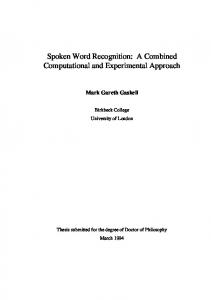
Chapter 2: The “visual world” paradigm In typical psychophysical experiments, the goal is to isolate a component of behavior to the greatest possible extent. Almost always, this entails removing the task from a naturalistic context. While a great deal has been learned about perception and cognition with this classical approach, it leaves open the possibility that perception and cognition in natural, ongoing tasks may operate under very different constraints. Recently, a handful of researchers have begun examining visual and motor performance in more natural tasks (e.g., Hayhoe, 2000; Land and Lee, 1994; Land, Mennie and Rusted, 1998; Ballard et al., 1997). The key methodological advance that has allowed this change in focus is the development of head-mounted eye trackers that allow relatively unrestricted body movements, and thus can provide a continuous measure of visual performance during natural tasks. In this chapter, we will describe the eye tracker used in the experiments described in the following chapters. Then, we will briefly review its use in the study of vision, and the adaptation of this technique for studying language processing. The apparatus and rationale An Applied Science Laboratories (ASL) 5000 series head-mounted eye tracker was used for the first two experiments reported here. An SMI EyeLink, which operates on similar principles, was used for the last three experiments. The tracker consists mainly of two cameras mounted on a headband. One provides a near-infrared image of the eye sampled at 60 Hz. The pupil center and first Purkinje reflection are tracked by a combination of hardware and software in order to provide a constant measure of the position of the eye relative to the head. The second camera (the “scene” camera) is aligned with the subject’s line of sight (see Figure 2.1). Because it is mounted on the headband and moves when the subject’s head does, it remains aligned with the subject’s line of sight. Therefore, the position of the eye relative to

11

the head can be mapped onto scene camera coordinates through a calibration procedure. The ASL software/hardware package provides a cross hair indicating point-of-gaze superimposed on a videotape record from the scene camera. Accuracy of this record (sampled at video frame rates of 30 Hz) is approximately 1 degree over a range of +/- 25 degrees. An audio channel is recorded to the same videotape. Using a Panasonic HI-8 VCR with synchronized sound and video, data is coded frame-byframe, and eye position is recorded with relation to visual and auditory stimuli. Visual stimuli are displayed on a computer screen, and fluent speech is either spoken (in the case of the Allopenna, Magnuson and Tanenhaus, 1998, study we will review below) or played to the subject over headphones using standard Macintosh PowerPC D-to-A facilities. The rationale for using eye movements to study cognition is that eye movements are typically fairly automatic, and are under limited conscious control. On average, we make 2-3 eye movements per second (although this can vary widely depending on task constraints; Hayhoe, 2000), and we are unaware of most of them. Furthermore, saccades are ballistic movements; once a saccade is launched, it cannot be stopped. Given a properly constrained task, in which the subject must perform a visually-guided action, eye movements can be given a functional interpretation. If they follow a stimulus in a reliable, predictable fashion with minimal lag,2 they can be interpreted as actions based on underlying decision mechanisms. Although there is evidence that eye movements in unconstrained, free-viewing linguistics tasks are highly correlated with linguistic stimuli (Cooper, 1974), all of the experiments in this proposal will use visual-motor tasks in order to avoid the pitfalls of interpreting unconstrained tasks (see Viviani, 1990).

2

We take 200 ms to be a reasonable estimate of the time required to plan and launch a saccade in this task, given that the minimum latency is estimated to be between 150 and 180 ms in simple tasks (e.g., Fischer, 1992; Saslow, 1967), whereas intersaccadic intervals in tasks like visual search fall in the range of 200 to 300 ms (e.g., Viviani, 1990).

12

Subject's view (from scene camera on helmet)

ASL/ PC VCR

Figure 2.1: Eye tracking methodology.

Eye camera

13

Vision and eye movements in natural, ongoing tasks Models of visuo-spatial working memory have typically been concerned with the limits of human working memory. Results from studies pushing working memory to its limits have led to the proposal of modality-specific “slave” systems that provide short-term stores. Usually, it is assumed that there are at least two such stores: the articulatory loop, which supports verbal working memory, and the visuo-spatial scratchpad (Baddeley and Hitch, 1974) or “inner scribe” (Logie, 1995), which supports visual working memory. Recent research by Hayhoe and colleagues was designed to complement such work with studies of how capacity limitations constrain performance in natural, ongoing tasks carried out without added time or memory pressures. The prototypical task they use is block-copying (see Figure 2.2). Participants are presented with a visual display (on a computer monitor or on a real board) that is divided into three areas. The model area contains a pattern of blocks. The participant’s task is to use blocks from the resource area to construct a copy of the model pattern in the workspace. Eye and hand position are measured continuously as the participant performs the task. The task is to use blocks displayed in the resource (right monitor) to build a copy of the model (center) in the workspace (left). The arrows and numbers indicate a typical fixation pattern during block copying. The participant fixates the current block twice. At fixation 2, the participant picks up the dark gray block. After fixation 4, the participant drops the block.

Workspace

4

Model

1 3 Figure 2.2: The block-copying task.

Resource

2

14

Note that the task differs from typical laboratory tasks in several ways. First, it is closer to natural, everyday tasks than, e.g., tests of iconic memory or recognition tasks. Second, as a natural task, it extends over a time scale of several seconds. Third, the eye and hand position measures allow one to examine performance without interrupting the ongoing task; that is, the time scale and dependent measures allow one to examine instantaneous performance at any point, but also to have a continuous measure of performance throughout an entire, uninterrupted natural task. Studies using variants of the block-copying task have revealed that information such as gaze and hand locations can be used as pointers to reduce the amount of information that must be internally represented (e.g., Ballard, Hayhoe, and Pelz, 1995). These pointers index locations of task-relevant information, and are called deictic codes (Ballard, Hayhoe, Pook, and Rao, 1997). In several variants of the block-copying task, the same key result has been replicated. Rather than committing even a small portion of a model pattern to memory, participants work with one component at a time, and typically fixate each model component twice. First, participants fixate a model component and then scan the resource area for the appropriate component and fixate it. The hand moves to pick up the component. Then, a second fixation is made to the same model component as on the previous model fixation. Finally, participants fixate the appropriate location in the workspace and move the component from the resource area to place it in the workspace. If we divide the data into fixation-action sequences each time an object is dropped in the workspace, this model-pickup-model-drop sequence is the most often observed (~45%, with the next most frequent pattern being pickup-model-drop, which accounts for ~25% of the sequences; model-pickup-drop and pickup-drop each account for ~10% of the sequences, with most of the remaining, infrequent patterns involving multiple model fixations between drops; thus, the majority of fixation sequences involve at least one model fixation per component, with an average of nearly two model fixations per component).

15

Given such a simple task, why don’t participants encode and work on even two or three components between model fixations, which would be well within the range of short-term memory capacity? Ballard et al. (1997) have proposed that memories for motor signals and eye or hand locations provide a more efficient mechanism than could be afforded by a purely visual, unitary, imagistic representation. In the block-copying paradigm, participants seem to encode simple properties one at a time, rather than encoding complex representations of entire components. For example, a fixation to a model component could be used to encode the block’s color, and its location within the pattern. This might require encoding not just the block’s color, but also the colors of its neighbors (which would indicate its relative location). Alternatively, the block’s color and the signal indicating the fixation coordinates could be encoded. With the color information, a fixation can be made to the resource area to locate a block for the copy. The fixation coordinates could serve as a pointer to the block’s location in the model (and all potential information available at that location). Next, a saccade can be made back to the fixation coordinates, and the information necessary for placing the picked-up block in the workspace can be encoded. Note that in the copying task, the second fixation is typically made back to exactly the same place in the model. Why can’t the information that allows the participant to fixate the same location be used to place the picked-up block in the correct place in the workspace? Because that information is about an eye position – the pointer – not about the relative location of the block in the pattern. The fixation coordinates act as a pointer in the sense of the computer programming term: a small information unit that represents a larger information unit simply by encoding its location. Thus, very little information need be encoded internally at a given moment. Perceptual pointers allow us to reference the external world and use it as memory, in a just-in-time fashion. This hypothesis was inspired in part by an approach in computer vision that greatly reduced the complexity of representations needed to interact with the world. On the active or animate vision view (Bajcsy, 1985; Brooks,

16

1986; Ballard, 1991), much less complex representations of the world are needed when sensors are deployed (e.g., camera saccades are made) in order to sample the world frequently, in accord with task demands. Hayhoe, Bensinger and Ballard (1998) reported compelling evidence for the pointer hypothesis in human visuo-motor tasks. As participants performed the blockcopying task at a computer display, the color of an unworked model block was sometimes changed during saccades to the model area (when the participant would be functionally blind for the approximately 50 ms it takes to make a saccadic eye movement). The color changes occurred either after a drop in the workspace (before pickup), or after a pickup in the resource area (after pickup). Participants were unaware of the majority of color changes, according to their verbal reports. However, fixation durations revealed that performance was affected. Fixation durations were slightly, but not reliably, longer (+43 ms) when a color change occurred before pickup compared to a control when no color change occurred. When the color change occurred after pickup, fixation durations were reliably longer (+103 ms) than when no change occurred. How do these results support the pointer hypothesis? Recall that the most frequent fixation pattern was model-pickup-model-drop. When the change occurs after pickup -- just after the participant has picked up a component from the resource area and is about to fixate the corresponding model block again -- there is a relatively large effect on performance. When the color change occurs before pickup -- just after a participant has finished adding a component to the workspace -- there is a relatively small effect. At this stage, according to the pointer hypothesis, color information is no longer relevant; what had been encoded for the preceding pickup and drop can be discarded, and this is reflected in the small increase in fixation duration. Bensinger (1997) explored various alternatives to this explanation. He found that the same basic results hold when: (a) participants can pick up as many components as they like (in which case they still make two fixations per component, but with sequences like model-pickup, model-pickup, model-drop, model-drop), (b)

17

images of complex natural objects are used rather than simple blocks, or (c) the model area is only visible when the hand is in the resource area (in which case the number of components being worked on drops when participants can pick up as many components as they want, so as to minimize the number of workspace locations to be recalled when the model is not visible). Language-as-product vs. language-as-action The studies we just reviewed reveal a completely different perspective of visual behavior than classical methods for studying visuo-spatial working memory. The discovery that multiple eye movements can substitute for complex memory operations might not have emerged using conventional paradigms. Language research also relies largely on classical, reductionist tasks, on the one hand, and, on the other, on more natural tasks (such as cooperative dialogs) that do not lend themselves to fine-grained analyses. Clark (1992) refers to this as the distinction between languageas-product and language-as-action traditions. In the language-as-product tradition, the emphasis is on using clever, reductionist tasks to isolate components of hypothesized language processing mechanisms. The benefit of this approach is the ability to make inferences about mechanisms due to differences in measures such as response time or accuracy as a function of minimal experimental manipulations. The cost is the potential loss of ecological validity; as with vision, it is not certain that language-processing behavior observed in artificial tasks will generalize to natural tasks. In the language-as-action tradition, the emphasis is on language in natural contexts, with the obvious benefit of studying behavior closer to that found “in the wild.” The cost is the difficulty of making measurements at a fine enough scale to make inferences about anything but the macrostructure of the underlying mechanisms. The head-mounted eye-tracking paradigm provides the means of bringing the two language research traditions closer together. As in the vision experiments, subjects can be asked to perform relatively natural tasks. Eye movements provide a

18

continuous, fine-grained measure of performance, which allows (specially designed) natural tasks to be analyzed at an even finer level than conventional measures from the language-as-product tradition. To illustrate this, we will briefly review one study of spoken word recognition using this technique (known as “the visual world paradigm”). The microstructure of lexical access: Cohorts and rhymes Allopenna, Magnuson and Tanenhaus (1998) extended some previous work using this paradigm (Tanenhaus et al., 1995) to resolve a long-standing difference in the predictions of two classes of models of spoken word recognition. “Alignment” models (e.g., Marslen-Wilson’s Cohort model [1987] or Norris’ Shortlist model [1994]) place a special emphasis on word onsets to solve the segmentation problem – that is, finding word boundaries. Marslen-Wilson and Welsh (1978) proposed that an optimal solution would be, starting from the onset of an utterance, to consider only those word forms consistent with the utterance so far at any point. Given the stimulus beaker, at the initial /b/, all /b/-initial word forms would form the cohort of words accessed as possible matches to the input. As more of the stimulus is heard, the cohort is whittled down (from /b/-initial to /bi/-initial to /bik/-initial, etc.) until a single candidate remains. At that point, the word is recognized, and the process begins again for the next word.3 In its revised form, as with the Shortlist model, Cohort maintains its priority on word onsets (and thus constrains the size of the cohort) in an activation framework by employing bottom-up inhibition. Lower-level units have bottom-up inhibitory connections to words that do not contain them (tripling, on average, the number of connections to each word in an architecture where phonemes connect to words, compared to an architecture like TRACE’s, where there are only excitatory bottom-up connections). In contrast to alignment models’ emphasis on word onsets, continuous activation models like TRACE (McClelland and Elman, 1986) and NAM/PARSYN 3

In cases where there ambiguity remains, the Cohort model’s selection and integration mechanisms complete the segmentation decision.

19

(Luce and Pisoni, 1998; Luce et al., in press) are not designed to give priority to word onsets. Words can become active at any point due to similarity to the input. The advantage for items that share onsets with the input (which we will refer to as cohort items, or cohorts) is still predicted, because active word units inhibit all other word nodes. As shown in Figure 2.3, cohort items become activated sooner than, e.g., rhymes. Thus, cohort items (as well as the correct referent) inhibit rhymes and prevent them from becoming as active as cohorts, despite their greater overall similarity. Still, substantial rhyme activation is predicted by continuous activation models, whereas in alignment models, an item like ‘speaker’ would not be predicted to be activated by an input of ‘beaker.’ Until recently, there was ample evidence for cohort activation (e.g., MarslenWilson and Zwitserlood, 1989), but there was no clear evidence for rhyme activation. For example, weak rhyme effects had been reported in cross-modal and auditoryauditory priming (Connine, Blasko and Titone, 1993; Andruski et al., 1994) when the rhymes differed by only one or two phonetic features. The hints of rhyme effects left open the possibility that conventional measures were simply not sensitive enough to detect the robust, if relatively weak, rhyme activation predicted by models like TRACE.4 Encouraged by the ability of the visual world paradigm to measure the time course of activation among cohort items (Tanenhaus et al., 1995), Allopenna et al. (1998) designed an experiment to take another look at rhyme effects.

4

This is especially true when null or weak results come from mediated tasks like cross-modal priming, where the amount of priming one would expect was not specified by any explicit model. Presumably, weak activation in one modality would result in even weaker activation spreading to the other.

20

Figure 2.3: Activations over time in TRACE.

An example of the task the subject performed in our first experiment was shown in Figure 2.1. The subject saw pictures of four items on each trial. The subjects’ task was to pick up an object in response to a naturally spoken instruction (e.g., “pick up the beaker”) and then place it relative to one of the geometric figures on the display (“now put it above the triangle”). On most trials, the names of the

21

objects were phonologically unrelated (to the extent that no model of spoken word recognition would predict detectable competition among them). On a subset of critical trials, the display included a cohort and/or rhyme to the referent. We were interested in the probability that subjects would fixate phonologically similar items compared to unrelated items as they recognized the last word in the first command (e.g., “beaker”).

Figure 2.4: Fixation proportions from Experiment 1 in Allopenna et al. (1998).

22

Fixation probabilities averaged over 12 subjects and several sets of items are shown in Figure 2.4. The data bear a remarkable resemblance to the TRACE activations shown in Figure 2.3. However, those activations are from an open-ended recognition process, and cannot be compared directly to fixation probabilities for two reasons. First, probabilities sum to one, which is not a constraint on TRACE activations. (Note that the fixation proportions in Figure 2.4 do not sum to one because subjects begin each trial fixating a central cross; the probability of fixating this cross is not shown.) Second, subjects could fixate only the items displayed during each trial. We needed a linking hypothesis to relate TRACE activations to behavioral data. We addressed these two problems by converting activations to predicted fixation probabilities using a variant of the Luce choice rule (Luce, 1959). The basic choice rule is:

Si = e ai k Pi =

Si ∑Sj

(1) (2)

Where Si is the response strength of item i, given its activation, ai, and k, a constant5 that determines the scaling of strengths (large values increase the advantage for higher activations). Pi is the probability of choosing i; it is simply Si normalized with respect to all items’ (1 to j) strengths (at each cycle of activation). One problem with applying the basic choice rule to activations is that given j possible choices, when the activation of all j items is 0, each would have a response probability of 1/j. To rectify this, a scaling factor was computed for each cycle of activations: ∆t =

5

max(at ) max(a overall )

(3)

Actually, a sigmoid function was used in place of a constant in Allopenna et al. (1998). This improves the fit somewhat; see Allopenna et al. for details.

23

This scaling factor (the maximum activation at time t over the maximum activation observed in response to the current stimulus over an arbitrary number of cycles) made response probabilities range from 0 to 1, where 0 indicated all activations were at 0 and 1 indicates that one item was active and equal to the peak activation. The second modification to the choice rule was that only items visually displayed entered into the response probability equations, given that subjects could only choose among those items. Thus, activations were based on competition within the entire lexicon (the standard 230-word TRACE lexicon augmented with our items, and their neighbors, for a total of 268 items), but choices were assumed only to take into account visible items. Note that this fact could have been incorporated in many different ways. For example, the implementation of TRACE we used allows a topdown bias to be applied to specific items, which would change the dynamics of the activations themselves. The post-activation selection bias we used carries the implicit assumption that competition in the lexicon is protected from top-down biases from other modalities. As we will discuss in Chapter 4, this assumption should be tested explicitly. However, the method we used provided an exceptionally good fit to the data. Predicted fixation probabilities are shown in Figure 2.5. To measure the fit, RMS error and correlations were computed. RMS values for the referent, cohort, and rhyme were .07, .03 and .01, respectively. r2 values were .98, .90, and .87. Note that the results also support TRACE over the NAM, in that cohort items compete more strongly than rhymes. In the NAM, rhymes are predicted to be more likely responses than cohorts due to their greater similarity to the referent. Thus, TRACE provides a better fit to data because it incorporates the temporal constraints on spoken language perception: evidence accumulates in a “left-to-right” manner. The NAM, on the other hand, remains quite useful because it produces a single number for each lexical item that is fairly predictive of the difficulty subjects will have recognizing it.

24

Figure 2.5: TRACE activations converted to response probabilities.

The Allopenna et al. (1998) study demonstrates how a sufficiently sensitive, continuous and direct measure can address questions of microstructure. The experiments reported here extend this work to even finer-grained questions regarding the time course of neighborhood density (Experiments 1 and 2), appropriate similarity metrics for spoken words (Experiments 1-3), and the time course of the integration of

25

top-down information during acoustic-phonetic processing (Experiment 5). We extend the methodology to achieve more precise control over stimulus characteristics (by instantiating levels of characteristics in artificial lexicons), and by examining important control issues (to what degree effects in the visual world paradigm are controlled by the displayed objects [Experiments 2 and 5], and whether the native lexicon intrudes on processing items in a newly-learned artificial lexicon [Experiment 4]).

26

Chapter 3: Studying time course with an artificial lexicon As the sound pattern of a word unfolds over time, multiple lexical candidates become active and compete for recognition. The recognition of a word depends not only on properties of the word itself (e.g., frequency of occurrence; Howes, 1954), but also on the number and properties of phonetically similar words (Marslen-Wilson, 1987; 1993), or neighbors (e.g., Luce and Pisoni, 1998). The set of activated words is not static, but changes dynamically as the signal is processed. Models of spoken word recognition (SWR) must take into account the characteristics of dynamically changing processing neighborhoods in continuous speech (e.g., Gaskell and Marslen-Wilson, 1997; Norris, 1994). Recent methodological advances using an eye-tracking measure allow for direct assessment of the time course of SWR at a fine temporal grain (e.g., Allopenna, Magnuson and Tanenhaus, 1998). However, the degree to which these, and other more traditional methods, can be used to evaluate hypotheses about the dynamics of processing neighborhoods depends on how precisely the distributional properties of words in the lexicon (such as word frequency and number of potential competitors) can be controlled. Artificial linguistic materials have been used to study several aspects of language processing with precise control over distributional information (e.g., Braine, 1963; Morgan, Meier and Newport, 1987; Saffran, Newport and Aslin, 1996). The present chapter introduces and evaluates a paradigm that combines the eye-tracking measure with an artificial lexicon, thereby revealing the time course of SWR while word frequency and neighborhood structure are controlled with a precision that could not be attained in a natural-language lexicon. In the paradigm we developed, participants learn new “words” by associating them with novel visual patterns, which enabled us to examine how precisely controlled distributional properties of the input affect processing and learning. This is an important advantage of an artificial lexicon because on-line SWR in a natural-language lexicon is difficult to study during the

27

process of acquisition, particularly when the goal is to determine how word learning is affected by the structure of lexical neighborhoods. The usefulness of the artificial lexicon approach depends crucially on the degree to which SWR in a newly learned lexicon is similar to SWR in a mature lexicon. We address this question by using the same eye movement methods that have been used to study natural-language lexicons, and comparing the results obtained with an artificial lexicon to related studies using real words. Eye movements to objects in visual displays during spoken instructions provide a remarkably sensitive measure of the time course of language processing (Cooper, 1974; Tanenhaus, Spivey-Knowlton, Eberhard and Sedivy, 1995; for a review, see Tanenhaus, Magnuson, and Chambers, in preparation), including lexical activation (Allopenna, Magnuson and Tanenhaus, 1998; Dahan, Magnuson and Tanenhaus, in press; Dahan, Magnuson, Tanenhaus and Hogan, in press; for a review, see Tanenhaus, Magnuson, Dahan, and Chambers, in press). Allopenna et al. (1998) monitored eye movements as participants followed instructions to click on and move one of four objects displayed on a computer screen (see Figure 2.1 in Chapter 2) with the computer mouse (e.g., “Look at the cross. Pick up the beaker. Now put it above the square.”). The probability of fixating each object as the target word was heard was hypothesized to be closely linked to the activation of its lexical representation. The assumption providing the link between lexical activation and eye movements is that the activation of the name of a picture affects the probability that a participant will shift attention to that picture and fixate it. On critical trials, the display contained a picture of the target (e.g., beaker), a picture whose name rhymed with the target (e.g., speaker), and/or a picture that had the same onset as the target (e.g., beetle, called a “cohort” because items sharing onsets are predicted to compete by the Cohort model; e.g., Marslen-Wilson, 1987), as well as unrelated items (e.g., carriage) that provided baseline fixation probabilities. Figure 2.4 (in Chapter 2) shows the proportion of fixations over time to the visual referent of the target word, its cohort and rhyme competitors, and an unrelated

28

item. The proportion of fixations to referents and cohorts began to increase 200 ms after word onset. We take 200 ms to be a reasonable estimate of the time required to plan and launch a saccade in this task, given that the minimum latency is estimated to be between 150 and 180 ms in simple tasks (e.g., Fischer, 1992; Saslow, 1967), whereas intersaccadic intervals in tasks like visual search fall in the range of 200 to 300 ms (e.g., Viviani, 1990). Thus, eye movements proved sensitive to changes in lexical activation from the onset of the spoken word and revealed subtle but robust rhyme activation which had proved elusive with other methods. Although competition between cohort competitors was well-established (for a review see Marslen-Wilson, 1987), rhyme competition was not. Weak rhyme effects had been found in cross-modal and auditory-auditory priming, but only when rhymes differed by one or two phonetic features in the initial segment (Andruski, Blumstein, and Burton, 1994; Connine, Blasko, and Titone, 1993; Marslen-Wilson, 1993). The rhyme activation found by Allopenna et al. (1998) favored continuous activation models, such as TRACE (McClelland and Elman, 1986) or PARSYN (Luce, Goldinger, and Auer, 2000), in which late similarity can override detrimental effects of initial mismatches, over models such as the Cohort model (Marslen-Wilson, 1987, 1993) or Shortlist (Norris, 1994) in which bottom-up inhibition heavily biases the system against items once they mismatch. Dahan, Magnuson and Tanenhaus (2001) used the eye-movement paradigm to measure the time course of frequency effects and demonstrated that frequency affects the earliest moments of lexical activation, thus disconfirming models in which frequency acts as a late, decision-stage bias (e.g., Connine, Titone, and Wang, 1993). When a picture of a target word, e.g., bench, was presented in a display with pictures of two cohort competitors, one with a higher frequency name (bed) and one with a lower frequency name (bell), initial fixations were biased towards the high frequency cohort. When the high- and low-frequency cohorts were used as targets in displays in which all items had unrelated names, the fixation time course to pictures with higher frequency names was faster than for pictures with lower frequency names. This

29

demonstrated that frequency effects in the paradigm do not depend on the relative frequencies of displayed items, and that the visual display does not reduce or eliminate frequency effects, as in closed-set tasks (e.g., Pollack, Rubenstein and Decker, 1959; Sommers, Kirk and Pisoni, 1997). In the present research, the position of overlap with the target was manipulated by creating cohort and rhyme competitors, frequency was manipulated by varying amount of exposure to words, and neighborhood density was manipulated by varying neighbor frequency. Four questions were of primary interest. First, would participants learn the artificial lexicon quickly enough to make extensions of the paradigm feasible? Second, is rapid, continuous processing a natural mode for SWR, or does it arise only after extensive learning? Third, would we find the same pattern of effects observed with real words (cohort and rhyme competition, frequency effects)? Fourth, do effects in this paradigm depend on visual displays, or is recognition of a word influenced by properties of its neighbors, even when their referents are not displayed? This would demonstrate that the effects are primarily driven by SWR processes. Experiment 1 Method Participants. Sixteen students at the University of Rochester who were native speakers of English with normal hearing and normal or corrected-to-normal vision were paid $7.50 per hour for participation.

Materials. The visual stimuli were simple patterns formed by filling eight randomly-chosen, contiguous cells of a four-by-four grid (see Figure 3.1). Pictures were randomly mapped to words.6 The artificial lexicon consisted of four 4-word sets

6

Two random mappings were used for the first eight participants, with four assigned to each mapping. A different random mapping was used for each of the eight subjects in the second group. ANOVAs using group as a factor showed no reliable differences, so we have combined the groups.

30

of bisyllabic novel words, such as /pibo/, /pibu/, /dibo/, and /dibu/.7 Mean duration was 496 ms. Each word had an onset-matching (cohort) neighbor, which differed only in the final vowel, an onset-mismatching (rhyme) neighbor, which differed only in its initial consonant, and a dissimilar item which differed in the first and last phonemes. The cohorts and rhymes qualify as neighbors under the “short-cut” neighborhood metric of items differing by a one-phoneme addition, substitution or deletion (e.g., Newman, Sawusch, and Luce, 1997). A small set of phonemes was selected in order to achieve consistent similarity within and between sets. The consonants /p/, /b/, /t/, and /d/ were chosen because they are among the most phonetically similar stop consonants. The first phonemes of rhyme competitors differed by two phonetic features: place and voicing. Transitional probabilities were controlled such that all phonemes and combinations of phonemes were equally predictive at each position and combination of positions. A potential concern with creating artificial stimuli is interactions with real words in the participants’ native lexicons. While Experiment 4 addresses this issue explicitly, none of the stimuli in this study would fall into dense English neighborhoods (9 words had no English neighbors; 5 had 1 neighbor, with log frequencies between 2.6 and 5.8; 2 had 2 neighbors, with summed log frequencies of 4.1 and 5.9). Furthermore, even if there were large differences, these would be unlikely to control the results, as stimuli were randomly assigned to frequency categories in this experiment, as will be described shortly. The auditory stimuli were produced by a male native speaker of English in a sentence context (“Click on the pibo.”). The stimuli were recorded to tape, and then digitized using the standard analog/digital devices on an Apple Macintosh 8500 at 16 bit, 44.1 kHz. The stimuli were converted to 8 bit, 11.127 kHz (SoundEdit format) for use with the experimental control software, PsyScope 1.2 (Cohen, MacWhinney, Flatt and Provost, 1993). 7

The other items were /pota/, /poti/, /dota/, /doti/; /bupa/, /bupi/, /tupa/, /tupi/; and /bado/, /badu/, /tado/, /tadu/.

31

Figure 3.1: Examples of 2AFC (top) and 4AFC displays from Experiments 1 and 2.

Procedure. Participants were trained and tested in two 2-hour sessions on consecutive days. Each day consisted of seven training sessions with feedback and a testing session without feedback. Eye movements were tracked during the testing session. The structure of the training sessions was as follows. First, a central fixation cross appeared on the screen. The participant then clicked on the cross to begin the trial. After 500 ms, either two shapes (in the first three training sessions) or four shapes (in the rest of the training sessions and the tests) appeared (see Figure 3.1).

32

Participants heard the instruction, “Look at the cross.”, through headphones 750 ms after the objects appeared. As instructed prior to the experiment, participants fixated the cross, then clicked on it with the mouse, and continued to fixate the cross until they heard the next instruction. 500 ms after clicking on the cross, the spoken instruction was presented (e.g., “Click on the pibu.”). When participants responded, all of the distractor shapes disappeared, leaving only the correct referent. The name of the shape was then repeated. The object disappeared 500 ms later, and the participant clicked on the cross to begin the next trial. The testing session was identical to the four-item training, except that no feedback was given. During training, half the items were presented with high frequency (HF), and half with low frequency (LF). Half of the eight HF items had LF neighbors (e.g., /pibo/ and /dibu/ might be HF, and /pibu/ and /dibo/ would be LF), and vice-versa. The other items had neighbors of the same frequency. Thus, there were four combinations of word/neighbor frequency: HF/HF, LF/LF, HF/LF, and LF/HF. Each training session consisted of 64 trials. HF names appeared seven times per session, and LF names appeared once per session. Each item appeared in six test trials: one with its onset competitor and two unrelated items, one with its rhyme competitor and two unrelated items, and four with three unrelated items (96 total). Eye movements were monitored using an Applied Sciences Laboratories E4000 eye tracker, which provided a record of point-of-gaze superimposed on a video record of the participant's line of sight. The auditory stimuli were presented binaurally through headphones using standard Macintosh Power PC digital-to-analog devices and simultaneously to the HI-8 VCR, providing an audio record of each trial. Trained coders (blind to picture-name mapping and trial condition) recorded eye position within one of the cells of the display at each video frame.

33

Figure 3.2: Day 1 test (top) and Day 2 test (bottom) from Experiment 1.

34

Results A response was scored as correct if the participant clicked on the named object with the mouse. Participants were close to ceiling for HF items in the first test, but did not reach ceiling for LF items until the end of the second day (see Table 1). Eye position was coded for each frame on the video tape record beginning 500 ms before target onset and ending when the participant clicked on a shape. The second day's test was coded for all subjects. The first day's test was coded only for the second group of eight subjects (see footnote 6). In order not to overestimate competitor fixations, only correct trials were coded.

Cohort and rhyme effects. Figure 3.2 shows the proportion of fixations to cohort, rhyme and unrelated distractors8 in 33 ms time frames (video sampling rate: 30 Hz), averaged across all frequency and neighbor (cohort or rhyme) conditions for the test on Day 1 (n = 8) and Day 2 (n = 16). The overall pattern is strikingly similar to the pattern Allopenna et al. (1998) found with real words (see Figure 2.4 in Chapter 2). On both days cohorts and rhymes were fixated more than unrelated distractors. The cohort and target proportions separated together from the unrelated baseline. After a slight delay (more apparent on day two), the fixation probability of the rhyme separated from baseline. Eye movements were more closely time-locked to speech than it appears in the figures. Allowing for the estimated 200 ms it takes to plan and launch a saccade, the earliest eye movements were being planned almost immediately after target onset. Since the average target duration was 496 ms, eye movements in about the first 700 ms were planned and launched prior to target offset.

8 Fixation probabilities for unrelated items represent the average fixation probability to all unrelated items.

35

Figure 3.3: Cohort effects on Day 2 in Experiment 1.

36

Note that the slope of the target fixation probability (derived from a logistic regression) was less than for real words (Day 1: probability increased .0006/msec; Day 2: .0007; real words: .0021; see Figure 2.4 in Chapter 2), and the target probability did not reach 1.0 even 1500 ms after the onset of the target name. Two factors underlie this. First, the stimuli were longer than bisyllabic words like those used by Allopenna et al. because of their CVCV structure. Second, although participants were at ceiling on HF and LF items in the second test (Table 3.1), they were apparently not as confident as we would expect them to be with real words, as indicated by the fact that they made more eye movements than participants in Allopenna et al. (1998): 3.4 per trial on Day 2 vs. 1.5 per trial for real words.

Table 3.1: Accuracy in training and testing in Experiment 1.

Session

Overall

HF

LF

Training 1 (2AFC)

0.728

0.751

0.562

Training 4 (2AFC)

0.907

0.933

0.722

Training 7 (4AFC)

0.933

0.952

0.797

Day 1 Test

0.863

0.949

0.777

Training 8 (4AFC)

0.940

0.960

0.802

Training 11 (4AFC)

0.952

0.965

0.859

Training 14 (4AFC)

0.969

0.977

0.908

Day 2 Test

0.974

0.983

0.964

37

Figure 3.4: Rhyme effects on Day 2 in Experiment 1.

38

Two differences stand out between the results for Days 1 and 2. First, the increased slope for target fixation probabilities on Day 2 reflects additional learning. Second, the rhyme effect on Day 1 appeared to be about as strong as the cohort effect. ANOVAs on mean fixation probabilities9 in the 1500 ms after target onset showed that cohort and rhyme probabilities reliably exceeded those for unrelated items on Day 1 (cohort [.10] vs. unrelated [.04]: F[1,7]=11.0, p < .05; rhyme [.09] vs. unrelated [.05]: F[1,7]=7.2, p < .05), but the cohort and rhyme did not differ from one another (F[1,7]