Myra Spiliopoulou1. Irene Ntoutsi2. 1School of Computer Science. University of Magdeburg. Magdeburg, Germany. {myra,schult}@iti.cs.uni-magdeburg.de.
The MONIC Framework for Cluster Transition Detection ∗ Myra Spiliopoulou1 1
Irene Ntoutsi2
School of Computer Science University of Magdeburg Magdeburg, Germany
{myra,schult}@iti.cs.uni-magdeburg.de
ABSTRACT There is much recent work on detecting and tracking changes in clusters, often based on the study of their spatiotemporal properties. For the many applications where cluster change is relevant, among them customer relationship management, fraud detection and marketing, it is also necessary to provide insights about the nature of change: Is a cluster corresponding to a group of customers simply disappearing or are its members migrating to other clusters? Is a new emerging cluster reflecting a new target group of customers or does it rather consist of existing customers whose preferences shift? To answer such questions, we propose the MONIC framework for modelling and tracking of cluster transitions. Our cluster transition model encompasses changes that involve more than one cluster, thus allowing for insights on cluster change in the whole clustering. Our transition tracking mechanism is not based on the topological properties of clusters, which are only available for some types of clustering, but on the contents of the underlying data stream. We present our first results on monitoring cluster transitions over the ACM digital library.
Keywords Cluster change detection, cluster transitions, data streams, clusters, temporal analysis
1.
INTRODUCTION
In recent years, it has been recognized that the clusters discovered in many real applications are affected by changes in the underlying population of customer transactions, user activities, network accesses or documents. Much of the research in this area has been devoted in adapting the clusters to the changed population, so that they always reflect the current state of the population. Recently, research has ∗A short version of this work appears in the Proceedings of ACM SIGKDD International Conference on Knowledge Discovery and Data Mining(KDD’06)
Yannis Theodoridis2 2
Rene Schult1
Department of Informatics University of Piraeus Piraeus, Greece
{ntoutsi,ytheod}@unipi.gr
expanded to encompass tracing and understanding of the changes themselves, as means of gaining valuable insights on the population and of supporting strategic decisions. In Fig. 1, we visualize the challenge of understanding changes: We depict clusters at four timepoints – they might be user profiles or topics in news. New records are marked with darker points; old records are forgotten, using a time window of size 2. The clusters at each timepoint can be easily seen. It is also apparent that changes have occurred. However, finding the same cluster again, categorizing and tracing the changes upon it is much more challenging: “Did some clusters disappear? Or were they rather absorbed by others? When is a cluster the same and when does it mutate?” In this paper, we propose the MONIC framework for the categorization and tracing of such cluster changes. MONIC takes as input an accumulating data collection, the records of which are subject to ageing, as is typical in data stream applications. The records are clustered at consecutive data points and their evolution is monitored. To this purpose, we first propose a typification of cluster transitions, in which we distinguish between internal transitions that affect the cluster itself and external transitions that concern the cluster with respect to other clusters. For the detection of the transitions, we propose transition indicators incorporated in a transition detection algorithm. Finally, we use the detected transitions to draw conclusions about the temporal properties of clusters and clusterings, such as lifetime and temporal stability. Differently from spatiotemporal clustering methods [1, 15, 18] for cluster evolution, MONIC does not rely on a metric space and on an appropriate trajectory for cluster transition detection. Thus, MONIC is applicable to arbitrary types of clusters and is independent of the clustering algorithm. In Section 2, we discuss relevant research. In Section 3, we introduce a cluster typification and then specify the notions of overlap and matching for clusters derived from different slots of the dataset. Section 4 contains our cluster transition model and transition detection heuristics. In Section 5 we present our first experiments. We conclude our study with a summary and an outlook.
2. RELATED WORK Research relevant to cluster monitoring can be categorized into cluster change detection methods and spatiotemporal clustering. We also discuss methods on the specific subject of topic evolution [11, 13]. We omit methods on the comparison of clusterings [12, 19], because they assume that cluster matching has been already performed and that the clusters
100
90
90
80
80
70
70
60
60
90
80
80
70 60 60 50
50
50 40 40
40
20
40
30
30
30 20
20
20
0 10
10
0
20
40
60
80
100
10 0
10
20
30
40
50
60
70
80
90
0
10
20
30
40
50
60
70
80
90
0
10
20
30
40
50
60
70
80
90
Figure 1: Data records at four timepoints are derived upon the same dataset.
2.1 Methods for Cluster Change Detection Ganti et al. propose the DEMON framework for data evolution and monitoring across the temporal dimension [9]. DEMON focuses on detecting systematic vs. non-systematic changes in data and on identifying the data blocks (along the time dimension) which have to be processed by the miner in order to extract new patterns. However, the emphasis is on updating the knowledge base by detecting changes in data, rather than understanding changes in patterns. Ganti et al. also proposed the FOCUS framework [8], which compares two datasets and computes a deviation measure between them based on the data mining models they induce. Clusters comprise a special case of data mining models: Clusters are non-overlapping regions described through a set of attributes (structure component) and corresponding to a set of raw data (measure component). However, the emphasis is on comparing datasets; understanding how a cluster has evolved inside a new clustering is beyond the scope of FOCUS. The PANDA framework [5] delivers methods for the comparison of simple patterns, which are defined over raw data, e.g. a cluster, and complex patterns, which are defined over other patterns, e.g. a clustering. The distance between two complex patterns is calculated in a bottom–up fashion based on the distances of their component simple patterns. In PANDA, however, the emphasis is on the generic and efficient realization of comparisons between any complex patterns rather than the detection and interpretation of cluster transitions across the time axis. The “Pattern Monitor” (PAM) [4] models patterns as temporal, evolving objects obeying on a model of changes, proposed in [3]. However, PAM focuses mostly on association rules. We built upon this earlier work, especially for the specification of the data considered at each timepoint.
2.2 Spatiotemporal Clustering Neill et al. [15] study the emergence and stability of clusters, observing spatial regions across the time axis. In their approach, no clustering is performed; rather, cluster existence corresponds to negating the homogeneity assumption. The detection process consists of identifying spatial regions that have, for some property, higher counts than expected. The set of regions is static and known in advance. The expected counts are inferred through time series analysis of the past counts. A sliding time window is used to detect changing, emerging and persistent clusters. Yang et al. [18] detect change events upon clusters of scientific data. They study “Spatial Object Association Patterns” (SOAPs), which are graphs of different types, e.g. cliques or stars. A SOAP is characterized by the number
of snapshots in data, where it occurs and the number of instances in a snapshot that adhere to it. With this information, the algorithm detects “formation” and “dissipation” events, as well as cluster “continuation”. Their method is not dedicated to clusters, rather it refers to patterns in general. Aggarwal [1] proposes a dedicated method for the detection and study of cluster changes across the time axis and across spatial dimensions (in a trajectory). Clusters are modeled through kernel functions and their changes as kernel density changes. More specifically, at each spatial location, the kernel density is computed and two estimates of density change are computed, the backward and the forward estimate upon a sliding time window. Their difference is the velocity density of the location. This is generalized over multiple spatial locations as the global evolution coefficient. Aggarwal distinguishes different types of change, with emphasis on (i) the velocity of change and (ii) the locations exhibiting the highest velocity – the epicenters. A particular feature of the model is the identification of the data properties that mostly contribute to change. All approaches of this category operate upon a trajectory and assume that the trajectory does not change: They observe a cluster as a “densification” of the trajectory and then monitor changes in it. Hence, these methods cannot be coupled with arbitrary clustering algorithms, e.g. general purpose hierarchical algorithms 1 or density-based clusterers. Moreover, these methods juxtapose each cluster to the trajectory and cannot trace interferences among clusters, e.g. one cluster absorbing the other. Finally, these methods cannot be applied if the feature space itself changes, e.g. in text stream mining, where features are usually frequent words. Finally, Kalnis et al. [10] propose a special type of cluster change, the “moving cluster”, whose contents may change while its density function remains the same during its lifetime. They find moving clusters by tracing common data records between clusters of consecutive timepoints. MONIC is more general, since it encompasses several cluster transition types, allows for the “ageing” of old objects and does not require that the density function of a moving cluster is invariant.
2.3 Topic Evolution Topic evolution is a subarea of topic detection and tracking [2]. Typically, a topic is a cluster, thus topic evolution is a special case of cluster monitoring. The works most related 1 Hierarchical clustering algorithms use an ultra-metric, so their clusters cannot be studied outside the metric space of the dataset that produced them.
to MONIC are the studies of [13, 11] on text clustering with mixture models: A topic is described by the words dominant to the distribution of the corresponding cluster, i.e. a topic is a cluster label. In [13], the emphasis is on adapting the clusters, while [11] propose topic transition types and build a topic evolution graph, in which transitions are traced. Here transitions refer to changes in the cluster labels rather than the clusters themselves. These methods are appropriate for applications where an intuitive cluster description, such as a topic composed of words, can be extracted and traced over time. This is not feasible for all applications, though. In the general case, the evolution of a cluster’s mean and standard deviation does not provide clues about cluster absorption or splitting. For this reason, MONIC traces cluster transitions by comparing the (weighted) contents of clusters. This allows us to find transitions that cannot be traced by only studying the distribution of the data or other summary information.
3.
CLUSTER MODEL IN MONIC
MONIC models and traces the transitions of clusters built upon an accumulating dataset. Data are collected and clustered at timepoints t1 , . . . , tn , whereupon old data may be subjected to a “data ageing” function that assigns lower weights to all or some of the past records, as is often the case for topic detection and tracking methods [2]. The set of features used for clustering may also change during the period of observation, thus allowing for the inclusion of new features and the removal of obsolete ones. MONIC assumes re-clustering rather than cluster adaptation at each timepoint, so that both changes in existing clusters and new clusters can be monitored. Moreover, transitions can be detected even when the underlying feature space changes, i.e. when cluster adaptation is not possible. To do so, we first specify the notion of “same” cluster or rather cluster “match” across the time axis. Thereafter, we present a set of cluster transitions upon those clusters.
3.1 Clusterings upon Ageing Data A clustering over a dataset can be observed as a partitioning of the dataset into homogeneous groups. We concentrate on “hard clustering”, in which each object belongs to exactly one cluster, as opposed to “soft clustering”, where an object is associated with each cluster by some probability or possibility value. Definition 1 (Clustering). A “clustering” ζ is a partitioning of a dataset D into the partitions X1 , X2 , . . . , Xk called “clusters” such that (a) Xu ∩ Xw = ∅ for all u 6= w, (b) ∪ku=1 Xu = D and (c) some optimization criterion is satisfied, e.g. the members of each cluster are more similar to each other than to members of other clusters. This is a set-theoretic definition of clusters. More elaborate definitions are possible for clusters over a metric space, whose topology can be used to specify proximity of objects. As mentioned in Section 2, MONIC is intended for arbitrary clustering methods. We therefore observe clusters as sets. Def. 1 assumes a complete partitioning of the dataset. Clusterers that ignore outliers are indirectly covered by assuming a preprocessing step that removes outliers.
Definition 2. Let t1 . . . , tn be the sequence of timepoints under observation and let Di , i = 2 . . . , n be the set of data records accumulated from ti−1 until ti , while D1 is the initial dataset, so that Di ∩ Dj = ∅ for i 6= j. A “data ageing function” assigns a weight age(x, ti ) ∈ [0, 1] to data record x at ti for each x ∈ ∪il=1 Dl and for each ti . age : ∪il=1 Dl × {t1 . . . , tn } → [0, 1] The weights assigned by the ageing function determine the impact of each record upon clustering ζi ≡ ζi (∪il=1 Dl , age, ti ). This function covers sliding windows (the weights of records outside the window are zero) but also more elaborate schemes, e.g. [14] which considers re-appearances of each record and assigns higher weights to recurring records.
3.2 Cluster Matching Consider a cluster X discovered at a timepoint ti as part of a clustering ζi . A “cluster transition” is a change effected upon this cluster, when we observe it at a later timepoint tj . The first step in identifying such a transition is the detection of the cluster X in the corresponding clustering ζj – if it is still existent. Hence, we define the notion of (nonsymmetric) “overlap” and of (best) “match” for a cluster, before we proceed with a categorization of cluster transitions. Definition 3 (Cluster overlap). Let ζi , ζj (i 6= j) be two clusterings derived at the timepoints ti , tj (i 6= j) respectively, and let X ∈ ζi , Y ∈ ζj be two clusters. The overlap of X to Y is the normalized sum of the weights of their common records: overlap(X, Y ) =
P age(a, tj ) Pa∈X∩Y x∈X
age(x, tj )
In this definition, the function age() is used to assign weights to the data records, as specified in Def. 2. It can be also extended so as to restrict the computation of overlap only on the cluster’s core points (cf. [7]) by assigning the value of zero to all non-core points of the cluster X under observation. We can now define for each cluster found at a timepoint ti , its best match at a later timepoint tj . Definition 4 (Cluster match). Let X be a cluster in the clustering ζi at timepoint ti and Y be a cluster in the clustering ζj at timepoint tj > ti . Further, let τ ≡ τmatch ∈ [0.5, 1] be a threshold value. Y is “a match for X in ζj subject to τ ”, i.e. Y = matchτ (X, ζj ) if and only if: 1) Y has the maximum overlap to X among all clusters in ζj , i.e. overlap(X, Y ) = maxY ′ ∈ζj {overlap(X, Y ′ )} and 2) overlap(X, Y ) ≥ τ . If there is no such Y ∈ ζj , then matchτ (X, ζj ) = ∅. By Def. 4, ζj can contain at most one match for each cluster in ζi , although the same cluster in ζj can be the match of more than one clusters in ζi . We restrict the threshold τ to the interval [0.5, 1] to stress that a cluster is a match only if it contains at least half of the pivot cluster members (e.g. half of its members, if the members are weighted equally). A tie can then occur only for τ = 0.5. Different tie breakers can be used, choosing e.g. the Y that has the maximum reverse overlap overlap(Y, X) or the Y that is closest to X in size.
4.
CLUSTER TRANSITIONS IN MONIC
In MONIC , a cluster transition at a given timepoint is a change experienced by a cluster that has been discovered at an earlier timepoint. Such a transition may concern the content and the form of the cluster, i.e. be “internal” to it, or it may concern its relationship to the rest of the clustering, i.e. be an “external” transition. We first define these types of transitions and then introduce heuristics that trace them.
4.1 Detection of External Transitions The “external transitions” of cluster X ∈ ζi with respect to clustering ζj at tj > ti are defined in Table 1: A cluster may disappear, be split into multiple clusters, be absorbed by some larger cluster or survive, whereupon internal transitions may occur (more on internal transitions on Section 4.2). According to Table 1, a cluster X ∈ ζi survives in ζj if (a) there is a match for it in ζj subject to τ ≡ τmatch and (b) this match does not cover any further cluster of ζi . If the match covers at least one further cluster in ζi , then X has been absorbed. If no match exists, then a split may have occurred, i.e. the contents of X are in more than one clusters of ζj . In this case, the overlaps must be no less than τsplit (obviously: τsplit < τmatch ), to prevent degenerate cases. Moreover, all those clusters together must form a match for X. If none of these cases occur, then X has disappeared. All but the last transitions in Table 1 refer to changes of a given cluster. Emerging clusters are detected after tracing all external transitions for each cluster in ζi : Clusters in ζj that are not the result of an external transitions can be considered as “emerged clusters”. In Fig. 2, we present our transition detector. For the clusters in clustering ζi of ti (ζ i in the Figure), it detects their external transitions on clustering ζ j ≡ ζj of tj > ti . For each cluster X ∈ ζi , the detector performs some initializations (the variables are explained later) and then computes the overlap of X to each cluster of ζj (line 5). The detector first looks for clusters in ζj that match X (lines 5– 8). In line 7, the best match for X is selected, according to some tie breaking criterion, as already discussed after Def. 4. So, each cluster in ζi has at most one survival candidate. If no survival exists for the X cluster, clusters overlapping with it for more than τsplit < τmatch are found (lines 10–12). If neither hold, then X is marked as disappeared (lines 15–16). The case of cluster split detection involves building a list of split candidate clusters (line 11). As specified in Table 1, these clusters, when taken together, must form a match for cluster X. The operation of “taking the clusters together” (line 12) currently refers to the set union of the records, i.e. weights are not considered for the moment. However, weights are still considered in the overlap test performed at line 18. If this test succeeds, cluster X is marked as split (line 20), otherwise it is marked as disappeared (line 22). The cases of absorption and survival are initially treated together: ζi clusters and their survival candidates are added to a list of absorptions and survivals (line 24). When all ζi clusters are processed, this list is completed (line 26). Then, for each ζj cluster Y , the detector extracts from this list all ζi clusters for which Y is a survival candidate (line 28). If this sublist contains more than one clusters, then these have been absorbed by Y : They are marked as such (lines 30–31) and removed from the original list (line 32). Otherwise, the single member of the sublist is a cluster X that has survived
1 FOR X ∈ ζ i 2 splitCandidates = splitUnion = ∅; 3 survivalCandidate = NULL; 4 FOR Y ∈ ζ j 5 Mcell = overlap(X,Y); 6 IF Mcell ≥ τ THEN 7 IF g(X,Y) > g(X,survivalCandidate) 8 survivalCandidate = Y; 9 ENDIF 10 ELSEIF Mcell ≥ τ split THEN 11 splitCandidates += Y; 12 splitUnion = splitUnion ∪ Y ; 13 ENDIF 14 ENDFOR 15 IF survivalCandidate == NULL OR splitCandidates == ∅ 16 THEN deadList += X; // X → ⊙ 17 ELSEIF splitCandidates 6= ∅ THEN 18 IF overlap(X,splitUnion) ≥ τ THEN 19 FOR Y ∈ splitCandidates 20 splitList += (X,Y); ⊂ 21 ENDFOR // X → splitCandidates 22 ELSE deadList += X; // X → ⊙ 23 ENDIF 24 ELSE Absorptions˙Survivals += (X,survivalCandidate); 25 ENDIF 26 ENDFOR 27 FOR Y ∈ ζ j 28 absorptionCandidates = makeList(Absorptions˙Survivals,Y); 29 IF cardinality(absorptionCandidates) > 1 THEN 30 FOR X ∈ absorptionCandidates ⊂ 31 absorbtionList += (X,Y); // X → Y 32 Absorptions˙Survivals -= (X,Y); 33 ENDFOR 34 ELSEIF absorptionCandidates == X THEN 35 survivalList += (X,Y); // X → Y 36 Absorptions˙Survivals -= (X,Y); 37 ENDIF 38 ENDFOR
Figure 2:
Detector of external transitions
as Y (line 35). Again, the original list is updated (line 36). Several improvements of this base algorithm are possible. First, instead of computing the overlap for each pair of clusters (line 5), MONIC computes the contingency matrix M of the overlap values and retrieves the appropriate cell M cell, whenever the overlap of two clusters is needed. Furthermore, split detections (lines 12, 18) can be performed more effectively, if one observes that two clusters in ζj cannot have common members. Then, the split test can be computed from the individual intersection values in M because:
X p
a∈X∩(∪u=1 Yu )
age(a, tj ) =
p X X
age(a, tj )
u=1 a∈X∩Yu
Thus, the complexity of the detector is O(K 2 ) for K = max{|ζi |, |ζj |}, once the contingency matrix M is computed.
4.2 Detection of Internal Transitions Survived clusters may undergo internal changes, e.g. shrink or expand. In Table 2, we have grouped the internal transitions as changes in size, compactness and location. The transitions inside a group are mutually exclusive, but transitions of different groups can be combined. For example, a
Transition the cluster survives the cluster is split into multiple clusters the cluster is absorbed the cluster disappears a new cluster has emerged
Notation X →Y ⊂ X → {Y1 , . . . , Yp } ⊂
X →Y X→⊙ ⊙→Y
Indicator Y = matchτ (X, ζj ) AND 6 ∃Z ∈ ζi \ {X} : Y = matchτ (Z, ζj ) (∀u = 1 . . . p : overlap(X, Yu ) ≥ τsplit ) ∧ overlap(X, ∩pu=1 Yu ) ≥ τ ∧ (6 ∃Y ∈ ζj \ {Y1 . . . , Yp } : overlap(X, Y ) ≥ τsplit ) Y = matchτ (X, ζj ) AND ∃Z ∈ ζi \ {X} : Y = matchτ (Z, ζj ) none of the above cases holds for X
Table 1: External transitions of a cluster Subtype 1a. the cluster shrinks 1b. the cluster expands 2a. the cluster becomes more compact 2b. the cluster becomes more diffuse Shift of center (I1) or distribution (I2)
Transition type 1. Size transition 2. Compactness transition 3. Location transition
Notation X ցY X րY • X →Y ⋆ X →Y X ··· → Y
Indicators P P Px∈X age(x, ti ) > P y∈Y age(y, tj ) + ε y∈Y age(y, tj ) > x∈X age(x, ti ) + ε σ(Y ) < σ(X) − δ σ(Y ) > σ(X) + δ I1. |µ(X) − µ(Y )| > τ1 //mean I2. |γ(X) − γ(Y )| > τ2 //skewness
X ↔Y
No change
Table 2: Internal transitions of a cluster cluster X ∈ ζi matched by Y ∈ ζj can become larger and more compact. The two indicators for the detection of size transitions compare the datasets of X and Y , rather than computing their intersection. The weights of the individual cluster members are thereby taken into account. However, while the weights used to compute the cluster overlap are those computed for timepoint tj , the size transition indicators consider the weights of the members of X at the original timepoint ti . This is reasonable, because the size transition should consider the importance of the individual cluster members at ti vs. tj . The compactness transitions cannot be traced by observing the data records directly, so we resort to studying derivative values over the data distribution. The indicator that appears in Table 2 is the standard deviation: If the standard deviation has decreased by more than some small value δ, then the cluster has become more compact; if it has increased by more than δ, the cluster has become more diffuse. The threshold δ is intended to prevent insignificant changes to be taken as compactness transitions. Other aggregate values over the distribution can be used instead of the standard deviation, e.g. kurtosis (Eq. 1). kurtosis(X) =
�
1 card(X) 1 card(X)
P
P
x∈X (x
x∈X (x
− µ(X))4
− µ(X))2
�2 − 3,
(1)
Also, a significance test can be used instead of the threshold δ. In the special case of a static metric space, the transitions in Table 2 can be detected by studying the topological properties of the cluster. In the metric space, a cluster can also “shift” inside the trajectory. In the absence of a metric space, it is still possible to detect location transitions as shifts in the distribution: Indicator I1 detects shifts of the mean (within half a standard deviation, cf. Def. 4), while I2 traces changes in the skewness γ(): γ(X) =
�
1 card(X) 1 card(X)
P
P
x∈X (x
− µ(X))3
2 x∈X (x − µ(X))
� 32
(2)
This latter indicator becomes interesting for clusters where the mean has not changed but the distribution exhibits a longer or shorter tail on either side of it.
4.3 Lifetime of Clusters and Clusterings Cluster transition detection delivers insights on both the evolution of individual clusters and on the overall conformance of a clustering with the underlying population. Intuitively, if most clusters in a clustering survive from one period to the next, then the population is rather stationary and the clustering describes it well. If cluster transitions are frequent though, this signals that the population is volatile and that the clustering does not describe it well. Accordingly, we model (a) the lifetime of a cluster and (b) the lifetime of a clustering and use the corresponding functions as basis for our experiments in the next section. Those values give clues about the stability of the clusters and the clusterings on the evolving data stream. Definition 5 (Lifetime of a cluster). Let C be a cluster and ti be the first timepoint where it emerged (as part of clustering ζi ). The lifetime of C is the number of timepoints, in which cluster C has survived. We distinguish among (i) “ strict lifetime”, lifetimeS, defined as the number of consecutive survivals without internal transition, (ii) “ lifetime under internal transitions”, lifetimeI, for which survivals with internal transitions are also considered and (iii) “ lifetime with absorptions”, lifetimeA, that excepts for the survivals also considers the absorptions of C. By this definition, the lifetime of a cluster is at least 1, referring to the clustering where it first appeared. We compute cluster lifetime in a backward fashion: We start with ζn and set the lifetime of its clusters to 1. At an earlier timepoint ti , the strict lifetime of cluster X is 1 if X did not survive in ti+1 . If there is a Y ∈ ζi+1 with X ↔ Y , then lif etimeS(X) = lif etimeS(Y ) + 1. If there is a Y ∈ ζi+1 with X → Y , then the lifetime of X under internal transitions is lif etimeI(X) = lif etimeI(Y ) + 1. If there is a ⊂ Y ∈ ζi+1 with either X → Y or X → Y , then the lifetime of X with absorptions is lif etimeA(X) = lif etimeA(Y ) + 1.
The counterpart of cluster lifetime for clusterings is an aggregate over the lifetimes of all clusters in the same clustering. Definition 6 (Clustering Lifetime). Let ζ be a clustering. Its lifetime L(ζ) is the median of the lifetime with absorption values among the clusters in it: L(ζ) = medianC∈ζ {lif etimeA(C)} In this definition, we use the weakest definition of cluster lifetime, allowing for internal transitions and absorptions. To prevent the dominance of a few short-lived or a few longlived clusters, we use the median lifetime instead of the average. The clustering lifetime is a long-term property. However, in most cases, clusterings are short-lived, even if some of their clusters survive over several timepoints. We define therefore a short-term version of clustering lifetime, based on the ratio of clusters in it that survived or became absorbed in the next timepoint: Definition 7 (Passforward Ratio). Let ζi be the clustering at timepoint ti for i = 1, . . . , n − 1. The survival ratio is the portion of clusters in ζi that survived (possibly with internal transitions) in ζi+1 : survivalRatio(ζi ) =
|{X ∈ ζi |∃Y ∈ ζi+1 : X → Y }| |ζi |
(3)
where we use the notation |A| for the cardinality of set A. The absorption ratio of ζi is the portion of its clusters that became absorbed by clusters of ζi+1 : ⊂
absorptionRatio(ζi ) =
|{X ∈ ζi |∃Y ∈ ζi+1 : X → Y }| (4) |ζi |
The passforward ratio of ζi is the portion of its clusters that survived or became absorbed by clusters of ζi+1 , i.e. the sum of the survival ratio and the absorption ratio. The passforward ratio indicates the extent to which a clustering describes the accummulated data of the next timepoint. If the passforward ratio is low, then the clustering lifetime is also low, although some clusters in it may have survived for several further timepoints.
5.1.1 Dataset Generation We generated datasets in a 100x100 workspace with a fixed standard deviation of 5, using the following scenario: At timepoint t1 , we generated a dataset d1 around the centers (20,20), (20, 80), (80, 20), (80, 80), (50, 50), i.e. K1 = 5. Each of the first four groups contained 20 data points, the last one contained 30. The dataset d2 generated at t2 contains 40 additional data points equally distributed among the four corner groups. At timepoint t3 , we added two groups of 30 data points around the centers (50, 40) and (50, 60), building d3 . At each of the subsequent timepoints t4 , t5 , t6 , we added 30 datapoints around the centers t4 :(20,50), t5 :(20,30) and t6 :(20,40), producing the datasets d4 , d5 , d6 . To deal with data ageing, we used a sliding window of size ws = 2. This means that for each timepoint ti , the time dependent function f () assigned the weight 1 to all records of the datasets di−1 and di−2 and the weight 0 to all records of the datasets dl , l < i − 2. Thus, we derived the datasets D1 , . . . , D6 used hereafter. The first four datasets (timepoints t1 . . . t4 ) are depicted in Fig. 1.
5.1.2 Cluster Transitions We used Expectation-Maximization (EM) [17] for clustering. We applied EM on the datasets D1 , . . . , D6 , setting τ ≡ τmatch = 0.5 and τsplit = 0.1. The size transition threshold ε is set to 0.003, the threshold on compactness δ is 0.2 and the location transition threshold τ1 (for shifts of the mean) is 0.2. The clusterings ζi , i = 1 . . . 6 are depicted in Fig. 3, while the transitions found are shown in Table 3. It must be noted that new clusters have appeared at timepoints t4 and t5 : These events are not transitions, but the new clusters are monitored from the next timepoint on. t2 t3 t4 t5
t6
5.
EXPERIMENTS
We have applied MONIC on a synthetic, automatically generated dataset and on a real document collection – the ACM library section H2.8 on “database applications” from 1997 until 2004. We used the synthetic data to show the operation modus of MONIC . The goal of our experiments with the real data was the acquisition of insight on cluster evolution, as well as the study of the different parameters’ impact on the transition discovery process.
5.1 MONIC on Synthetic Data We used a synthetic data generator which takes as input the number M of data points to generate, the number K of clusters to create, as well as the mean and standard deviation of the anticipated members of each cluster. The records were generated around the mean and subject to the standard deviation, following a Gaussian distribution.
⋆
C11 · · · →ր C21 • C14 · · · →ր C24 C21 ↔ C31 C24 ↔ C34 C31 → ⊙ C34 → ⊙ C41 → ⊙ C44 → ⊙ C45 ↔ C53 ⊂ C51 → C61
•
⋆
C12 · · · →ր C22 C15 ↔ C25 C22 ↔ C32 ⋆ C25 →ր C35 C32 → ⊙ ⊂ C35 → {C45 , C46 } C42 → ⊙
C13 · · · →ր C23
C46 ↔ C54 ⊂ C52 → C61
C47 · · · →→ C52
C23 ↔ C33 C33 → ⊙ C43 → ⊙ ⋆
Table 3: Cluster transitions on the synthetic data In Table 3, we can see external and internal transitions of clusters, using the notation of Table 1, respectively Table 2. By juxtaposing the clusters in the Table with the visualization in Fig. 3, we can see that MONIC has mapped the old clusters to the new ones, identifying survivals with or without internal transitions, absorptions and splits. Some clusters have experienced multiple internal transitions, e.g. C12 has expanded and shifted into C22 , which furthermore, is more compact than its predecessor.
5.2 MONIC on Section H.2.8 of the ACM digital library We have applied MONIC to thematic clusters discovered on the section H2.8 of the ACM digital library and studied the clusters’ lifetime and the ratios of survival etc for the
90 90
90
C12
C22
C32
C33
C23
C13
80
80
80
70
70
60
60
50
50
40
40
70
60
C35
50
40
C15 30
C25 C14 20
10
10
10
20
30
40
50
60
70
80
90
C24 20
10
20
30
40
50
60
70
80
0
90
80 C42
C34
C31
10
0
90
30
C21
30
C11
20
10
20
30
40
50
60
70
80
90
80
C43
80 70
70
C53
70 C52
60
60
C45
60
50
50
50
C47 C46
40
C54 40
40
30
30
C61
30
C44
20 C41
C51
10
20 0
10
20
30
40
50
60
70
80
90
20 20
30
40
50
60
70
80
20
30
40
50
60
70
80
Figure 3: Clusters at timepoints t1 , t2 , t3 (up) and t4 , t5 , t6 (down) clusterings at the different timepoints.
5.2.1 Section H2.8 of the ACM digital library ACM library section H2.8 “Database applications” contains publications on (1) data mining, (2) spatial databases, (3) image databases, (4) statistical databases, (5) scientific databases – categorized in the corresponding classes. It further contains (6) uncategorized documents, i.e. those assigned in the parent class “database applications” only, as well as those documents from other parts of the ACM library, which have one of the subarchive’s classes as secondary class. In the latter case, the documents are treated identically to those have one of the first five classes as primary class. We have considered those documents from 1997 to 2004 that have a primary or a secondary class in H2.8, i.e. one of the six classes above. For each document, we have considered the title and the list of keywords; we omitted the abstracts because (a) they are only available for late periods and (b) the keywords themselves should be adequate for class separation. Before proceeding with the experiments, some remarks on the H.2.8 collection are due. This collection is unbalanced with respect to the six classes; the class “Data Mining” is larger than all the others together. Many clustering algorithms have difficulties with such data distributions. Moreover, this class grows faster than the others, while some of the smallest classes stagnate. We have designed several alternative feature spaces, ranging from the whole set of words to a small list of frequent words. We have also considered alternative weighting schemes, including the embedded mechanism of CLUTO 2 and the entropy-based feature weighting function proposed in [6]. Best results were acquired for a feature space consisting of the 30 most frequent words with TFxIDF term weighting and for the method of [6]. We have opted for the former, computationally simpler approach. For clustering, we have experimented with Expectation– Maximization [17], with a hierarchical clusterer using single 2
http://glaros.dtc.umn.edu/gkhome/views/cluto/
linkage, with CLUTO and with bisecting K-means. Best results were obtained with bisecting K-means for K=10 (rather than 6), so our experiments were performed with this setting. Document import, vectorization and clustering was done with the DIAsDEM Workbench open source text mining software 3 . To deal with data ageing, we applied a sliding window of size 2, i.e. documents older than two time periods acquired zero weight. The cluster transitions found by MONIC are presented in the next subsubsection.
5.2.2 Cluster transitions and impact of thresholds We have first varied the threshold τmatch from 0.45 (rather than 0.50) to 0.7 in steps of 0.05 and depicted the number of clusters that experienced internal or external transitions. For values of τmatch larger than 0.7, there were hardly cluster survivals, so we omit these values. For cluster splitting, we have set τsplit = 0.1. The results are illustrated in Fig. 4. In Fig. 4(a) we can see that the number of surviving clusters drops as τmatch becomes more restrictive. The number of splits and disappearing clusters in Fig. 4(b), respectively (c) increases accordingly. At the same time, all surviving clusters experience changes in size. Furthermore, we have not detected any absorption transitions. Hence, the passforward ratio is equal to the survival ratio for all clusterings. A comparison of the numbers for each timepoint, Fig. 4(a), (b), (c), reveals that the clusters in early clusterings tend to disappear and be replaced by new ones (more disappearances than splits), while the trend reverses in late clusterings: The clusters in recent timepoints are rather split than scattered. This might be explained by the increasing volume of the document collection: The number of documents inserted at each timepoint increases rapidly at the late timepoints, so that unstable clusters may be split by the clusterer in large chunks instead of being dissolved and rebuilt. To check this hypothesis, we analyzed the influence of the threshold τsplit upon the number of splits and disappearances, as shown in Fig. 5. We have varied τsplit from 3 Registered in SourceForge http://sourceforge.net/projects/hypknowsys
under
7 0,35
0,3
0,25
0,2
0,15
0,1
6 5
Number of splits
0.1 to 0.35 with a step of 0.05, setting τmatch = 0.5. As expected, large values of τsplit result in a higher number of disappearing clusters. However, the numbers of splits at late timepoints indicate that splits are only possible if the value of τsplit is small. Hence, the clusters are not split into large chunks, they are indeed dissolved and rebuilt. For example, the dominant class “Data Mining” grows substantially in the recent timepoints but is not homogeneous enough to produce clusters with a long lifetime.
4 3 2 1 0
8 7
0,45
0,5
0,55
0,6
0,65
0,7
98-99
99-00
00-01
01-02
02-03
03-04
Periods between adjacent timepoints/year
Number of survivals
6 10
5
9
3 2 1 0 98-99
99-00
00-01
01-02
02-03
03-04
Periods between adjacent timepoints/year
Number of disappearances
4
8
0,35
0,3
0,25
0,2
0,15
0,1
7 6 5 4 3 2 1
8 0,45
0,50
0,55
0,60
0 98-99
Number of splits
7
99-00
00-01
01-02
02-03
03-04
Periods between adjacent timepoints/year
6
Figure 5: Cluster transitions for different values of τsplit : (a) Split clusters and (b) disappeared clusters
5
4
3
2 98-99
99-00
00-01
01-02
02-03
03-04
Periods between adjacent timepoints/year
7 0,45
0,5
0,55
0,6
0,65
0,7
this Table that the clusterings at some timepoints show a high, respectively low, passforward ratio, independently of the τmatch values: The low passforward ratio at timepoint 2002 indicates a drastic change in the documents between 2001 and 2002 (window size = 2), that has been preceded by a rather stable period of two years; the clusterings of 2000 and 2001 have quite high passforward ratios.
Number of disappearances
6
τmatch 0.45 0.50 0.55 0.60 0.65 0.70
5 4 3 2 1 0 98-99
99-00
00-01
01-02
02-03
03-04
Periods between adjacent timepoints/year
Figure 4: Cluster transitions for different values of τmatch : (a) Survived clusters, (b) split clusters and (c) disappeared clusters
5.2.3 Lifetime of clusters and clusterings Next we studied the persistence of the clusterings over time. We first computed the passforward ratios (cf. Def. 7). The results are listed in Table 4. We show the absolute number of clusters for simplicity; since K = 10, the relative numbers are trivial to compute. It is apparent from
1999 4 4 3 3 3 2
2000 7 5 3 2 0 0
2001 7 7 3 3 1 1
2002 1 1 0 0 0 0
2003 5 3 2 1 0 0
2004 4 4 3 1 1 0
Table 4: Passforward ratios for different values of the τmatch threshold The rather low passforward ratio of the clusterings is reflected in the lifetimes of the individual clusters. We have studied cluster lifetime according to Def. 5. To this purpose, we have set τmatch = 0.5 and τsplit = 0.1 and have computed the lifetime with internal transitions for the clusters, lifetimeI (cf. Def. 5): Since all survived clusters experience internal transitions, the strict lifetime is 1 for all of them. Since no absorptions have occurred, the lifetime with absorptions is equal to lifetimeI for all clusters. The findings are presented in Table 5. The second column shows the lifetimes of all clusters in each clustering. The third column in Table 5 is the lifetime of the cluster-
Timepoint 1998 1999 2000 2001 2002 2003 2004
Lifetimes of clusters {4,1,4,1,4,1,2,1,1,1} {4,1,4,1,1,4,1,2,1,3} {4,1,4,1,3,2,4,3,2,1} {4,1,4,2,4,2,3,2,1,1} {1,1,3,1,1,1,1,1,1,1} {3,1,1,1,1,1,1,2,3,1} {3,3,1,2,1,1,2,1,1,1}
Lifetime L 1 1 2 2 1 1 1
Table 5: Lifetime of clusterings ings according to Def. 6. It is obvious that all timepoints are characterized by short-lived clusterings, although some of them contain rather stable individual clusters.
5.2.4 Clusters vs Classes of the ACM Library Thus far, we have studied evolution of the clusters in H.2.8 without considering the real ACM classes. To this purpose, we juxtapose the transitions and cluster lifetimes found by MONIC to the “real”, observable evolution of H.2.8. To do so, we have labeled each cluster with its two most frequent words and mapped these labels/“topics” to the ACM classes; details can be found in [16]. For cluster transition detection, we have set τ = 0.5 and τsplit = 0.1 and concentrated on splits, disappearances and cluster lifetime with internal transitions (lifetimeI), since there were no strict survivals and no absorptions. On this basis, we have checked whether cluster transitions correspond to comprehensible topic evolutions. The findings are as follows: • There is always one cluster without a label, hereafter denoted as “cluster 0”. The clusterer places in this cluster all records that cannot be accommodated elsewhere. By nature, this uninformative cluster has a high lifetime of 4 timepoints. However, it does not survive the population shift at timepoint 2002; at this timepoint it is dissolved and rebuilt. • Each clustering contains two or three clusters on data mining, the dominant class. In the first 4 timepoints, we find a growing cluster on “association rules”. In 2002, it is split into a smaller cluster with the same label and an unlabeled noisy cluster (other than cluster 0): ⊂
C19984 ր C19999 ր C20006 ր C20014 → {C20027 , C20029 } where denote as Cyw the identifier of the “association rules” cluster in year y, w = 1 . . . 9 4 . The small cluster C20027 disappears in 2003 (C20027 → ⊙). One of the emerging clusters of 2004 (⊙ → C20043 ) has again the label “association rules”. • The other clusters on data mining have less specific labels, such as “knowledge discovery” or “data mining”. Their lifetime does not exceed 3 timepoints, during which they experience splits and size transitions. • At the early timepoints, there are clusters labeled “spatial” and “image” (later: “image retrieval”). The labels appear in several periods but are associated with 4
Cluster identifiers are generated by the clustering algorithm at each timepoint. They do not indicate transitions.
different clusters, so the cluster lifetime is low. Clusters associated to classes other than “Data Mining” appear only until 2002. • The number of clusters with a label is large in the clusterings of the early timepoints and decreases in the clusterings of the late timepoints. The labels of the late timepoints are shorter and less informative (“model”, “data”). Clusters that can be associated to classes other than “Data Mining” appear only at the early timepoints. Hence, MONIC detected a remarkable shift in the accumulating H2.8 section between 2001 and 2002, signaled by an increased number of cluster splits and disappearances. The history of H.2.8 contains at least one event that may explain this shift: Starting with KDD’2001, the proceedings of the conference and of some adjoint workshops are being uploaded in the ACM Digital Library, enriching the H.2.8 section with a lot of documents on many subtopics of data mining. The results are indicative of the types of transitions that may be caused by a population shift in an unlabeled dataset and of the potential of detecting and understanding shifts through the monitoring of cluster transitions.
6. CONCLUSION AND OUTLOOK We have presented the MONIC framework for the monitoring of cluster transitions. Differently from spatiotemporal clustering methods, MONIC is designed for arbitrary types of clusters and takes account of issues peculiar to pattern analysis over accumulating data, such as the need for a sliding window or a data weighting scheme for past data. MONIC encompasses a cluster transition model and a transition detection algorithm, operating upon clusterings over an accummulating dataset. We have applied MONIC on a section of the ACM library and have shown how cluster transitions give insights to changes of the data population. Currently, we work on heuristic enhancements of the transition detection algorithm to reduce the matrix computation overhead at each timepoint. This includes the use of summary data, as discussed below. MONIC is very general with respect to transition types and clustering algorithms. However, it operates on raw data. Data records are not always available for cluster monitoring, though, e.g. because of the storage demand or due to privacy considerations. In such cases, only summary data are available. MONIC does use summary data to detect internal transitions. In future work, we intend to use summary data for the detection of external transitions, as well as to elaborate on the tradeoff between performance gain and information loss (data weighting cannot be transferred trivially on summary data, splits and absorptions cannot be traced at all). Finally, we plan to use MONIC to test the stability of clusters and clusterings over time, as opposed to traditional tests for stationary data. Acknowledgment This research is partially supported by the Greek Ministry of Education and the European Union under a grant of the “Heracletos” EPEAEK II Programme (2003-06).
7. REFERENCES [1] C. C. Aggarwal. On change diagnosis in evolving data streams. IEEE TKDE, 17:587–600, 2005.
[2] J. Allan. Introduction to Topic Detection and Tracking. Kluwer Academic Publishers, 2002. [3] S. Baron and M. Spiliopoulou. Temporal evolution and local patterns. In Local Pattern Detection, pages 190–206. Springer, 2004. [4] S. Baron, M. Spiliopoulou, and O. G¨ unther. Efficient monitoring of patterns in data mining environments. In ADBIS, pages 253–265. Springer, 2003. [5] I. Bartolini, P. Ciaccia, I. Ntoutsi, M. Patella, and Y. Theodoridis. A unified and flexible framework for comparing simple and complex patterns. In PKDD, pages 496–499. Springer, 2004. [6] C. Borgelt and A. N¨ urnberger. Experiments in term weighting and keyword extraction in document clustering. In LWA, pages 123–130. Humbold-Universit¨ at Berlin, 2004. [7] M. Ester, H.-P. Kriegel, J. Sander, M. Wimmer, and X. Xu. Incremental clustering for mining in a data warehousing environment. In VLDB, pages 323–333. Morgan Kaufmann, 1998. [8] V. Ganti, J. Gehrke, and R. Ramakrishnan. A framework for measuring changes in data characteristics. In PODS, pages 126–137. ACM Press, 1999. [9] V. Ganti, J. Gehrke, and R. Ramakrishnan. Demon: Mining and monitoring evolving data. In ICDE, pages 439–448. IEEE Computer Society, 2000. [10] P. Kalnis, N. Mamoulis, and S. Bakiras. On discovering moving clusters in spatio-temporal data. In SSTD, pages 364–381. Springer, 2005. [11] Q. Mei and C. Zhai. Discovering evolutionary theme patterns from text: an exploration of temporal text mining. In KDD, pages 198–207. ACM, 2005. [12] M. Meila. Comparing clusterings by the variation of information. In COLT, pages 173–187. Springer, 2003. [13] S. Morinaga and K. Yamanishi. Tracking dynamics of topic trends using a finite mixture model. In KDD, pages 811–816. ACM, 2004. [14] O. Nasraoui, C. C. Uribe, C. R. Coronel, and F. A. Gonz´ alez. Tecno-streams: Tracking evolving clusters in noisy data streams with a scalable immune system learning model. In ICDM, pages 235–242. IEEE Computer Society, 2003. [15] D. B. Neill, A. W. Moore, M. Sabhnani, and K. Daniel. Detection of emerging space-time clusters. In KDD, pages 218–227. ACM, 2005. [16] R. Schult and M. Spiliopoulou. Discovering emerging topics in unlabelled text collections. In ADBIS, 2006. [17] I. H. Witten and E. Frank. Data Mining: Practical machine learning tools and techniques. Morgan Kaufmann, 2005. [18] H. Yang, S. Parthasarathy, and S. Mehta. A generalized framework for mining spatio-temporal patterns in scientific data. In KDD, pages 716–721. ACM, 2005. [19] D. Zhou, J. Li, and H. Zha. A new Mallows distance based metric for comparing clusterings. In ICML, pages 1028–1035. ACM, 2005.